Article

An Empirical Survey on Explainable AI Technologies: Recent Trends, Use-Cases, and Categories from Technical and Application Perspectives

by
Mohammad Nagahisarchoghaei
1,*,
Nasheen Nur
2,*,
Logan Cummins
1,
Nashtarin Nur
3,
Mirhossein Mousavi Karimi
1,
Shreya Nandanwar
2,
Siddhartha Bhattacharyya
2 and
Shahram Rahimi
1,*
1
Department of Computer Science and Engineering, Mississippi State University, Starkville, MS 39759, USA
2
Department of Computer and Engineering Sciences, Florida Institute of Technology, Melbourne, FL 32901, USA
3
Department of Computer Science and Engineering, United International University, Dhaka 1212, Bangladesh
*
Authors to whom correspondence should be addressed.
Submission received: 22 December 2022 / Revised: 20 January 2023 / Accepted: 23 January 2023 / Published: 22 February 2023
(This article belongs to the Special Issue Explainable Artificial Intelligence: Efficiency and Sustainability)

Abstract

:
In a wide range of industries and academic fields, artificial intelligence is becoming increasingly prevalent. AI models are taking on more crucial decision-making tasks as they grow in popularity and performance. Although AI models, particularly machine learning models, are successful in research, they have numerous limitations and drawbacks in practice. Furthermore, due to the lack of transparency behind their behavior, users need more understanding of how these models make specific decisions, especially in complex state-of-the-art machine learning algorithms. Complex machine learning systems utilize less transparent algorithms, thereby exacerbating the problem. This survey analyzes the significance and evolution of explainable AI (XAI) research across various domains and applications. Throughout this study, a rich repository of explainability classifications and summaries has been developed, along with their applications and practical use cases. We believe this study will make it easier for researchers to understand all explainability methods and access their applications simultaneously.

1. Introduction

In the last decade, eXplainable Artificial Intelligence (XAI) has seen a significant increase in articles, conferences, and symposia [1,2]. Artificial Intelligence (AI)-based algorithms, particularly deep neural networks, are changing how humans approach real-world tasks. Machine Learning (ML) algorithms have in recent years increased in automating various aspects of science, business, and social workflow. It is partly due to a rise in research in a branch of ML known as Deep Learning (DL), where thousands (even billions) of neuronal parameters are trained to generalize how to perform a specific task. As a result, a plethora of domain-dependent and context-specific methods for interpreting ML models and forming explanations for humans have emerged. The importance of comprehending trust [3], ethics [4], bias [5], and the effect of adversarial examples [6] in deceiving AI classifier decisions is highlighted by the recent interest in XAI.
According to Miller et al., one of the main motives for seeking justifications for particular choices is curiosity [7]. Better learning facilitation might be another factor that would strengthen the model’s design and yield better outcomes. Over time, each explanation should result in consistent or comparable explanations for the same data point and consistent or comparable explanations for related data points [8]. Explanations should make the AI algorithm expressive to increase human comprehension and confidence in decision-making and support impartial and just decisions. As a result, ML systems must provide an explanation or workable solution to maintain transparency, trust, and fairness in decision-making.
An explainable AI (XAI) system aims to make its behavior more understandable to humans by providing explanations. The terms interpretability and explainability are often used interchangeably, but they have different meanings [9]. Explainability is more concerned with explaining the inner mechanism of the system (black-box model) or presenting the solution in human-understandable terms. However, interpretability concerns finding causality between input and output or understanding the cause of a decision.
A few general principles can be followed when developing more human-friendly AI systems: XAI technology should explain its capabilities and features to improve its usability [10]. Moreover, it explains what it has done, what it is doing now, and what it will do next, and it identifies the critical information on which it relies. Despite this, every explanation is contextualized according to the user’s task, abilities, and expectations [11]. Interpretability and explainability are, therefore, domain-dependent and cannot be defined independently. Full or partial explanations are acceptable. Fully interpretable models provide complete and transparent explanations. Partially interpretable models reveal essential aspects of their reasoning process. Certain “interpretability constraints” are associated with interpretable models, such as monotonicity for some variables and correlation between them. Variable importance measures, local models that approximate global models at specific points and saliency maps are examples of partial explanations.
There are still many open issues, and difficulties at the nexus of machine learning and explanation [12]. They consist of, but are not restricted to:
  • Contrasting interpretability and accuracy: In XAI research on explanation, the methods and limitations of explainability are explored as a major theme. Accuracy, explainability, and tractability must be balanced based on accuracy and fidelity trade-offs.
  • Describing abilities as opposed to describing decisions: High-level expertise is demonstrated by the capacity to analyze novel situations. It is crucial to aid end users in understanding an AI system’s capabilities. They must learn how to gauge a particular AI system’s capabilities and whether it has any blind spots or cannot solve certain types of problems.
  • The use of abstractions to clarify explanations: Large plans are described in large steps using high-level patterns. The discovery and sharing of abstractions in learning and explanation have long been challenging, and today’s cutting-edge XAI research focuses on what makes abstractions helpful in learning and explanation [11].
From another perspective, machine learning is becoming increasingly important in modern life, from entertainment to various industries. Many businesses are eager to use machine learning models because they are faster and more accurate than legacy systems. Furthermore, it will be difficult to ignore that machine learning models will eventually take over human decision-making tasks in various fields; however, a lack of transparency about their decision-making procedures, inner mechanisms, or unexpected behaviors may frustrate and confuse users. It may also negatively impact human life, particularly in critical decision-making domains such as financial loans, insurance quotes, and cancer detection in health care. It could negatively impact other applications such as face recognition [13], game theory-based predictive analytics [14,15], recidivism risk assessment, and self-driving cars.
From the standpoint of human-centered research, research on competencies and knowledge could take XAI beyond explaining a specific system and assisting its users in determining appropriate trust. In the future, XAI may be significant in many social roles. These roles include learning and demonstrating knowledge to individuals, working with other agents to connect the knowledge, developing cross-disciplinary insights and common ground, collaborating with others to teach people, and drawing on existing knowledge to advance knowledge discovery and application. The future of XAI is just beginning from such a social perspective of knowledge understanding and generation. This trend is regrettable because there is a plethora of information in the sector that needs to be arranged. This article aims to conduct a systematic review of research in the field of XAI and define field boundaries. Additionally, it presents empirical examples and a selection of fundamental, commonly used XAI methods.
The contributions of this research are four-fold:
  • We demonstrated the significance and utility of XAI research by providing examples of how it positively shapes several fields of research, including AI;
  • We provided various examples using open-source data sets to compare various XAI techniques and tools;
  • We demonstrated how XAI can be integrated into an AI pipeline at every stage;
  • Finally, we compiled a rich collection of XAI techniques, categories, and applications inspired by well-known XAI researchers.
In Section 2, we explore recent XAI research through bibliometrics and network analysis. Section 3 provides an overview of the primary categories of XAI methods. Section 4 describes the different XAI methods that belong to the broad category Self-Explainable Modeling including intrinsic explainability, ad-hoc explainability, and attention mechanism. Section 5 explains the different post-hoc XAI methods, and provides various examples from different XAI methods for numeric, textual, and image data types. The advancements in research areas such as language modeling, human-AI partnerships, and sequential analysis of big data inspired us to focus on XAI applications in Section 6. The article is concluded with some remarks on the future direction of XAI in Section 7.

2. Bibliometric and Statistical Analysis of XAI Research

According to De Bellis [16], bibliometric is a scientometric discipline that studies the quantitative features and characteristics of scientific research, such as the number of citations, authors information (name, affiliation, city, country), title, abstract, and keywords of an article. This scientific journal published that article, references, and so on. Statistical, mathematical, and visualization techniques are typically used to treat bibliographic data in the form of tables and graphs. For example, Vargas-Quesada and Moya-Anegon [17] proposed a methodology for developing visual representations of scientific domains. Citations and co-citations are used to demonstrate interactions between authors and papers. For the following analysis, we used bibliometric data from Scopus, which includes many different sources such as IEEE, ACM, etc. The query used to retrieve data from the previously mentioned sources contains all types of methods, related tasks, and synonyms and can be found in Appendix A. The queries performed on 24 August 2022, and 48,060 conference and journal articles are listed in the above-mentioned database; 8180 articles are related to Computer Vision and 6204 articles belong to NLP.
Figure 1 demonstrated that the number of publications began to rise in the early 2000s; however, the field of explainability has grown exponentially since 2017, and the importance of explainability in the future of artificial intelligence and related fields is reflected in this exponential growth. Further, many organizations, including the ACM [18] and the European General Data Protection Regulation (EGDPR) [19], have issued statements about algorithmic transparency and regulations that encourage systems and institutions to take explainability into account when designing and using algorithmic decision-making tools. As a result of these points, it is indisputable that explainability must increase.
The XAI field is as vast as artificial intelligence, and explainability is possible whenever we have algorithmic AI. As a result, this broadness makes it challenging to investigate all aspects of explainability. We run two queries to determine the proportion of XAI papers related to Natural Language Processing and Computer Vision. Appendix A contains two queries that we used to search the Scopus databases for research on the intersection of XAI and computer vision or natural language processing. This method categorizes 48,060 articles into 3 categories: 6204 articles in NLP, 8180 articles in CV, and the rest related to other computer science and engineering.
Additionally, there are several learning tasks in XAI-related disciplines, including speech recognition, named entity recognition, and image reconstruction. The most popular tasks in these domains are also analyzed to determine which tasks draw the most attention. Figure 2 depicts the top 25 learning tasks with the highest frequency of publications in the domain of XAI in NLP, Computer Vision, and other related fields. The study reveals that, among various tasks, text classification and image classification receive the greatest attention from the natural language processing and computer vision fields, respectively.
It is also possible to analyze the distribution of publications across various research areas. Figure 3 demonstrates the distribution of publications in the top-10 ranking of research areas. It is clear that Computer Science, Engineering, and Mathematics have the highest number of publications among various subject areas.
Figure 4 is a collection of synonymous terms and their frequencies used in the XAI publications. This graph gives an overview of the main keywords authors use in their titles. I n t e r p r e t a b i l i t y is the main term that appeared in all the collected documents.
Finally, Figure 5 illustrates the distribution of algorithms used by researchers in their publications. The algorithms that received the most attention are deep learning, machine learning, convolutional neural networks, and deep neural networks.

Statistical Analysis on XAI Research

A decision tree, RuleFit model, linear model, or naive Bayes model are intrinsically interpretable XAI models that can be used for solving problems [20]. For example, in linear models, coefficients can be used to summarize the contribution of variables to the final prediction, where bigger coefficients are more important. Decision Trees are close to human logic because they use feature importance to select features; intuitively, the most important features are chosen first. The Naive Bayes classifier uses Bayes’ theorem of conditional probabilities [21]. For each feature, it calculates the probability for a class depending on the value of the feature. The Naive Bayes classifier uses conditional probabilities based on the Bayes theorem. For every feature, the probability is calculated for a class depending on the value of the feature. The Naive Bayes classifier calculates the class probabilities for each feature independently, and this independence assumption shows the contribution of each feature to the final prediction. The attention mechanism is undoubtedly one of the great revolutions in deep neural networks [22]. The attention mechanism helps the network take into account short and long dependencies by taking a weighted sum of hidden states as a context vector to overcome the memorization issue of neural networks [22].
The attention mechanism was introduced in the study by Bahdanau et al. [23] when they were working on neural machine translation. It was soon extended into computer vision, Natural Language Processing, and other fields. Various attention families have been created since the Bahdanau et al. paper in 2014. Table 1 illustrates the different attention types and their frequencies used by researchers in the explainability domain. While searching the articles, words, including attention, were erased to prevent the dominance of the attention mechanism in our work and help other explainability methods be seen.
The authors’ co-occurrence network can help us cluster the content and keywords of academic articles. Figure 6 demonstrates an undirected co-occurrence network with the popular authors’ keywords in the publications under study. Each node represents a keyword, and its size is proportional to the number of documents containing the keyword. We also find that “deep learning” is the main keyword since it is associated with the larger node. “Representation learning” and “attention mechanisms” are the second and third main keywords. Links between nodes are related to keywords usually appearing in the same documents. Through further analysis of these networks, we find that “deep learning” bridges “representation learning”, “attention mechanisms”, and “artificial intelligence.” In addition, we can see that machine learning algorithms are mainly located in orange nodes. The green nodes are representative of data mining and AI, which connect the levels between deep learning and machine learning.

3. Explainable AI Categories

Doshi and Kim [24] defined interpretability (explainability) in a machine learning context as “the ability to explain or present in understandable terms to a human”. Miller [7] defines interpretability as “the degree to which a human can understand the reasons for a decision”. XAI’s ultimate goal is to make a black-box model more transparent or use a transparent model to help end-users better understand model behaviors. For example, an end-user can be an expert in AI, and XAI must assist that user in comprehending the model structure and behavior in greater depth. The end-user can also be a person with no or limited knowledge of AI, and XAI needs to help the person better understand the model results.
XAI incorporates a vast group of techniques, and this broadness makes applying the right XAI tool to a specific problem difficult. Several categorizations in Molnar’s Interpretable Machine Learning book can provide insight into this issue [25]. His idea heavily influenced our XAI categories summary (see Figure 7), but we provided more examples and application-based definitions, resulting in a valuable repository of XAI resources.

3.1. Self-Explainable Modeling

XAI techniques consist of two major categories: self-explainable and post-hoc explainable modeling, depending on when explainability is demanded. Self-explainable modeling concerns constructing self-explanatory models at the beginning of training, e.g., building a decision tree or applying interpretability directly to the structure of the model, e.g., adding an attention layer to deep learning models.

3.2. Post-Hoc Explainable Modeling

In contrast, post-hoc explainable modeling requires creating a secondary model or a secondary technique to provide explanations for an existing model after training the black box model. The main difference between self-explainable, especially intrinsic and post-hoc methods, comes from the trade-off between fidelity and accuracy. An intrinsically explainable model could provide an accurate and undistorted explanation of the cost of sacrificing prediction performance [20]. For example, a company needs to predict the next month’s sales. They use a black-box model such as a Recurrent Neural Network (RNN) to fit the data. Suppose it predicts low sales for next month; the company would need a reasonable explanation for the low sales prediction of the model to decide on further actions. In addition, explaining an RNN model could be more intuitive and require an interpretable surrogate model. On the other hand, if we fitted an intrinsic method like a generalized linear model, the variables could be sorted by the coefficient weights of the model as feature importance, and it would be more precise which variables contributed more to next month’s low sales. There are two types of self-explainable methods intrinsic and ad-hoc explainability methods. Intrinsic explainability can be achieved by Linear, and Logistic Regression, Decision Trees, K-Nearest Neighbors, Rule-Based Learners, General Additive Models, and Bayesian Models as stated in the table given in Ref. [26]. The second category of self-explainable modeling belongs to ad-hoc explainability methods that employ the explainability methods during the training of the black-box models. On the other hand, We can see the use of post-hoc explainability tools in Ref. [27]. Here, the authors are using Logic Programming (LP) to justify the decision made by the model. Graphical visualizations, as well as other mathematical tools, have been used to explain the result. It can list global as well as local explanations for the output.

3.3. Global and Local Explainability

To enhance transparency in machine learning models, users can examine all data instances and understand how the model works globally by inspecting all data instances. The two ways to construct globally interpretable models are using all data to fit the model or using all instances of a few features. On the other hand, local interpretability examines a model’s individual prediction, figures out why the model makes its decision locally, and helps uncover the causal relations between a specific input and its corresponding model prediction. Global and local interpretability methods help users trust a model and prediction. The survey paper examines global and local interpretability techniques used in different models [28].
Before going further, we should mention that this survey has not included the pre-modeling explainability because the goal of this stage is to gain more useful insights from data and use them for model development. Moreover, this can be seen as a set approach from classical statistics for a better understanding of data rather than the model itself. Khaleghi [29] provides intriguing information regarding pre-modeling explainability methods. To add more information regarding pre-modeling explainability, the authors also provide a brief overview of feature selection by various mutual information techniques in Appendix B and dependency measure between features in Appendix C.
Explainable AI is a fast-growing area that applies various mathematical, statistical, and visual tools to discover explainability for a black-box algorithm. To help audiences have a holistic view of explainability methods, the authors constructed a hierarchical tree to relate various techniques in XAI’s literature. The succeeding tree and the following contents draw heavily from ideas in Refs. [20,25,30,31] (see Figure 2).

4. Self-Explainable Modeling Methods

Self-explainable modeling is based on two approaches: intrinsic explainability and ad-hoc explainability. In Figure 8, we show all the categories and subcategories under this classification.

4.1. Intrinsic Explainability

The first approach concerns the model’s explainability rather than its high learning performance. In this approach, an intrinsic and simple model is more desirable than complicated black-box models. For example, in social sciences and psychology, researchers would like to use Structural Equation Modeling (SEM), which can better capture the relationship between latent factors than a complex machine learning model with poor explainability. The Intrinsic explainability approach consists of three main categories as linear models (including generalized linear models, logistic regression, etc.), tree-based models (including Decision Tree, Rule-Fit, etc.), and finally, graphical models such as Bayesian Networks, Naive Bayes, cyclic directed models, etc.

4.1.1. Graphical Models

Currently, new techniques have been coming up in the field of XAI. A graphical explainability tool named gLIME was introduced in Ref. [32] in which the significant features were identified, and their direct and indirect impact on the model’s decision was depicted using graphical methods. An application is seen in Ref. [33], where graphical models are being applied in the healthcare sector. They have presented a neural network that provides visual interpretability for various biology-related datasets. Deep-learning-based algorithms have started being implemented in businesses where predictive models are used. Ref. [34] discussed using Bayesian Networks in predicting activities, whose results are explained using intrinsic explainability methods. The Naive Bayes classifier is considered an intrinsic interpretability model because it calculates the class probabilities for each feature independently, and this independence assumption can demonstrate each feature’s contribution to the final prediction. In other words, it is evident for each feature how much it contributes towards a particular class prediction since we can interpret the conditional probability [25].

4.1.2. Linear Models

The reason behind linear models’ interpretability is that they tend to learn a monotonic linear relationship between features and targets [35]. The linear model’s coefficients can be sorted by feature importance to summarize the whole model (except for when there is a strong interaction between the features).

4.1.3. Tree-Based Models

The tree-based models, such as decision trees, are also highly interpretable models because they are close to human logic and can learn the non-linear relationship between features and targets, even when features are interacting with each other. The decision trees provide feature importance based on impurity criteria such as entropy, or the Gini index [36]. Similar to decision trees, other tree-based ensemble models, such as Random Forest, can provide the feature importance ranking. A feature’s relative rank (depth) can be used to assess its importance as a decision node in a tree. During prediction, the top features contribute a greater fraction of the input samples to the final prediction. By analyzing the fraction of samples that decrease in impurity after splitting, one can estimate the relative importance of the features. The variance of such an estimate can be reduced by averaging predictions over several randomized trees. It is called the Mean Decrease in Impurity (MDI) [37]. It should note that the impurity-based feature importance computed on tree-based models suffers from two flaws that can lead to misleading conclusions. First, they are computed on statistics derived from the training dataset and do not necessarily inform us of which features are most important to make good predictions on the held-out dataset. Secondly, they favor high cardinality features, which are features with many unique values. Permutation feature importance is an alternative to impurity-based feature importance, which does not suffer from these flaws.

4.2. Ad-Hoc Explainability Methods

As mentioned previously, these models are intrinsically interpretable; however, they usually cannot provide high accuracy or minimum error for most practical, real-world problems. Thus the ad-hoc explainability approach has drawn much attention recently [31]. In ad-hoc explainability, the methods apply or add to a black-box model during the training. Researchers have proposed various ad-hoc explainability methods to enhance the transparency of the black box that can be categorized into adding interpretability constraints, explainable hybrid models, joint prediction and explanation, architectural adjustments, and information flow.

4.2.1. Adding Interpretability Constraints

Interpretability constraints can be seen in Zhang et al. [38] where the authors introduced constraints such as regularization terms or dropout in Convolutional Neural Network’s (CNN) convolution layers [38]. Another example of an ad-hoc explainability method can be seen in Ref. [26], where a CNN is used to identify skin cancer and detect plant disease. Here, feature selection and cleaning procedures are applied in the layers to provide a meaningful explanation of the model’s decision. A model’s explainability can be enhanced by using various regularization techniques. The authors of Ref. [39] explained how to train a multi-layer perceptron using a new penalty function called tree regularization. They also proved that this method is more explainable without compromising predictive performance. Saliency learning, another strategy used in Ref. [40], teaches the model where to focus its attention to provide explainability.

4.2.2. Hybrid Explainable Models

Combining an intrinsically explainable model with a black box method can result in an explainable hybrid model that is both high performing and explainable. Using K-nearest neighbor inference on the hidden representation of the training dataset, the deep K-nearest neighbors (DKNN) method [41] has been demonstrated to be effective and reliable in providing example-based explanations. However, it could be impractical for a huge dataset due to storing a hidden representation of the whole training dataset. In order to gain accuracy on a variety of forms of data while maintaining the model’s interpretability, deep, weighted averaging classifiers are another attempt that integrates nonparametric kernel regression and employs a weighted sum of training instances to predict its label [42]. Alvarez et al. [43] developed a self-explaining model by generalizing linear classifiers and utilizing the regularization principle. They argued that their suggested model better satisfies explicitness, fidelity, and stability—three principles for an explanation—than the earlier research. Similar to SENNs, Contextual Explanation Networks (CENs) also learn to predict by encoding the context into a probabilistic intermediate space that serves as an explanation, then feeding the input to a model [44]. BagNet is another effort to yield an explainable hybrid model in image processing tasks by utilizing bags of features learned from deep networks and classifying an image based on the occurrences of local image patches obtained by dividing the original image [45].

4.2.3. Joint Prediction and Explanation

Another XAI approach involves using a model to simultaneously make a prediction and provide the explanation that goes with it. To establish this explainable model, Teaching Explanations for Decisions (TED) [46] fed the model a decision and its explanation as a single label during the training phase and drove the model to make a decision with its associated explanation during the testing phase. Park et al. [47] combined visual and textual explanations to create a multimodal explanation and showed that visual explanations are more insightful. However, it should be noted that adding explanations during the training phase is not always possible, and the explanation employed may be subjective to what humans desire to see, making prediction inefficient. To overcome this limitation, Lei et al. [48] used a combined generator and encoder in which the generator provides a distribution across text fragments as potential rationales, which are then fed through the encoder for prediction.

4.2.4. Explainability through Architectural Adjustments

Some studies are looking deeper into the architecture of deep networks to increase model explainability. In order to create interpretable convolutional networks, Zhang et al. incorporated a specific loss function into the feature maps of the filters of conventional CNN [38]. This allowed the high Conv-layer filters to contain more semantically meaningful knowledge. In another attempt at an image classification task, Chen et al. [49] included a prototype layer between the convolutional layers and the fully connected layer to consider the prototypical aspects of one class or another.

4.2.5. Attention Mechanism

Visualizing the attention weight matrix helps users interpret which parts of the input are attended to for individual predictions. The attention mechanism was indeed revolutionary in neural machine translation (NMT), and it has spread to other parts of NLP and computer vision fields. We will be using the attention mechanism more frequently, so we will delve deeper into it by defining the background theory in the following.
Bahdanau et al. [23] proposed the attention mechanism in Neural Machine Translation (NMT) to address two disadvantages of the seq2seq model (NMT) [50] to remember long dependencies. It takes long dependencies into account for better memorization by taking a weighted sum of intermediate hidden states as a context vector. Various types of attention families have been born since the Bahdanau et al. [23] paper published in 2015, such as Global, Local, and Self Attention Mechanism. In Figure 4, we can see a general MTN that usually consists of two encoder and decoder networks, and a fixed-length context vector. Bahdanau et al. [23] used a bidirectional RNN encoder and an RNN decoder where the final hidden state of the RNN is trying to encode the entire sentence into a fixed-length context vector. Attention Mechanism [23] was proposed to address two disadvantages of the seq2seq model (NMT) [50] to remember long dependencies. The first disadvantage was using the fixed-length context vector, and the second one was NMT’s encoder, which only used the last hidden state of the LSTM and ignored the intermediate states of the encoder. Figure 9 demonstrates how long LSTM sequence fails to translate sentences to Chinese [51].

4.2.6. Attention Definition and Formula

The attention mechanism (see Figure 10) is a vector of importance weights used to predict the target element based on how strongly this element is correlated with other context elements. We can approximate the context vector [52] by taking their sum weighted by the attention vector.
The model by Bahdanau et al. [23] can be understood by using the following example, where x = [ x 1 , x 2 , , x n ] is a source sequence, e.g., English text, y = [ y 1 , y 2 , , y m ] is the target sequence, e.g., French translation, and
h i = [ h i T ; h i T ] T , i = 1 , , n
h i is the concatenation of the two hidden encoder states described in Equation (1). The encoder is a bidirectional RNN with a forward hidden state h i and a backward hidden state h i . The decoder network has a hidden state s t = f ( s t 1 , y t 1 , c t ) for the output word at position t , t = 1 , , m , where the context vector c t is composed of alignment scores weighted by hidden states in the input sequence, as seen in Equation (2) and the alignment scores are calculated using Equations (3) and (4) where y t is the context vector for the output.
c t = i = 1 n α t , i h i
α t , i = align ( y t , x i ) = exp ( score ( s t 1 , h i ) ) i = 1 n exp ( score ( s t 1 , h i ) )
s c o r e ( s t , h i ) = v a T t a n h ( W a [ s t ; h i ] )
The alignment model assigns a score α t , i to the pair of input at position i and output at position t, ( y t , x i ) , based on how well they match. The set of α t , i are weights defining how much of each source hidden state should be considered for each output. In the alignment model, v a and W a are weight matrices learned in addition to the alignment score α . Feed-forward networks are jointly trained with other parts of the model.
Since publishing the attention mechanism, researchers have applied it for various task. In addition, various type of attentions with distinct architectures have been built recently [22]. The attention mechanism not only helps the model to exclude the irrelevant information, and prevent information overload by putting more weight on limited relevant information, but also it helps to bring explainbility to neural networks models by visualizing the attention weights [53].
Locally intrinsic interpretable models are usually achieved by designing more justified model architectures that could explain why a specific decision is made locally. For instance, in neural machine translation (NMT) with local attention mechanism, the model only uses a local fixed number of intermediate hidden states instead of all (Figure 11). Moreover, users could understand how words locally in one language (English) depend on words in another language (French) for correct translation [23] (Figure 12).
Cheng et al. [55] used self-attention to relate different positions of a sequence in machine reading task by replacing the NMT’s target sequence with the same input (source) sequence. In other words, the self-attention mechanism enables a model to learn that current words are correlated with preceding words (see Figure 13). Moreover, the self-attention architecture helps the researcher to substitute the recurrent layers with multi-head self-attention ones for encoding the input sequence. It is a major move that helped not only accelerate the training by removing recurrent layers and parallelizing training but also enhance the learning performance by providing a wider range of context [56]. Galassi et al. [57] surveyed and proposed a taxonomy of attention types and models related to learning tasks, input representations, compatibility (score) functions, distribution functions, and multiplicity.
In the following, there are a few examples of works that pushed explainability into the model’s architecture. For example, Shah et al. [58] proposed a new model that integrates tree-based and CNN architectures for hyperspectral image classification. They use joint prediction and explanation by adding spatial attention for choosing appropriate salient features at each decision step, this enables explainability and efficiency in learning. In another example, Angle et al. [59] developed a method for explaining the Gradient Boosting Trees (GBT) more explainable. Although the ensemble trees are quite transparent, the result which comes at the end is an aggregate of the output of different trees. Hence, they have introduced a local intrinsic explainability tool that allows us to understand the contribution of each feature in the output.

5. Post-Hoc Explainable Modeling Methods

5.1. Global Post-Hoc Interpretability Methods

Examples provided in the Global and Local model-agnostic sections are all based on the California Housing dataset Table 2 in the sklearn package.
Due to the huge difference in the internal mechanism of traditional machine learning and highly black-box deep learning models (See Figure 14), we categorize Global post-hoc interpretability methods into two distinct branches: (1) Global Post-hoc Explanations for Traditional Machine Learning Models and (2) Global Post-hoc Explanations for Explaining internals of Deep Learning models (e.g., XAI representations of the neurons for intermediate layers in DL).

5.2. Traditional Machine Learning Models

Global Model-agnostic techniques cannot capture a particular feature’s actual effect on the black-box model’s prediction if there is a strong linear or non-linear correlation between features. So we need to explore the correlation of features and response variable before employing these techniques (for more details about correlation methods, see Appendix B).
Here, we describe six types of model-agnostic explanations for traditional machine learning models: (i) visualization, (ii) perturbation-based XAI, (iii) model summary, (iv) global surrogate models, (v) prototypes and criticism explanations, and (vi) influential instances.
(i) Visualization: Partial Dependence Plot (PDP)-PD plot [60] can show the marginal effect one or two features on the predicted outcome of a machine learning model where, a PDP can show whether the relationship between the target and a feature is linear, monotonic, or complicated. This is a global method because it does not focus on specific instances but an overall average (See Figure 15) For example, when applied to a linear regression model, PDPs always show a linear relationship.
f ^ x s ( x s ) = E x c [ f ^ ( x s , x c ) ] = f ^ ( x s , x c ) d P ( x c )
x s is set of selected features, x c other features, and f ^ prediction function of machine learning model.
We trained and fine tuned a Random Forest Regressor on California Housing dataset and demonstrated the effect of a single variable, such as Longitude, on the model’s prediction using SKLearn Inspection package in Figure 15. Figure 16 demonstrates the effects of household and housing_median_age on the prediction model in 2D and 3D using SKLearn.
Individual Conditional Expectation (ICE) plot displays one line per instance that shows how the instance’s prediction changes when a feature changes. The equivalent to a PDP for individual data instances is called ICE plot [62]. A PDP is the average of the lines of an ICE plot, and the values for a line (and one instance) can be computed by keeping all other features the same, creating variants of this instance by replacing the feature’s value with values from a grid and making predictions with the black box model for these newly created instances. Therefore, the result is a set of points for an instance with the grid’s feature value and the respective predictions [25].
Accumulated Local Effects (ALE) Plot describes how features influence the prediction of a machine learning model on average, and it is an unbiased alternative to PDPs. PDP and ALE only differ in whether averages of predictions (PDP) or of differences in predictions (ALE) are calculated and whether averaging is done over the marginal (PDP) or conditional distribution (ALE). ALE plots average the changes in the predictions and accumulate them over the grid [63] Figure 17.
f ^ x S , A L E ( x S ) = z 0 , 1 x S E X C | X S f ^ S ( X s , X c ) | X S = z S d z S constant = z 0 , 1 x S x C f ^ S ( z s , x c ) P ( x C | z S ) d x C d z S constant
(ii) Perturbation-based Explanations: Perturbation-based XAI technologies use two techniques named feature omission and feature occlusion. Perturbation-based methods examine the properties of machine learning models by perturbing the input features of a model, e.g., by occluding part of the input image with a mask or replacing a word in a sentence with its synonym and observing the changes in the output of the model [64]. The feature omission perturbation-based method explains a model’s prediction by comparing the output when all the features are known but one or more are omitted [65,66,67]. When features push a prediction toward a class, the contribution is positive; when they push a forecast against a class, they have no effect [65]. Through the feature occlusion perturbation-based method, subsets of the input are occluded, then forward propagated through the machine learning model to calculate the probability of the original input [65,68].
(iii) Model Summary: The main problem that hinders us from explaining a machine learning behavior in detail is the problem’s high dimensionality. Usually, many typical computer vision or NLP tasks consist of enormous feature sizes that make it difficult for us to analyze the effect of a specific feature (or a set of specific features) on the trained model. So it seems intuitive that reducing the number of variables to a manageable number is inevitable. Moreover, Feature Importance can help us rank features based on their weights on final prediction and filter least-important features. However, feature importance suffers from co-linearity between features. Breiman [69] introduced the permutation feature importance (PFI) concept on his famous Random Forest work for the first time. PFI measures the increase in the prediction error of the model after we permuted (shuffling) the feature’s values. Hence, it measures the model’s sensitivity when the feature’s relationship with the target is broken [70]. Figure 18 illustrates the PFI of each variable as well as the variance of PFI for trained RF model on the California Housing dataset using the SKLearn Inspection package [61].
Since the publication of PFI by Breiman [69], other researchers proposed various types of feature importance [71]. For example, Altmann et al. [72] proposed a heuristic method called permutation importance for normalizing feature importance based on repeated permutations test of the response vector in order to estimate a non-informative distribution of measured importance for each variable. P-values computed with permutation importance were the criteria used to show the significance of variables. The authors applied their method in Random Forest for correcting the bias of the Gini Index and showed that prediction accuracy was improved. However, it has a high computational cost, and needs 10 to 100 iterations.
Fisher et al. [73] also proposed a model-agnostic version to PFI that works as follows: Input: Trained model f, feature matrix X, target vector y, error measure L ( y , f ) .
Estimate the original model error e o r i g = L ( y , f ( X ) ) (e.g., mean squared error).
For each feature j = 1 , , p do:
  • Generate feature matrix p e r m u t e d X by permuting feature j in the data X. This breaks the association between feature j and actual outcome y.
  • Estimate error e p e r m = L ( Y , f ( X p e r m ) ) based on the predictions of the permuted data.
  • Calculate permutation feature importance F I j = e p e r m / e o r i g . Alternatively, the difference can be used: F I j = e p e r m e o r i g
Sort features by descending FI.
Global SHAP for model summary: In more detail, we describe SHapely Additive exPlanations (SHAP) and original Kernel SHAP in the respective section. Figure 19 demonstrates the SHAP summary plots on our previously trained vanilla Random Forest Regression model on whole data in the California Housing dataset and Global Shapley values distribution for each feature and feature importance bar chart can be seen, respectively. from left to right. As is seen in the Bee-swarm plot, “median income” is the most important feature on average, and people with less median income are less likely to own a higher median house value.
Figure 20 demonstrates another example of using the summary plot of Shapely values [74]. Nur et al. developed a bidirectional RNN model on heterogeneous student data to predict CGPA ahead of time. The mean absolute value of each feature’s SHAP values can be used to make a conventional bar plot. Lundberg et al. extended the SHAP DeepExplainer [75] implementation to generate Shapely values for sequential or time-series data. The shapely values displayed here represent SHAP values normalized and summed up on the x-axis axis for this student cohort’s first four semesters. The figure demonstrates how the importance of different features changes over time while determining the students’ CGPAs. For example, the importance of the credits passed feature fades away from the first semester to the fourth semester, while “maximum required credits” becomes a more determining factor during the fourth semester to identify student success. This kind of XAI helps both data scientists and non-data scientists decision-makers discover unprecedented findings and plan actionable insights.
(iv) Global Surrogate Models approximate predictions from black box models with interpretable machine learning models [25]. A surrogate model can provide insight into the black box model by exchanging or approximating its results. There are two types of global surrogate models. Surrogate models that use approximation by Fourier Transform match the predictions of underlying models as closely as possible by randomly transforming the Fourier transform while preserving the original spectrum amplitude [65,76,77,78,79]. The method of training a surrogate model is model-agnostic. There is no need to understand how the black box model works. While approximating by intrinsic models, only access the data and the prediction function as necessary [77,80,81,82].
(v) Prototypes and Criticism Explanations: Prototypes are selections of representative data points, and criticisms are instances not well represented by the prototypes [25]. It needs criticism to better understand the complex data distributions instead of only using the prototype in example-based explanations. Maximum mean discrepancy critic (MMD-critic) can be used for efficiently learning prototype and criticism, and MMD-critic can also be analyzed using the nearest prototype classifier. The following function can be used for MMD-critic [83]:
L ( C ) = i ϵ C | 1 n i ϵ | n | k ( x i , x l ) 1 m j ϵ S k ( x j , x l ) |
For the test point x ^ , the nearest neighbor can be reduced as:
y ^ = y i * , w h e r e i = a r g min i ϵ S | | f w ( x ) y | | H K 2 = a r g min i ϵ S ( x ^ , x i )
For instance, the MMD-critic can be analyzed on the MNIST dataset. There are n = 7291 training and 2007 test greyscale images of 10 handwritten digits varying from 0 to 9 in the handwritten digits dataset. Considering global and local kernel, pixels point can be computed between all data points and points between different classes using relation of e x p ( γ | | x i x j | | ) 1 | y i y j | , respectively. The results obtained suggested that MMD is effective in selecting the first few prototype and that global kernel outperforms local kernel.
(vi) Influential Instance-based Explanations: Influential instances are the training data points that were the most influential for the parameters of a prediction model or the predictions themselves [25]. Influential models can be crucial in providing valuable information in purposes, such as understanding the model behavior, debugging models, detecting dataset errors, and creating visually indistinguishable training set attacks. There are two types of influential instances, including Deletion Diagnostics and Influence functions. The Deletion Diagnostics is based on Cook’s distance on linear regression [84] and measures the sensitivity of a model by deleting the instance. This is a model agnostic approach, and it needs to delete an instance and retrain the model to measure the model’s sensitivity. The second type of influential instances explanation is called Instance Functions and it belongs to a model-specific class of explanation because this method needs the model’s loss function to be twice differentiable with respect to its parameters. The influential function measures the dependency between an instance and a model’s parameters or prediction. Koh and Liang [85] proposed the following theoretical background regarding measuring the influential instances. For input space of data X to an output space with labels Y, there can be training points z 1 , z 2 , , z n where z i = ( x i , y i ) ϵ X × Y . Suppose that L(z, Θ ) is the loss for a point z and parameters Θ , and 1 n i = 1 n L ( z i , Θ ) is an empirical risk.
Then, the optimizer for empirical risk can be estimated as [85]:
Θ ^ : = a r g min Θ ϵ θ 1 n i = 1 n L ( z i , θ ) 1
where it can be assumed that empirical risk is twice differentiable and strictly convex in Θ . For efficiently calculating influence, it has a computational challenge, such as the influence of up-weighting [85],
I u p , l o s s ( z , z t e s t ) = Θ L ( z t e s t , Θ ^ T H _ Θ ^ 1 _ Θ L ( z , Θ ^ )
which requires forming and inverting hessian of empirical risk, H Θ ^ = 1 n i = 1 n Θ 2 L ( z i , Θ ) .
This requires O ( n p 2 + p 3 ) operations with n training points and Θ ϵ R P , and it is computationally complex for system such as deep neural networks. Secondly, all training points z i , I u p , l o s s ( z , z t e s t ) need to be calculated. Underlying different applications of debugging models and fixing datasets from creating training-set attacks, the influence function is a common tool with which we can understand model behavior by looking into its derivation from training data.
Global Post-hoc Model-specific Explanations: There are four types of XAI for global model-specific classes. We already covered influence functions in the previous section. There are a few methods developed by the author of the SHAP method [86] that can be categorized as global model-specific methods [87]. For example, Lundberg et al. [87] proposed a new approach to enhance the explainability of the tree-based family, i.e., Decision Trees, Random Forest, and Gradient Boost, called tree SHAP. This work can be seen as a transition from original local model-agnostic (Kernel SHAP) to model-specific explainability where it gets help from local explanations such as the amount of feature interaction effects in the prediction and combining these local explanations to represent a global structure of the model and maintaining the fidelity to the original model. Game theory-based optimal explanations are also one of the upcoming explanation methods. There are two more explainability methods related to traditional machine learning algorithms such as GAM and Tree-based Ensemble models: (i) feature weight in GAM, (ii) accuracy gain, feature coverage, and frequency of features used for a split in tree-based ensemble models.
i
Feature Weight in GAM: Researchers have created a number of strategies to explain neural network predictions using the saliency or distinctive distinguishing characteristics of an observation. By estimating each feature’s significance to a forecast, another set of approaches generates explanations. While some of these methods are model-neutral, others try to produce attributions by utilizing the architecture of neural networks. Existing methods for evaluating global predictive capacity alter the input space or rely on more interpretable surrogate models, such as decision trees. These methods generate a comprehensible set of rules but may miss the non-linear feature interactions that neural networks learn. To capture more or less sub-populations for global explanations, Generalized Additive Model (GAM) offers configurable granularity. In Hastie et al. [88], a novel soft computing model (artificial intelligence model) based on a boosted generalized additive model (BGAM) and a firefly algorithm (FFA), dubbed FFA-BGAM, is proposed for accurately simulating rock fragmentation (i.e., the size distribution of rocks). The BGAM model was therefore optimized using the FFA as a reliable optimization technique/meta-heuristic algorithm. The weights of the explainable linear model can be utilized to interpret a specific model prediction. The overall relevance of the features in the chosen global set is the measure by which SP-LIME maximizes coverage. The authors in Ref. [89] devised a method for identifying the feature dimension with the highest level of activation by using the gradient’s route integral for a neutral reference input. Based on real and synthetic datasets, the authors demonstrated how GAM illuminates global explanation patterns across subpopulations learned. Based on user studies, the authors also validated the global attributions produced by GAM match known feature importance as being insightful to humans through user studies.
ii
Tree-based ensemble models:
(a)
Accuracy Gain Landslide susceptibility mapping (LSM) is a major component of disaster risk management that involves planning and decision-making activities. A decision tree-based ensemble learning algorithm known as decision forest is one of the popular ML techniques based on a combination of several decision tree algorithms to construct an optimal prediction model. In Kutlug et al. [90], prediction performances of recently proposed decision tree-based ensemble-based algorithms namely canonical correlation forest (CCF) and rotation forest (RotFor) are tested on LSM. For the assessment of the performances, overall accuracy (OA), success rate curves (SRC), and area under the curve (AUC) are studied. Another popular application of Tree-based Ensemble Models is in the complexity of the decision-making process associated with lane changing. Mousa et al. [91] implement the XGB in predicting the onset of lane changing maneuvers using CV trajectory data. The performance of XGB is compared to three other tree-based algorithms, namely, decision trees, gradient boosting, and random forests. The results indicate that XGB is superior to the other algorithms with a high accuracy value of 99.7%. This outstanding accuracy is achieved when considering vehicle trajectory data two seconds prior to a potential lane change maneuver.
(b)
Feature Coverage A detailed characterization of land use and land cover at the ecotope level is necessary for environmental assessments. Chan et al. [92] investigate if it is feasible to categorize ecotopes using airborne hyperspectral imagery. The authors compare and contrast Adaboost and Random Forest, two tree-based ensemble classification algorithms, based on metrics such as classification accuracy, training time, and classification stability. Their results show that Adaboost and Random Forest outperform a neural network classifier and that there is just a 1% difference in their total accuracy, which is close to 70%. Random Forest is faster and more steady throughout training, however. It is believed that both ensemble classifiers perform well with hyperspectral data.
(c)
Frequency of Features Used for Split The study in Chen et al. [93] evaluates the effectiveness and prognostication of a number of tree-based ensemble approaches for mapping possible groundwater springs. In order to create a groundwater spring potential map, the paper offers a unique hybrid integration method based on the J48 Decision Trees (J48), AdaBoost (AB), Bagging (Bag), RandomSubSpace (RS), Dagging (Dag), and Rotation Forest (RF) algorithms. Based on the correlation attribute evaluation approach, the contribution of each groundwater spring-related variable was to find the best predictive value. The results showed that all models had strong predictive capabilities. The study emphasizes how effective and precise the ensemble technique is for measuring the potential of groundwater springs.
For flash flood susceptibility modeling, the combination of Tree-Ensemble models and Feature Selection Method (FSM) in Bui et al. [94] demonstrated superior learning and predictive abilities than the ensemble models that had not undergone an FSM. As a way to identify the best variables for use in evaluations of flood susceptibility models, the FSM employed a fuzzy rule-based algorithm known as FURIA as an attribute evaluator. GA was used as the search strategy. The innovative FURIA-GA method was merged with the ensemble techniques LogitBoost, Bagging, and AdaBoost. The use of different statistical metrics, provides different outcomes concerning the best prediction model, which mainly could be attributed to sites specific settings.

5.3. Deep Learning Models

The deep learning models’ internal representation for the neurons in the intermediate layers needs to be highly explainable since deep learning models are black-box. Data scientists use these XAI techniques for the purpose of fine-tuning and debugging during the training of the models. Domain experts without a data-science background need XAI techniques for the deep learning models to explore and understand the predictive power, results, and trustworthiness of a deep learning model. In this section, we explained three types of deep learning-based XAI techniques. A new model named Graph Convolutional Network (GNC) is used to project the predictions onto an interpretable domain unlike in DNN where this kind of projection is not possible. Although, GNC does not have the appropriate methods to explain the intermediate states in the layers. Hence, Schwarzen et al. [95] have come up with a methodology to use layer-wise relevance propagation (LRP) with GNC to form Convolutional Visualizations for Text Graph Classifiers. LRP helped to calculate the amount each neuron contributed to the activation. This is propagated backward layer wise (see Figure 21). It is also used to compute edge relevance factor throughout the layers. LRP has shown to be useful in the medical field as well. A term XAUG (eXpert AUGmented Variables) provides extra variables to augment the inputs. These are combined with LRP in Agarwal et al. [96]. This study shows that when XAUG is used with the low-level DNNs, then the accuracy of the classifier has increased by 30–40%. Combining LRP with XAUG variables helps to rank the features and forms a reduced feature set that helps to capture the network, which in turn helps to discover various underlying patterns.

5.3.1. Explanations of DNN Representation

This type of XAI methods use layer-wise relevance propagation (LRP), which propagates the prediction function backwards from the higher layers to the lower layers in the neural network [95,96,97,98]. The medical field is developing at a faster pace, where advanced Deep Neural Network (DNN) models are used to compare two very similar disorders or diseases [99]. One such application has been found in the method applied by Yan et al. [100], where a new framework DNN + LRP has been proposed to differentiate between schizophrenia patients (SZ) from healthy controls (HCs) using functional network connectivity (FNC). DNN with one input layer, multiple hidden layers, and one output layer is the standard framework used to distinguish images. The task mentioned above also had to make sense to a human as to why a particular decision was made by the model. In order to comprehend the meaning behind a prediction, LRP was used with the DNN.
Urban sound classification is a new field where DNN along with LRP was applied in Colussi et al. [101] in order to understand the results better. LRP explains the significant features that contributed to the successful or erroneous prediction. The output is decomposed into relevance scores, which are obtained when iterated from the output to the input layer. Due to LRP, certain relationships were identified between the sound frequencies and the prediction of the sound class. This result was helpful in assisting people suffering from hearing loss to be able to drive carefully. Lapuschkin wrote their thesis [102] on understanding the black boxes with the help of LRP. This shows that LRP helps to interpret the results of the non-linear classifiers. It is also compared with other interpreting tools to analyze which one works better on images and texts. This method helps to form a tool that compares pre-training models and datasets to decompose the prediction strategy and identify the flaws that might hamper the prediction.

5.3.2. Explanations of CNN Representation

XAI methods for Convolutional Neural Network (CNN) representations follow the activation maximization framework. The activation maximization method aims to maximize the activation of specific neurons in neural networks. The network weights and biases are iteratively tuned during the default training so that the neural network’s error is minimized across training examples [103]. It can be categorized into three types: Learning Level of Abstraction, Learning Semantic Concepts, and Learning Distributed Codes.
i
Learning Level of Abstraction: There is a very limited understanding of the way CNN represent images. To give a better understanding, network visualizations have proved to be effective. Mahendran et al. [104] focused on analyzing some landmark representations with the help of visualization techniques. In their findings, it was observed that several layers in CNN retain a photographically accurate image with slight variances in their degrees. Additionally, Qin et al. [105] provides comprehensive review of these representative CNN visualization methods that can be utilized for various computer vision tasks.
Healthcare is one of the critical domains where a lot of confidence and trust is required in the decisions made by any person or model. Thus, even though the black-box models usually give accurate results, we have very little idea about how the model makes a particular conclusion. This problem is handled in Maweu et al. [106] where a modular framework named CNN Explanation Framework is proposed. This framework allows users to understand the underlying structure of the CNN network using various statistics, visualizations, feature detection, etc. Streamlining the intraoperative cancer diagnosis is another field in the healthcare domain that has proved CNN to be effective after cancer diagnosis. Hollon et al. [107] designed and implemented a model combining the stimulated Raman histology, label-free imaging method, and deep CNN, that predicts the diagnosis in an automated fashion. Apart from the applications, CNN have been useful to solve common issue faced in biomedical imaging, which is, texture analysis. Ref. [108] made a CNN that is specific for texture analysis and is evaluated on general biomedical texture classification.
A new method for explaining the reasoning behind the predictions made by artificial intelligence (AI) systems has been proposed by a team of researchers. Zhang et al. [109] report that CNNs have achieved superior performance in various tasks. The authors aim to transform chaotic features of filters inside a CNN into semantically meaningful concepts, such as object parts. They use a decision tree to explain CNN predictions at the semantic level. Another work improving the interpretability of CNN is seen in Dong et al. [110]. The authors propose a method to improve the interpretability of deep neural networks.The authors propose a novel technique to improve the interpretability of deep neural networks by leveraging human descriptions.
ii
Learning Semantic Concepts: The term semantically meaningful means that the deep learning models such as CNN can be explained in human-interpretable form. One of the aspects of CNN can be explored in Ref. [111], where they tried to understand a CNN model with respect to the activation dimensionality reduction and visualization technique. Usually supervised learning uses a set of interpretable methods. In this paper, they have found that it is possible to even make the unsupervised methods semantically meaningful by experimenting on a dataset of activations, which resulted in three paths or semantically meaningful “tuning dimensions”. A new framework named Network Dissection has been proposed in Ref. [112] where latent representations of CNN are quantified by evaluating the position of the individual hidden units and the semantic concepts associated with it. The motive is to prove the hypothesis that interpretability of units is equivalent to a random linear combination of units. Existing DNNs can be explained by using a global as well as a local interpretability method. Global explanations are useful when we want to understand the reasoning behind the final output displayed by the model. The features associated with DNNs are usually difficult to interpret. An approach developed in Ref. [113] first associates the human-interpretable concepts with the vectors present in the feature space, which is done using a mathematical formula that formulates it into an optimization problem. The semantic vectors formed from the optimal solution helps to explain these models globally as well as locally. Usually, the post-hoc interpretability methods lack transparency in understanding the features learned by the model. In order to gain any individual’s trust, DNNs should be able to explain the concept using human-interpretation. Ref. [114] proposes a guided learning method where an additional layer in CNN is dedicated to understand the relations between the word phrases and the visuals. Sometimes, learning the semantics of the features takes a toll on the accuracy of the model. Thus, the method adopted in this paper optimizes the learning of the semantics related to the features as well as the accuracy.
iii
Learning Distributed Codes: Tasks related to image recognition, object detection, or any operation related to images are performed commendably well by CNN models. The advantage of CNN performing well with images is because of the features it learns with the help of intermediate layers, which are sometimes difficult to explain to a human. Qin et al. [105] talks about the several methods available to represent the learning of each layer in a visual form. A survey of several visualization methods has been done in this paper that compares different aspects of the model, in terms of algorithm, experiments, and results. Certain features learned by the model can be represented by the patterns. Convolutional filters are used to extract complex features that can be represented in a visual format for human interpretation. This helps in altering any adjustable parameter in order to get an optimal output. With the advancement of interpretability in CNN models, these have started to be deployed in various sectors such as security enhancement, network design etc. The black-box nature of the CNN keeps the understanding as well as organization of the model a mystery to the humans. To unravel these mysteries, Rafegas et al. [115] proposes an approach where the activity of individual neurons can be displayed using the Neuron Feature Visualization method. They make it interpretable by explaining the terms with respect to specific selective properties such as image color or image class. The framework proposed in this paper emphasizes finding color selective class selective neurons in the layers. They help to statistically determine how these selective features are varied along the layers and what contribution each of these feature have on the final outcome. Except in technological fields, deep learning models have paved the way for being used in analyzing clinical tasks from the data stored in Electronic Health Records (EHR). Shickel et al. [116] provides detailed information on the existing deep learning frameworks and techniques. They talk about how these methods have been applied on the EHR records to extract information, predict the outcome, phenotype, and deidentify. Currently, there is a lack of set universal benchmarks and certain limitations still persist. Hence, a lot of research in these areas are taking place.

5.3.3. Explanations of RNN Representation

Explanations of RNN layers can be classified into the following categories:
i
Learning Long-term Dependencies: Learning representations for sentences or multi-sentence paragraphs plays an important role in natural language processing. Many tasks that largely rely on sentence-representation learning have benefited greatly from recent developments in Recurrent Neural Networks (RNNs), especially Long Short-Term Memory (LSTM) and variations. Zhang et al. [117] presented a broad paradigm for text modeling that solely relies on convolutional and deconvolutional processes. Since the suggested method does not use sequential conditional generation, exposure bias and teacher-forcing training problems are avoided. Their method enables the model to completely encapsulate a paragraph into a latent representation vector, which can be decompressed to recreate the original input sequence. One of the LSTM models developed in Butepage et al. [118] was based on the concept of bottleneck encoding and decoding from earlier to later frames. They outperformed the recurrent methods for both short-term and long-term predictions, and the predictions generalize to new subjects and behaviors.The processing of variable-length input sequences and the provision of variable-length outputs, including the creation of full-length sentence descriptions that go beyond traditional one-versus-all prediction challenges, are both desirable in a video model. This can be demonstrated in Donahue et al. [119] where long-term RNNs can significantly outperform static or flat temporal models in visual tasks when there is a sufficient amount of training data to learn or hone the representation. Another application of RNNs can be seen in learning graph representations, which is done by capturing diverse graph features in vector space. Goyal et al. [120] suggest an embedding strategy that learns the structure of evolution in dynamic networks and can predict unseen links with improved precision. In order to understand how the network dynamics affect the prediction performance, the model, dyngraph2vec, uses a deep architecture made-up of dense and recurrent layers to understand the network’s temporal transitions. Recent developments in generative modeling has been explored in Zhao et al. [121] that successfully combine the variational auto-encoder (VAE) framework with discrete latent representations. Figure 22 demonstrates a SHAP force plot for the same bi-directional RNN model we discussed in Figure 20. Tracking the progress of target users through a temporal RNN model has become easy with SHAP. Nur et al. [74] demonstrates that the SHAP force plot helps to understand the effect of course level progression on CGPA for heterogeneous student data through eight semesters (x-axis). At the beginning of the enrollment, the higher magnitude of the low-level courses (indicated by blue region) shows a consistent pattern for being a successful student, with 9 ~ 5% confidence. Later semesters maintain the same confidence of the model for higher-level courses, demonstrated by the uniform width of the red region.
ii
Learning Hierarchy Dependencies: Action classification, motion prediction, and motion production require an expressive representation of human motion. The limited scope of generative models of 3D human motion makes it difficult to generalize to new movements or applications. Butepage et al. [118] builds a general representation from a huge corpus of motion capture data and generalizes it effectively to novel, unseen movements using a deep learning framework. The positional variation of the skeleton’s joints can be used to reflect the motion features of human motions. With carefully built hand-made features, traditional techniques often extract the spatial-temporal representation of the skeleton sequences. Du et al. [122] propose an end-to-end hierarchical RNN for skeleton-based action identification, which can identify actions based on the relative motion between the limbs and the trunk.
Another major area where hierarchical attention model has been developed is the classification of sentiments, which seeks to identify whether a user’s attitude is positive, neutral, or negative. For the purpose of classifying sentiment across many languages, Zhou et al. [123] suggest an attention-based a Long Short Term Memory (LSTM) network.

5.3.4. Local Post-Hoc Interpretability Methods

Local Post-Hoc explanations can be categorized into model-agnostic and model-specific explanations (see Figure 23).

5.3.5. Local Model-Agnostic Explanations

Local model-agnostic methods consist of four major methods: prediction-based, domain-specific, black box adversarial, and instance-based counterfactual. Prediction-based explanation includes techniques such as LIME that employ an intrinsic secondary model such as the linear model, fits the model locally, and inspects this surrogate model for explaining the black-box. Domain-specific expert systems use rules to make decisions and deductions used for rule-based methods [124]. The black box adversarial explanation includes techniques where the adversary has no assumptions regarding the model’s structure, parameters, or gradients and it only can use model prediction similar to an API system by passing the input and receiving the corresponding output [125]. Finally, instance-based or example-based counterfactual explanations can be best explained by Wachter et al. [126].

5.3.6. Local Interpretable Model-Agnostic Explanations (LIME)

Ribeiro et al. [127] proposed that LIME can approximate the black-box prediction locally by fitting (permuted a sample around the intended instance and black-box prediction of these permuted data points) new data points to an intrinsic explainable model such as linear regression or decision tree. We trained and tuned hyper-parameters of a Random Forest Regressor on the California housing dataset as black-box model, so LIME gives us some explanations about a random data pint and RF’s prediction of this instance (Figure 24). Prediction_local means the LIME’s prediction with the simplified surrogate model, and Right means the prediction by the Black Box model, which is a Random Forest Regressor here.
LIME samples increase the weights of local data points around the interest instance and learn an explanation for prediction of that instance (Figure 25).
The image explanation of LIME can be displayed directly on the image samples. After determining the superpixels (interconnected pixels with similar color intensity), LIME explains how much superpixels are contributing to the final model prediction. For this purpose, the LIME authors segmented the unstructured image data into various superpixels and transformed these superpixels into a tabular format. The features include a list of distinct superpixels and rows for the existence and lack of existence for each superpixel. To illustrate how LIME works for an image dataset including 1000 images of cats, dogs, and pandas, two black box models were trained: a CNN model with three convolutions, three max pooling, and a dense layer, and a pre-trained Inception-V3 model Google team [128]. As seen in Figure 26 the green parts indicate that the superpixels of the image increase the label’s probability, and the red parts indicate a decrease.
LIME’s explanation for textual data works differently from both tabular and image data due to its unstructured nature. Different from the tabular format, the permutation of textual data is not possible. So the the authors of LIME [127] proposed a new method to sample new texts from the original one by masking some of the words from the original one and calculating weight based on one minus the proportion of words that were removed. This method works with different vectorizations or embedding methods as long as there is a pipeline to map the text data to the output of the black-box model. To illustrate how LIME works for text data, a Random Forest model was tuned and trained on outputs of TFIDF vectorizer on BBC news dataset [129] to classify news into five classes including business, sport, politics, tech, and entertainment. As is seen in Figure 27, there is a random datapoint and corresponding explanation from LIME. In addition, the LIME explanation shows important vocabularies (features) such as “online”, “technology”, “web”, “digital”, “people”, “net”, “internet”, “using”, etc., for the black-box model to classify this news into tech class with 51% confidence.
Figure 26. Left: LIME explanations for the CNN model. Middle: Random datapoint and Right: LIME explanations for the Google’s Inception V3 model [130].
Electronics 12 01092 g026
An implementation of the LIME model can be found in Ref. [131], where the focus is on understanding the local behavior of the Species Distribution Model (SDMs) and the underlying relationships between environmental variables and species.

5.3.7. SHapley Additive Model Agnostic exPlanations (SHAP)

SHAP is an XAI tool introduced by Lundberg and Lee in 2017 [86]. This method helps to explain the predictions by using coalition game theory, where the prediction serves as the “payout” while each feature value acts as “players” in the game. This method aims to distribute payouts fairly to players [35]. Hence, Shapely values for each feature are calculated in the following manner:
[ ϕ i ( v ) = S N i | S | ! ( | N | | S | 1 ) | N | ! ( v ( S i ) v ( S ) ) ]
Here, ϕ i ( v ) is the Shapley value calculated for the i t h feature. N is the total number of features, while S acts as the subset of N. The function v calculates the payout or Shapely value of that particular feature. This method has proved to be a better feature selection method as compared to other traditional methods used for this purpose [132]. Various visualization graphs make the output of the model more readable as well as understandable. Recently, additional explanation methods have been added that can explain the reasoning behind why a sample is more likely to belong to a particular class, why a sample gives different observations when tested with discrete groups, and why a model performs poorly on a given sample [133]. In Figure 28, one can see the local Shapley values distribution and feature importance ranking of a random datapoint on a trained RF model for the California Housing dataset, illustrated from left to right. In this example, “median income”, “being located inland”, “longitude”, and “latitude” are the most import features for the black box model to determine the “median value of house”. In the left, a bee swarm plot was used with a subset of datapoints around the intended data point to illustrate how top important features impact the output of black box model. It should be noted that both LIME [127] and Kernel SHAP [86] depend on perturbing data in vicinity of the original data and approximating the prediction of the model by ignoring the quality of the black box prediction itself. Even though the perturbation-based sampling is simple and the prediction-based approach is straightforward, it can cause instability and unreliability in explanations [134,135]. In Figure 29, to illustrate how the SHAP works for text data, a Random Forest model was tuned and trained on outputs of TFIDF vectorizer on BBC news dataset [129] to classify news into five classes including business, sport, politics, tech, and entertainment. As is seen in Figure 29, there is a random datapoint from the dataset and the most important part of the text (red regions) that increases the output of the Random Forest model and helps the model to classify this example as a tech class. In the right figure, the SHAP summary plot shows an important group of vocabularies (features) for the black-box model to classify this news into tech class.

5.3.8. Anchor: Rule-Based Explanations

To explain the behaviors of complex models, anchors can be used that represent sufficient conditions for prediction. A model can be developed for anchors to enable users to predict the behavior of unseen instances with less effort and explanations than existing linear explanations. Suppose that A is a set of predicates acting on interpretable representation such that A ( x ) returns 1 if all its feature predicates are true, for instance x, then A is an anchor if [124]
E D ( z / A ) [ 1 f ( x ) = f ( z ) ] τ , A ( x ) = 1 .
If there is black box classifier f, instance x, distribution D, and desired precision τ and anchor A consists of a set of features on x achieving p r e c ( A ) τ such that
p r e c ( A ) = E D ( z / A ) [ 1 f ( x ) = f ( z ) ]
For an arbitrary D and black-box model f, a probabilistic definition can be used for computation such that
P ( p r e c ( A ) τ ) 1 δ
The anchor with the largest value converges if multiple anchors meet this criterion. Additionally, coverage of an anchor in distribution D is given by
max A s . t . P ( p r e c ( A ) τ ) 1 δ c o v ( A )
Estimating precision and coverage bounds under D, perturbation distributions and a black box model can be used. Evaluation of anchor explanations can be obtained for complex models on different tasks, such as simulated users in which numerical datasets can be used by dividing them into a training, validation, and test set. For each dataset, anchor explanations can be obtained by computing coverage and precision. In Figure 30, an example of the Rule-based explanation by the Anchor package for the random datapoint on the Random Forest model trained on the California Housing dataset can be seen below.
In Figure 31, Tsai et al. present a novel adversarial XAI approach to transfer learning without knowing or modifying the pre-trained model. They proposed BAR, a novel approach for adversarial reprogramming of black-box ML models via zeroth order optimization and multi-label mapping techniques. By transferring access-limited ML models through black-box learning, the BAR method can outperform state-of-the-art fine-tuning methods by using input-output model responses instead of complete knowledge of the target ML model.

5.3.9. Counterfactual Instance-Based Explanations

A counterfactual explanation of a prediction describes the smallest change to the feature values that change the prediction to a predefined output [25]. Counterfactual explanation can be used in purposes, such as informing about a decision made of the subject matter, providing grounds for contesting adverse decisions, recommending changes in feature space for flipping output, and understanding the potential need for change in decision-making to obtain the desired result. Unconditional counterfactual explanations as a method of counterfactuals can be used for providing a meaningful explanation of automated individual decisions. For instance, counterfactual explanations can be explained with the statement, “Your annual income was $35,000, so you were denied loan. You would have been offered loan if your income has been $50,000”. It describes how the word has to be used for obtaining the desired result as an illustration of counterfactual illustrations [137]. In counterfactual explanation, it depends upon external facts for decision. For calculating counterfactuals, the following objective function can be used in many standard classifiers [126]:
a r g min w L ( f w ( x i ) , y i ) + ρ ( w )
where y i is label of point x i and ρ ( . ) is regularizer over weights. In order to obtain counterfactual x that is close to x i such that f w ( x i ) is equal to y , we can use the following relation:
a r g min x m a x λ λ ( f w ( x ) y ) 2 + d ( x i , x )
where d ( . ) is distance function that measures the distance between x i and x , and x can be iteratively solved to match with x to maximize λ . The distance can be measured by L1 norm or Manhattan distance normalized by inverse median absolute deviation over a set of points P.
M A D k = m e d i a n j ϵ P ( | X j , k m e d i a n l ϵ P ( X l , k ) | )
and
d i s t ( x i , x ) = k ϵ F | x i , k x k | ) M A D k
where k is feature number that varies across dataset to make x close to x.
Figure 32 is an example of Counterfactual Explanation with DiCE package for the random datapoint on trained RF on California Housing dataset. As is seen, the datapoint of interest has high median house value, and DiCE provides a list of datapoints with smallest changes and low median house values. The Counterfactual explanation can be employed as a recommender system to give the end users some insights about alternatives to different prediction. For example, if a loan application model rejected the eligibility of an applicant, counterfactual explanation would be utilized to recommend the alternatives to an applicant to get approved.

5.3.10. Adversarial Explanations

The prediction-based methods. including LIME and SHAP, imitate the black-box model prediction and report feature importance to explain how the decisions of the model have been made. On the other hand, the counterfactual explanations provide a closer form of explanation for the end users by generating diverse instances close to the intended datapoint and contradicting the predefined prediction, but these diverse examples do not provide a model summary [25]. Although both prediction-based and counterfactual explanation methods provide useful information at summary and example-wise levels, they have their limitations and presume that the black box model itself works well. Hence, the unification of both counterfactual explanations and feature importance helps the users to have better insights. One example of this unification can be seen in the work of Chapman et al. [138], named Feature Importance by Minimal Adversarial Perturbation (FIMAP). Another example called Explanation the Minimal Adversarial Perturbation (EMAP) [139] is the initial form of FIMAP, which is a neural networks-based approach that focuses on explaining the reason behind an instance being misclassified by the underlying black box model. An application of the Instance wise Feature selection (IFS) method in Liang et al. [140] predicts the output based on a few selected features. The output given by the model is also taken as an additional input to increase the learning as well as the accuracy of the explainer. Although the before-mentioned works are innovative, they are not significant works in adversarial machine learning. In the following, we overview two classes of model-agnostic and model-specific adversarial machine learning methods that help to understand and test the vulnerability of machine learning models. The black-box adversarial is model-agnostic due to having the least assumptions about the structure and architecture of black box model and only using training data, or just using the inference part of a black-box model like API (zero-knowledge attack) [125].

5.4. Black-Box Adversarial Explanations

5.4.1. Surrogate Attack

Papernot et al. [41] proposed a zero-knowledge adversarial method, in which the adversarial does not have access to the internal weights of the target model or even the training data. The adversarial only has limited knowledge regarding the domain of data and limited access to the inference part of the target model to get the labels for the synthetic data that they manipulated. In addition, they trained a local model to approximate the target model using synthetic data and the corresponding labels.

5.4.2. Data Poisoning Attack

In an adversarial attack, there is another type of attack called a man-in-the-middle attack, in which the attacker queries the API of an online machine-learning system with synthetic or poisoned input data samples [141,142]. A functionally equivalent adversarial classifier statistically close to the target is then trained from returned labels [141,142,143]. Black-box adversarial explainable attack techniques are implemented as counter-measures to adversarial samples to test the robustness of actual algorithms and limit the availability of the training data to the adversary [142,143]. For example, Cinà et al. developed a black-box adversarial model to validate the robustness against data poisoning attacks in clustering algorithms [143]. They use a constrained minimization algorithm that is general in structure and easy to customize by an attacker. In contrast, it assumes no knowledge about the internal structure of the victim clustering algorithm, and it only allows the attacker to query it. The authors demonstrate how their crafted algorithm works on different single and ensemble clustering algorithms against data poisoning attacks.

5.4.3. Local Model-Specific Explanations

However, the local model-specific explanations methods consist of various techniques corresponding to various types of black-box models available in the literature, we reviewed a few well-known methods in this study including class-specific error backpropagation, activation mapping, tracking weights of gradient descent, investigating deep representation, and saliency mask.

5.4.4. Class-Specific Error Backpropagation for Model-Specific Explanations

  • Layer-wise Relevance Propagation
    Black box models often become a problem in critical areas such as aerospace, security, etc. XAI is a booming field where a lot of advancements related to understanding the reasoning behind the model’s predictions have been taking place. For visual explanation, a common technique named Layer-wise Relevance Propagation (LRP) is used. It helps by creating a heatmap depicting the contribution of each pixel value in the image. Selective LRP introduced by Jung et al. [144] is able to produce better heatmaps as it combines relevance-based and gradient-based methods. Lane change prediction is one application where LRP can be used. Wehner et al. [145] shows how LRP can be used on the normalized LSTM layer, which is used on live data and the explanations provided by a digital twin on a German highway. This information is passed onto an interface that communicates and explains the decision to the human user. A comparison of LRP to the LIME and SHAP explainability methods has been done in Ref. [146]. The experiments show that LRP is a better method as compared to the latter options. The experiments were conducted on a mixed numerical dataset of Credit Card Fraud Detection and Telecom Customer Churn Prediction.
  • Excitation Backpropagation
    Most of the black box models use saliency maps to explain the decision as it does not use any internal values of the model. The concept of perturbing the input so as to note down the consequent changes in the output has been extended in Ref. [147]. Saliency maps are generated as a sequential search problem, which is leveraged upon Reinforcement Learning to detect the perturbation that led to the high-quality explanations. Progress can be seen in the methods explaining the decision of the model. The major drawback faced by these methods are the computational cost and the architectural constraints. Cooper et al. [148] developed a model-agnostic method named Hierarchical Perturbation that uses robust saliency maps and computes 20 times faster than other explanability methods.

5.4.5. Class Activation Mapping for Model-Specific Explanations

  • Deep Convolutional Neural Networks (CNN) are one of the most commonly used models, yet their interpretation is still a challenge. Class Activation Map (CAM) represents the features learned by the model from the data. A more advanced CAM is introduced in Ref. [149], where the principal components of learned representations from the convolutional layers are visualized. They are efficient and can work with any CNN model without the need of the layers to be trained or modified. The application of these deep learning methods can be seen in Medical Image Analysis. Shi et al. [150] gives an overview of why these black-box methods have been restricted for clinical use. It talks about how these methods have been explained, which areas still pose a challenge to be explained, and which domain still requires further research. Portfolio management is one of the fields where an explainable reinforcement learning framework has been applied, e.g., in Ref. [150]. CAM is used to understand the network outputs. It maps the price movements and highlights the time intervals, which becomes useful to understand the trend and, hence invest in the target asset.
  • GRAD-CAM is class specific and hence generates a separate visualization for each class present in the image. Decoding the CNNs is itself a tedious task, hence a new explainability tool named Neuroscope has been presented by Schorr et al. [151]. This tool not only offers state-of-the-art visualization techniques but also helps in semantic segmentation of the CNN layers by providing a visualization of all the layers used in CNN. There are many algorithms that have started to be used with CNN. A comparison of using Grad CAM and Integrated Gradient algorithms has been made in Ref. [152]. This revealed that when the heat-maps were compared of fair race and biased race models, fair race models were able to capture more salient features, and thus, it is more useful to work on fair datasets if available. With the increase of temporal datasets, Multivariate Time Series (MTS) classification has gained more application. Although these applications have been limited due to the deep nature of methods, which could not be explained completely with the existing methods, it relies on post hoc model-agnostic explainability methods. An Explainable Convolution network for MTS classification has been introduced by Fauvel et al. [153], which successfully extracts the precise variables and time stamps of the input data, which is critical to generate faithful explanations. Various approaches are introduced to explain the working of the deep learning models as without clear understanding behind the prediction of a model, trust cannot be infused. Pham et al. [154] comes up with a model-specific approach that unifies CAM and Attention Mechanism into Temporally Weighted Spatio-temporal Explainable Neural Network for Multivariate Time Series (TSEM). This has proved to outperform XCM as it combines the capabilities of both RNN and CNN. Here, RNN hidden units are used as weights for CNN feature maps temporal axis.

5.4.6. Tracking Weights of Gradient Descent for Model-Specific Explanations

Appearance modeling is a major application where a tracking algorithm is used. Usually, there are a lot of features involved to form a successful tracking algorithm. The challenge is to combine multiple features in a way that improves tracking accuracy in two ways. First, by increasing the representation accuracy, second, by enhancing the discriminability between the tracked target and the background. Lan et al. [155] have successfully formed an unified feature learning framework, which exploits both the respects and hence improves the visual tracker. With the advancement of visual object tracking, deep tracking has become an important issue to address. The initial solution was to deceive the deep trackers by applying adversarial attacks, which injected unnoticeable disruptions in the video frames. This could not provide a complete solution to the problem as it was video-specific and real life video tracking as well as re-initialization could still lead to deep tracking. A solution was proposed by Liu et al. [156], in which one perturbation can cause tracker malfunction in all videos, making it an offline universal adversarial attack. Tracking weights have been found to be useful in case of a low-level quadrotor, as proposed by Pi et al. [157], which uses neural networks with model-free reinforcement learning. The requirements of the policy gradient algorithm has been relaxed to improve the training efficiency. This quadrotor is trained to learn the improved algorithm, whose output is directly mapped to the four actuators in the simulator. This function is useful when the agent is in an unknown area.

5.4.7. Gradient-Based Adversarial Explanation

Deep Neural Networks are known to be susceptible to adversarial attacks that purposefully perturb inputs to force misclassifications [158,159]. Gradient-based attack methods or defenses against adversarial attacks have been the focus of most studies [160]. Classification performance has not significantly improved despite the widespread use of de-noiser models to reduce adversarial noise [159]. For example, Carbone et al. demonstrate the stability of saliency-based explanations of Neural Network predictions under adversarial attacks in a classification task [161]. The authors implement a gradient-based XAI method using Bayesian Neural Networks, which is considerably more stable under adversarial perturbations of the inputs and even under direct attacks on the explanations. Furthermore, they explain this result in terms of the geometry of the data manifold. Techniques using gradients-based adversarial explanations can be divided into two main categories.
  • Minimum-distance: For gradient descent algorithms, minimum distance adversarial attacks accumulate velocity vectors across iterations in the gradient direction of the loss function [162,163,164,165]. Memorizing previous gradients helps navigate narrow valleys, small humps, and poor local minima or maxima. In stochastic gradient descent, the momentum method also stabilizes the updates. In a perturbation-based minimum distance adversarial attack method, the original input is slightly perturbed such that the perturbed input is classified differently than the original instance. Using these models in security-critical areas is impossible because such a small perturbation can cause them to falter. For example, Figure 33 illustrates how adversarial attacks involving small, imperceptible perturbations can compromise medical deep learning systems [163].
    Figure 33. Examples of adversarial attacks crafted by the Projected Gradient Descent (PGD) to fool DNNs trained on medical image Kaggle datasets F ́ undoscopy [166] (first row, DR = diabetic retinopathy), Chest X-ray (Wang et al. [167]) (second row) and Dermoscopy [168] (third row). Left: normal images, Middle: adversarial perturbations, Right: adversarial images. The left bottom tag is the predicted class, and green/red indicates correct/wrong predictions [163].
    Figure 33. Examples of adversarial attacks crafted by the Projected Gradient Descent (PGD) to fool DNNs trained on medical image Kaggle datasets F ́ undoscopy [166] (first row, DR = diabetic retinopathy), Chest X-ray (Wang et al. [167]) (second row) and Dermoscopy [168] (third row). Left: normal images, Middle: adversarial perturbations, Right: adversarial images. The left bottom tag is the predicted class, and green/red indicates correct/wrong predictions [163].
    Electronics 12 01092 g033
    By applying the gradient sign to an actual instance only once, the fast gradient sign minimum (FGSM) distance attack generates an adversarial example by assuming linearity around the data point [162,164,169]. However, a large distortion may make the linear assumption invalid in practice. Iterative FGSM moves the adversarial example greedily in the direction of the gradient sign with each iteration to avoid the problem of large distortion [170]. In one pixel adversarial attack, the authors show with explainable visualizations that by perturbing only one pixel with differential evolution, a black-box DNN can be compromised, with the only information available being the probability labels [169,171,172,173,174].
  • Patch-optimization: Our discussion of adversarial attacks and XAI techniques has primarily focused on attacks against fixed inputs or single instances. Because adversarial perturbations are calculated only with a particular instance, they lose their effectiveness when applied to other instances or when slightly transformed. The adversarial patch approach optimizes the average adversarial objective function across all transformations [175,176,177,178]. It trains a single adversarial patch that fools a classifier with high probability by applying arbitrary transformations to random images. A single affine transformation can implement rotation, scaling, and translation, so the entire operator can be differentiated [179,180,181]. Wang et al. describe the proposed end-to-end physical camouflage adversarial attack in detail [179]. The research demonstrates how adversarial camouflage can be interpreted before and after an attack. This study attempts to explain why the adversarial camouflage detector fails. The authors can see that the model’s attention on the target category is dispersed after painting the camouflage on the decision evidence of the model. The authors provide some partial occlusion cases, demonstrating that adversarial camouflage works well for most partial occlusion scenarios.

5.4.8. Investigating Deep Representation for Model-Specific Explanations

Deep learning models are starting to be applied in various fields, even though the model-specific explanations for this are still under development. Du et al. [20] investigated the existing explanations behind a certain prediction made by the machine learning model. The methods listed in the paper, can be further improved by generating more user-friendly explanations as well as including evaluation metrics. Convolutional Neural Networks (CNN) are one of the extensively used deep learning models in the medical field. Stacke et al. [182] talks about the extent of a model-specific domain shift present in tumor classification as the internal representation learned by the trained CNN model, and compares it with the result of the test data. This method helps in revealing the sensitivity level of the model due to variations as well as informs about the new data that might cause a problem to be generalized by the model. Another application of deep learning models in the field of pathology can be seen in the study by Baur et al. [183]. This paper has developed an approach where the anomalies are properly detected instead of being treated as outliers, as in the previous approaches. Apart from detection, it also describes those anomalies by comparing the input images to the reconstruction of the 2D brain MR slices learned by the model.

5.4.9. Saliency Mask for Model-Specific Explanations

The purpose of Saliency Mask is to eliminate the portions of the image that highly deteriorate the classification performance and hence result in a vague explanation. Although the reasoning behind the model’s decision results in higher understanding, it equally results in harming the privacy. Image-based model inversion attacks have been explored by Zhao et al. [184]. It gives an idea about which explanations are at a higher privacy risk. They developed a method to reconstructing the private image data from the explanations provided by the models and surrogate models if the model is non-explainable. An application of saliency methods can be noticed in the work of Moayeri et al. [185]. They experimented on a dataset derived from the ImageNet dataset, in which segmentation masks and informative attributes were collected. Usually, models are more sensitive to background as compared to foreground. Saliency methods help to identify the features that affect the background sensitivity as well as helps in aligning saliency maps with the foreground. This helps in comparing feature saliency with ground truth localization of attributes. Simulations of realistic virtual humans use saliency methods to model visual attention. An approach used to aggregate a saliency score from user defined parameters of objects and characters in an agent’s view has been defined in the paper by Kremer et al. [186]. This score helps in providing a 2D saliency map, which is modeled with the help of attention field to incorporate 3D information as well as the character’s state of awareness. A diverse range of agents can be modeled using this approach.

6. Applications of XAI Technologies

Explainable AI provides us with tools for dealing with artificial intelligence challenges. Here are some examples of how XAI has been applied to different capabilities.

6.1. Human-Assisted AI for Decision-Making in Different Domains

There are many domains in which XAI has been applied to improve diagnostics and human decision-making tools, including healthcare, manufacturing, banking, education, insurance, autonomous driving, and so on [187,188,189]. Human communication, understanding, and learning depend on explaining decisions, and people naturally provide graphical and textual explanations [190]. Deep learning models must demonstrate their decisions fluently in visual and textual formats [190,191]. The underlying mathematical scaffolding in deep machine learning models can be difficult for mathematicians to fully grasp [190]. By explaining AI, users can gain insight into the “why” behind model predictions, which will help them understand better, trust the model, and recognize and correct any incorrect predictions [188,189,191]. Human-AI interactions have previously been studied based on interpretability, trustworthiness, and usability. It has become clear that AI is a growing and ever-evolving industry that has shown dominance in today’s society. However, people still need to question whether AI is beneficial and can outperform humans. Here is a list of examples of how XAI helps with decision-making.
  • AI-assisted Human Decision-Making Tools: Based on the inclusion criteria described in Frutos et al. [192], there are 129 papers researching different ways to further develop and integrate specific AI algorithms into decision-making and machine learning. Lysaght et al. [193] cover the effectiveness of an AI-assisted Clinical Decision Support System (CDSS), which provides clinicians with specific diagnoses and predicts the patient’s treatment course. In addition, its implementation is encountered in the military industry. Rasch et al. [194] demonstrate that AI can produce effective decision-making by constructing effective battle plans. The Course of Action Display and Elaboration Tool (CADET) automatically generates detailed plans, which saves a tremendous amount of time spent on these same detailed plans if they were manually created. However, they are still some lingering doubts about its effectiveness compared to humans; Zhang et al. [195] Experiment 2 shows that AI had an accuracy of 75% while a human’s accuracy was 63%. This revelation contradicts the notion that if the model explained how it based its decisions, this would improve people’s trust in AI. On the other hand, Experiment 1 showed that human willingness to rely on AI predictions increases if the user is provided the AI’s confidence score. Similarly, Ref. [196] indicated that humans positively associate with Automated Decision Making (ADM) regarding general and domain-specific knowledge. In addition, they also found that ADM was similar or seen on par with human evaluations. However, the research of Ref. [197] indicated that creating a tool that focuses on the collaboration of humans and AI produces favorable outcomes. They presented an 0.5% error rate when combining inputs from AI and pathologists, demonstrating human-AI coordination’s superiority. In addition to human-AI collaboration, Karacapilidis et al. [198] proposed a Group Decision Support System (GDSS); this computer-mediated system strengthened human-human coordination by including an unbiased mediator, whose goal is to maintain the group’s objective.
  • XAI for Diagnostics Tools: Machine learning (ML) cannot explain its behavior. XAI tools can aid us in understanding why ML makes certain decisions by providing explainable AI (XAI) tools. Researchers [189,199] have experimented on how real users would react with realistic explanations generated from a model built over a real dataset. The authors conclude that XAI should support abductive and hypothetico-deductive reasoning (H-D), so hypotheses can be narrowed down. Madhikermi et al. [200] incorporate Local Interpretable Model-Agnostic Explanation (LIME) to improve interpretability in their fault detector models, which aided in the justification of decisions made by the model, neural networks, and support vector machine (SVM). With LIME, the neural network achieved an accuracy score of 97% and an SVM score of 0.96. In addition, in the case of fault diagnosis, Brito et al. [201] used XAI with feature importance ranking. Not only were they able to understand the model, but it provided further understanding of how the methodology gives relevant information and root cause analysis. Similarly, XAI is implemented in the health industry [202,203,204,205]. El et al. [202] developed an explainable machine-learning model based on a random forest classifier to predict Alzheimer’s disease. The model achieved high performance in each layer using the Shapley Additive Explanation (SHAP) XAI tool. In addition, Ye et al. [203] developed a classifier that can distinguish the Covid-19 virus from CT scans, highlighting XAI enhancement to the classifier’s performance. Lastly, Jo et al. [204] built an explainable deep learning model (DLM) with the ability to detect atrial fibrillation (AF). Validated on the PTB-XL Chapman and PhysioNet ECG datasets, they concluded that the explainable DLM accurately detected AF in diverse formats. In the case of Convolutional Neural Networks (CNN), Chen et al. [206] implemented Gradient Class Activation Mapping (Grad-CAM) to assist CNN models. This provided explanations that aided the users in understanding that the high-frequency band was the most significant feature of their model. In addition, diagnostic tools are used in the chemical industry; specifically, McClary et al. [207] developed a tool to assist organic chemistry students in identifying alternative conceptions related to acid strengths.
  • XAI for Autonomous Safety-critical Human Machine Interaction Systems: Neogi et al. [208] illustrate how Human-machine interaction (HMI) can be included to explain the behavior of learning-enabled increasingly autonomous agents to the pilot. This effort also investigated the types of HMI that need to be included for the human to better understand what is being learned by the learning-enabled IAS. Finally, in this effort, the outcomes of learning were formally verified. The approach was demonstrated by designing a learning-enabled, increasingly autonomous agent in a cognitive architecture, Soar. The agent includes symbolic decision logic with numeric decision preferences that are tuned by reinforcement learning to produce post-learning decision knowledge. The agent is then automatically translated into nuXmv, a model checker, and properties are verified over the agent. AI-guided principles are fundamental in designing the HMI and formally verifying the design so that the autonomous agent can be trusted. A formal method-based approach also guides the explanation process, as the behavior or learning outcomes must be explicitly represented to verify [209,210].

6.2. Model Comparison

Despite the limitless potential AI offers, it is difficult to determine how machine learning, especially deep learning algorithms, settle for a particular decision in the first place among so many hyper-parameters and model alternatives [203,211,212]. XAI helps to choose the best option for solving a problem by model comparison, besides the different performance metrics that data scientists use [213,214]. Many visualizations and XAI tools perform model comparison and seek to answer questions such as (1) Which model is the best while solving a particular problem with machine learning? (2) What are the similarities and differences between the two models? [215]. Arendt et al. [215] classify visualization and XAI-based model-comparison tasks into three main categories:
  • Performance-oriented visualization and comparison;
  • Concept-oriented performance and visualization analysis;
  • Time-oriented performance and visualization analysis.
The performance-oriented comparison allows the users to compare different models based on performance metrics such as accuracy, F-score, etc., on a global or instance level [215,216]. The concept-oriented model comparisons examine the semantic difference between models and how they interact with data [215,217]. Time-oriented performance analysis, through XAI techniques, helps the users understand if a model is improving, deteriorating, or getting stuck through iterations or neural network layers during training over time [112,215,218,219]. Time-oriented performance analysis also helps fine-tune the model discussed in the next point.

6.3. Fine-Tuning and Training AI Models

Deep learning models are highly black-box in nature. They go through a wide range of hyper-parameter tuning until the data scientists are satisfied with the prediction results [220]. These tuning steps consist of pruning and quantization such as structured pruning, unstructured pruning, CNN filter pruning, weights pruning, mixed precision integer quantization, and weight sharing quantization, for optimizing memory as well as latency [220,221,222,223,224]. With transparent and intrinsic explanations, we can observe how a model learns over time, iterations [215] or layers, and figure out if the model is doing better, converging, or not learning at all [224]. These observations help us find the best-fitted model with refined tuning [225,226].

6.4. Bridging the Gap between Data Scientists and Non-Data Science Experts

There are several disciplines within data science, but the core objectives are to extract insights and knowledge from data using generalizable methods [227,228,229]. Organizations need help to recruit enough data scientists since employees with a background in software engineering or business analytics typically transfer to data scientist roles when data science teams are formed [227,228]. Moreover, prime decision-makers or domain experts in an organization, such as CFOs or CEOs, usually do not come from a background in data science or computer science; therefore, AI systems must communicate between non-data scientists and data science experts [230,231]. Domain experts and data scientists talk through Interactive data models and XAI [231]. Below we provide examples of model-agnostic XAI tools, illustrating how they bridge the gap between experts and novices in data science. As we proceed through the categorization section of this paper, we will explain each concept in more detail.
  • Partial Dependencies Plot (PDP) [232], Individual Conditional Expectation (ICE) [62] and Accumulated Local Effects (ALE) [233] plots can help to visualize the effects of the features on the final prediction. These XAI visualization tools are intuitive and do not require prior data science knowledge. Basic knowledge of the data or domain is enough to understand the concepts;
  • Permutation Feature Importance (PFI) [69], and SHapley values [75] help rank the most critical features in the black-box model;
  • Local and global surrogate models [78] help us understand the black-box model’s local behavior without changing anything and displace the black-box model with a simpler and more interpretable one;
  • A counterfactual [25] or anchor [124] XAI explains how sensitive the black-box model is to specific instances.

6.5. Trust, Accountability, and Fairness

As AI systems enter the marketplace, they will offer a wide range of benefits both from a convenience perspective and for safety-critical applications such as military and aviation operations [234]. By leveraging XAI, human users can comprehend, appropriately trust, and effectively manage the new generation of artificially intelligent partners [234,235]. By bringing transparency and accountability into AI systems, causal XAI assists people in understanding the decision-making process of AI algorithms, assessing the models, and ensuring that they are not blindly trusted [235,236]. Additionally, a good explanation may not be sufficient to reduce bias and heuristics in human decision-making [1,7,191,237]. AI models are prone to biases due to biases based on age, gender, race, location, and even personal perceptions of the model builders [238]. The performance of AI models can also drift or degrade because training data differs from production data [238,239]. It is crucial that a business continually monitors and manages models, so AI explainability can be promoted while measuring the business impact from such algorithms [191,238].

6.6. Debugging and Assurance

Information theory combined with XAI techniques can help us to see the flow of information inside the black-box models [240]. For example, attention mechanisms and weights allow us to see where and how the black box model focuses and makes decisions [213,241]. Machine learning models or AI technologies are being hugely used in safety-critical systems. As a result, machine-learning models and other safety-related AI technologies must follow standards for explanations in debugging and understanding, regardless of their black-box nature [2,241]. The assurance principles underlying these standards include validating that the system works as intended and verifying that the system meets the exact safety requirements [241].
In Table 3, we demonstrate the state, purpose, tasks, and primary stakeholders involved in every state of a standard pipeline of AI systems—from data gathering or processing to decision-making and intervention. In the table, rather than citing state-of-the-art XAI algorithms and tools, we mentioned some example categories of XAI tools or techniques (see Figure 7) corresponding to that particular state of the AI pipeline.

7. Future Direction and Conclusions

All in all, black-box models have recently been growing fast, and unfortunately, researchers and practitioners focus on increasing accuracy and decreasing errors rather than the explainability of AI models. However, as our Bibliometric analysis (Appendix A) has shown, there is a noticeable trend toward explainability. Besides, interpretability techniques would not only be valuable tools to make decision-making black boxes transparent and unbiased but also give machine learning models the ability to explain or present their behaviors understandably to humans. Furthermore, interpretability tools can also help debug misprediction cases, improve and verify the machine learning models, and learn new insights by inspecting their decision boundaries. Explainability may be considered optional today, but with the growth of AI decision-making systems, explainability will undoubtedly be required to address transparency in all procedures of designing, validating, and implementing black-box models in the future. In this paper, we analyzed the effectiveness and evolution of XAI research with statistical analysis of the Scopus publication dataset. Furthermore, we created a repository of XAI applications categorized and influenced by influential XAI researchers. We discussed potential tools and ongoing research that can help explain black boxes in Natural Language Processing and Human-centered Artificial Intelligence in more detail. For machine learning approaches to be implemented for safety-critical applications, there still needs to be assurance and explainability methods that need to be developed. Because without a proper explanation of the operations or classification, if the autonomy executes an action, pilots or ground operators might make risky decisions, as exhibited by the Tesla driver that ended in an accident [242]. So, further work needs to be done in explainable AI to provide the correct explanation for the pilot or user to trust the AI.

Author Contributions

All authors discussed the results and provided feedback on restructuring the manuscript. They provided critical feedback and helped shape the research, analysis, and manuscript. M.N. led, planned, and conceptualized the manuscript’s overall structure, writing, and ideas. Besides writing the manuscript, he investigated and conducted formal analyses to evaluate the state-of-the-art XAI methods on open-sourced datasets. N.N. (Nasheen Nur) led the idea about XAI in the AI pipeline, guided the graduate students, and wrote the use cases, XAI applications in human-centered AI, global post-hoc and partially local post-hoc XAI, and XAI applications on NLP sections. She also brainstormed with the first author and monitored the project progress for Florida Tech and partly overall. She will fund the publication too. L.C. and N.N. (Nasheen Nur) thoroughly cleaned, edited, formatted, and reviewed the whole manuscript. L.C. worked on formatting the entire article to give one voice to the document. N.N. (Nashtarin Nur) worked on collecting literature on use cases and XAI applications in Human-Centered and NLP and summarizing them. She partially worked on the introduction and abstract sections. M.M.K. wrote some parts related to Ad-hoc explainability and edited some figures to be in a standard format. S.N. worked partially on updating the new works of literature and citations, global and local post-hoc XAI. S.B. partly wrote the introduction, XAI Applications in Human-Centered AI sections, future direction, and conclusion sections. S.R. is the primary investigator of the project. He monitored the project’s progress continuously. All authors have read and agreed to the published version of the manuscript.

Funding

This research was funded by Open Access Subvention Fund Award awarded to Nasheen Nur internally by Florida Institute of Technology.

Data Availability Statement

The source codes for the analytics we demonstrated in this paper using state-of-the-art XAI techniques and tools on open-sourced datasets are available in the following GitHub repository https://github.com/alwaysskies1963/XAI.git (accessed on 1 January 2023).

Conflicts of Interest

We declare that there is no conflict of interest. Even though funding is coming from an internal funding source inside Florida Institute of Technology, the funders had no role in the design of the study; in the collection, analyses, or interpretation of data; in the writing of the manuscript; or in the decision to publish the results.

Appendix A. The Queries for Retrieving Articles from Scopus

The followings are the queries used to retrieve data from the previously mentioned sources, containing all types of tasks or synonyms for XAI, Computer Vision, and NLP, respectively.
XAI query = TITLE-ABS-KEY((“*explainab*” OR “*interpretab*” OR “XAI” OR “Intelligibility*” OR “Attention Mechanism” OR “Approximation Explanation” OR “Perturbation Based Explanation” OR “Prediction Based Explanation” OR “Model Agnostic Explanation” OR “Model Specific Explanation” OR “Model Agnostic Interpretation” OR “Model Specific Interpretation” OR “Feature Importance” OR “Model Transparency*” OR “Black-box Models*”).
CV query = TITLE-ABS-KEY(“Computer Vision” OR “Object Detection” OR “Image Classification” OR “Visual Relationship Detection” OR “Image Captioning” OR “Image Reconstruction” OR “Image Inpainting” OR “Face Recognition” OR “Instance Segmentation” OR “Semantic Segmentation” OR “Shape Recognition” OR “Pose Estimation” OR “Motion Analysis” OR “Scene Reconstruction” OR “Image Denoising” OR “Image histogram” OR “Gesture recognition” OR “Object Localization” OR “Domain Adaptation” OR “Domain Generalization” OR “Image to Image Translation” OR “Image Generation” OR “Image Augmentation” OR “Deblurring” OR “Autonomous Vehicles” OR “Image Super Resolution” OR “Face Animation” OR “Action Classification” OR “Action Recognition” OR “Activity Recognition” OR “Optical Character Recognition” OR “Object Tracking” OR “Visual Question Answering” OR “Image Retrieval” OR “Scene Parsing” OR “Scene Understanding” OR “Style Transfer” OR “Image Stylizing” OR “Image Reconstruction” OR “Image Restoration” OR “Image Quality Assessment” OR “Motion Capture” OR “Motion Capture” OR “Visual Reasoning” OR “Colorization” OR “Eye Tracking” OR “Image Matching” OR “Edge Detection” OR “Super pixels” OR “Remote Sensing”)).
NLP query = TITLE-ABS-KEY(“NLP” OR “Natural Language Processing” OR “Question Answering” OR “Abductive Reasoning” OR “Text Inference” OR “Recognizing Textual Entailment” OR “Relationship Extraction” OR “Entailment” OR “Abductive Procedures” OR “Machine Reading Comprehension” OR “Topic Segmentation” OR “Sentiment Analysis” OR “Emotional Analysis” OR “Natural Language Understanding” OR “Machine Reading Comprehension” OR “Lexical Semantics” OR “Named Entity Recognition” OR “Natural Language Inference” OR “Relationship Extraction” OR “Automated Reasoning” OR “Semantic Network” OR “Document Classification” OR “Deep Linguistic Processing” OR “Automatic Taxonomy Induction” OR “Text Augmentation” OR “Text Classification” OR “Text Generation” OR “Dialogue Generation” OR “Text Style Transfer” OR “*Embeddings” OR “Text Summarization” OR “Information Retrieval” OR “Semantic Textual Similarity” OR “Emotion Recognition” OR “Semantic Parsing” OR “Dependency Parsing” OR “Chatbot” OR “Part-Of-Speech Tagging” OR “Semantic Role Labeling” OR “Word Sense Disambiguation” OR “Relation Classification” OR “Language Identification” OR “Relational Reasoning” OR “Fake News Detection” OR “Bias Detection” OR “Grammatical Error Correction” OR “Text Matching” OR “Paraphrase Identification” OR “Document Ranking” OR “Negation Detection” OR “Twitter Analysis”)).
After performing three queries on August 24th, 2022, and 48,060 conference and journal articles are listed in the Scopus databases, and 8,180 articles are related to Computer Vision, 6,204 articles belong to NLP. Then we filtered the result by excluding some unrelated journals and conferences, languages except English, unrelated research areas, and unrelated keywords with the following query:
(LIMIT-TO (SRCTYPE, “j”) OR LIMIT-TO (SRCTYPE, “p”)) AND (LIMIT-TO (PUBSTAGE, “final”)) AND (LIMIT-TO (DOCTYPE, “ar”) OR LIMIT-TO (DOCTYPE, “cp”)) AND (LIMIT-TO (LANGUAGE, “english”)) AND (LIMIT-TO (EXACTKEYWORD, “attention mechanisms”) OR LIMIT-TO (EXACTKEYWORD, “deep learning”) OR LIMIT-TO (EXACTKEYWORD, “machine learning”) OR LIMIT-TO (EXACTKEYWORD, “attention mechanism”) OR LIMIT-TO (EXACTKEYWORD, “interpretability”) OR LIMIT-TO (EXACTKEYWORD, “learning systems”) OR LIMIT-TO (EXACTKEYWORD, “forecasting”) OR LIMIT-TO (EXACTKEYWORD, “artificial intelligence”) OR LIMIT-TO (EXACTKEYWORD, “classification (of information)”) OR LIMIT-TO (EXACTKEYWORD, “convolutional neural networks”) OR LIMIT-TO (EXACTKEYWORD, “convolution”) OR LIMIT-TO (EXACTKEYWORD, “algorithms”) OR LIMIT-TO (EXACTKEYWORD, “neural networks”) OR LIMIT-TO (EXACTKEYWORD, “deep neural networks”) OR LIMIT-TO (EXACTKEYWORD, “algorithm”) OR LIMIT-TO (EXACTKEYWORD, “feature extraction”) OR LIMIT-TO (EXACTKEYWORD, “convolutional neural network”) OR LIMIT-TO (EXACTKEYWORD, “data mining”) OR LIMIT-TO (EXACTKEYWORD, “long short-term memory”) OR LIMIT-TO (EXACTKEYWORD, “decision making”) OR LIMIT-TO (EXACTKEYWORD, “decision trees”) OR LIMIT-TO (EXACTKEYWORD, “speech recognition”) OR LIMIT-TO (EXACTKEYWORD, “prediction”) OR LIMIT-TO (EXACTKEYWORD, “natural language processing systems”) OR LIMIT-TO (EXACTKEYWORD, “state of the art”) OR LIMIT-TO (EXACTKEYWORD, “computer vision”) OR LIMIT-TO (EXACTKEYWORD, “image enhancement”) OR LIMIT-TO (EXACTKEYWORD, “speech communication”) OR LIMIT-TO (EXACTKEYWORD, “learning algorithms”) OR LIMIT-TO (EXACTKEYWORD, “signal processing”) OR LIMIT-TO (EXACTKEYWORD, “recurrent neural networks”) OR LIMIT-TO (EXACTKEYWORD, “image segmentation”) OR LIMIT-TO (EXACTKEYWORD, “regression analysis”) OR LIMIT-TO (EXACTKEYWORD, “classification”) OR LIMIT-TO (EXACTKEYWORD, “image processing”) OR LIMIT-TO (EXACTKEYWORD, “computer simulation”) OR LIMIT-TO (EXACTKEYWORD, “embeddings”) OR LIMIT-TO (EXACTKEYWORD, “state-of-the-art methods”) OR LIMIT-TO (EXACTKEYWORD, “sensitivity and specificity”) OR LIMIT-TO (EXACTKEYWORD, “computational linguistics”) OR LIMIT-TO (EXACTKEYWORD, “pattern recognition”) OR LIMIT-TO (EXACTKEYWORD, “image analysis”) OR LIMIT-TO (EXACTKEYWORD, “intelligibility”) OR LIMIT-TO (EXACTKEYWORD, “artificial neural network”) OR LIMIT-TO (EXACTKEYWORD, “explainable ai”) OR LIMIT-TO (EXACTKEYWORD, “neural-networks”) OR LIMIT-TO (EXACTKEYWORD, “mathematical models”) OR LIMIT-TO (EXACTKEYWORD, “object detection”) OR LIMIT-TO (EXACTKEYWORD, “neural networks, computer”) OR LIMIT-TO (EXACTKEYWORD, “speech processing”) OR LIMIT-TO (EXACTKEYWORD, “image classification”) OR LIMIT-TO (EXACTKEYWORD, “support vector machines”) OR LIMIT-TO (EXACTKEYWORD, “feature selection”) OR LIMIT-TO (EXACTKEYWORD, “visualization”) OR LIMIT-TO (EXACTKEYWORD, “convolutional networks”) OR LIMIT-TO (EXACTKEYWORD, “object recognition”)).
After filtering, 1038 papers remained in the publication pool. We sorted the result based on the number of citations. Moreover, we screened the papers for relevance by reading the title, abstract, and keywords, and finalized the list of papers.

Appendix B. Mutual Information for Feature Selection

B1.
Mutual Information-based Feature Selection (MIFS)
Battiti and Roberto [243] assumed that a set of candidate features with globally sufficient information is available and their objective was extracting most informative set that is sufficient for the particular task by eliminating uninformative features. they proposed a greedy feature selection technique and ranked the features according to their MI with respect to the class discounted by a term that takes the first order mutual dependencies into account.
B2.
First-Order Utility (FOU)
Brown et al. [244] unified theoretical understanding of all previous first order methods. They began with the objective I ( X 1 : n ; Y ) , and analytically expanded it into all possible correlations that exist within the feature set. Then, rather than starting with the marginal information I ( X i ; Y ) , and adding arbitrary terms, they started from the expanded information, and discard terms. J = I ( X n ; Y ) β k = 1 n 1 I ( X n ; X k ) + γ k = 1 n I ( X n ; X k | Y )
B3.
Maximum-Relevance Minimum-Redundancy (MRMR)
Peng et al. [245] proposed a two-stage feature selection algorithm that the maximal statistical dependency criterion based on mutual information. And because of the difficulty in implementation of maximal dependency condition, they used an alternative criterion called minimal-redundancy-maximal-relevance, for first-order incremental feature selection. m a x D ( S , c ) , D = 1 | S | x i ϵ S I ( x i ; c )   m i n R ( S ) , R = 1 | S | 2 x i , x j ϵ S I ( x i ; x j ) The criterion combining the above two constraints is called “minimal-redundancy-maximal-relevance” (mRMR) m a x Φ ( D , R ) , Φ = D R in practice, incremental search methods used to find the near-optimal features defined by:
Φ m a x x j ϵ X S m 1 I ( x j ; c ) 1 m 1 x i ϵ S m 1 I ( x j ; x i )
B4.
Joint Mutual Information (JMI)
Yang and Moody [246] proposed a feature selection method based on joint mutual information (first and second order interaction), ICA and eliminating redundancy in the inputs. The maximum JMI method could find 2-D projections for visualizing high dimensional data.
B5.
Conditional Mutual Information Maximization (CMIM)
Fleurent and Fran [247] proposed a fast feature selection technique based on conditional mutual information by picking features which maximize their mutual information with the class to predict conditional to any feature already picked, this procedure ensures the selection of features which are both individually informative and two-by-two weakly dependant.
B6.
Conditional Likelihood Maximisation (CLM)
Brown et al. [248] (first and second order interaction included) presented a unifying framework for information theoretic feature selection by optimizing of the conditional likelihood J c m i ( X k ) = I ( X k ; Y | S ) , where cmi stands for conditional mutual information.
B7.
α -order Mutual Information (AMI)
Yu et al. [249] generalized the matrix-based Renyi’s α -order joint entropy to multiple variables. The new definition was proposed enabling them to estimate joint mutual information and various multivariate interaction quantities directly from data matrix.
I α ( B ; A 1 , A 2 , , A k ) = S α ( B ) + S α ( A 1 A 2 A k t r ( A 1 A 2 A k ) ) S α ( A 1 A 2 A k B t r ( A 1 A 2 A k B ) )
where A 1 , A 2 , , A k , and B denote the normalized Gram matrices evaluated over X 1 , X 2 , , X k , and Y respectively. For more information about the method you can reach the Renyi entropy section.

Appendix C. Dependency Measure between Features

The following correlation methods can show a different type of dependency between features or feature and response variable.
C1.
Linear Correlation Matrix
Linear correlation is one of the fundamental tools to show a linear relationship between variables. For numeric features, categorical features, a mixture of them can respectively use the Pearson correlation, the contingency coefficient, and variance ratio covered with variable, and then we can visualize the relationship by heatmap.
Pearson s correlation coefficient = C o v ( X , Y ) / σ X σ Y
C2.
Spearman Correlation (Rank-based Correlation) Matrix
Spearman can be used for showing a particular type of non-linear relationship between variables. In Spearman correlation, statistical quantities are calculated from the relative rank of values on each sample instead of calculating the coefficient using covariance matrix and standard deviations on the sample themselves like Pearson correlation. This is a common approach used in non-parametric statistics without assuming the Gaussian distribution for data, which is a prerequisite for a linear relationship; instead, a monotonic (increasing or decreasing) relationship between variables is assumed.
Spearman s correlation coefficient = C o v ( R ( X ) , R ( Y ) ) / σ R ( X ) σ R ( Y )
Figure A1 demonstrates both Pearson and Spearman correlation.
C3.
Mutual Information Matrix
Mutual information can use to capture the non-linear dependency between variables. if variables such that X and Y have the following relationship Y = f ( X ) + σ ϵ where the first term is a deterministic non-linear transformation and the second term is random noise, Y should be invariant to the deterministic non-linear transformation. Furthermore, Benghazi et al. [250] demonstrated that their mutual information estimation can capture this property (Figure A2).
Therefore, we tried to form the mutual information between a pair of variables by calculating association between them. Figure A3 illustrates the non-linear relationship between all features and response variable, where it needs to noted that the diagonal of the matrix is entropy of each feature and it is an indicator of self-information that each feature contains.
Figure A1. Comparing linear (Pearson top fig.) and rank (Spearman down fig.) correlation for California housing dataset.
Electronics 12 01092 g0a1
Figure A2. Capturing non-linear dependencies, MI is invariant to deterministic transformation [250].
Electronics 12 01092 g0a2
Figure A3. Mutual Information (non-linear relationship) between features and target showing by heatmap for California housing dataset.
Electronics 12 01092 g0a3

References

  1. Adadi, A.; Berrada, M. Peeking inside the black-box: A survey on explainable artificial intelligence (XAI). IEEE Access 2018, 6, 52138–52160. [Google Scholar] [CrossRef]
  2. Preece, A. Asking ‘Why’in AI: Explainability of intelligent systems–perspectives and challenges. Intell. Syst. Account. Financ. Manag. 2018, 25, 63–72. [Google Scholar] [CrossRef] [Green Version]
  3. Weld, D.S.; Bansal, G. The challenge of crafting intelligible intelligence. Commun. Acm 2019, 62, 70–79. [Google Scholar] [CrossRef] [Green Version]
  4. Cath, C.; Wachter, S.; Mittelstadt, B.; Taddeo, M.; Floridi, L. Artificial intelligence and the ‘good society’: The US, EU, and UK approach. Sci. Eng. Ethics 2018, 24, 505–528. [Google Scholar]
  5. Chen, L.; Cruz, A.; Ramsey, S.; Dickson, C.J.; Duca, J.S.; Hornak, V.; Koes, D.R.; Kurtzman, T. Hidden bias in the DUD-E dataset leads to misleading performance of deep learning in structure-based virtual screening. PLoS ONE 2019, 14, e0220113. [Google Scholar] [CrossRef]
  6. Chen, Y.; Zhu, X.; Gong, S. Person re-identification by deep learning multi-scale representations. In Proceedings of the IEEE International Conference on Computer Vision Workshops, Venice, Italy, 22–29 October 2017; pp. 2590–2600. [Google Scholar]
  7. Miller, T. Explanation in artificial intelligence: Insights from the social sciences. Artif. Intell. 2019, 267, 1–38. [Google Scholar] [CrossRef]
  8. Sokol, K.; Flach, P. Explainability fact sheets: A framework for systematic assessment of explainable approaches. In Proceedings of the 2020 Conference on Fairness, Accountability, and Transparency, Barcelona, Spain, 27–30 January 2020; pp. 56–67. [Google Scholar]
  9. Gilpin, L.H.; Bau, D.; Yuan, B.Z.; Bajwa, A.; Specter, M.; Kagal, L. Explaining explanations: An overview of interpretability of machine learning. In Proceedings of the 2018 IEEE 5th International Conference on Data Science and Advanced Analytics (DSAA), Turin, Italy, 1–3 October 2018; IEEE: New York, NY, USA, 2018; pp. 80–89. [Google Scholar]
  10. Bellotti, V.; Edwards, K. Intelligibility and accountability: Human considerations in context-aware systems. Hum.-Comput. Interact. 2001, 16, 193–212. [Google Scholar] [CrossRef]
  11. Gunning, D.; Stefik, M.; Choi, J.; Miller, T.; Stumpf, S.; Yang, G.Z. XAI—Explainable artificial intelligence. Sci. Robot. 2019, 4, eaay7120. [Google Scholar] [CrossRef] [Green Version]
  12. Li, B.; Pi, D. Analysis of global stock index data during crisis period via complex network approach. PLoS ONE 2018, 13, e0200600. [Google Scholar] [CrossRef]
  13. Karimi, M.M.; Soltanian-Zadeh, H. Face recognition: A sparse representation-based classification using independent component analysis. In Proceedings of the 6th International Symposium on Telecommunications (IST), Tehran, Iran, 14–16 November 2012; IEEE: New York, NY, USA, 2012; pp. 1170–1174. [Google Scholar]
  14. Karimi, M.M.; Rahimi, S. A two-dimensional model for game theory based predictive analytics. In Proceedings of the 2021 International Conference on Computational Science and Computational Intelligence (CSCI), Las Vegas, NV, USA, 15–17 December 2021; IEEE: New York, NY, USA, 2021; pp. 510–515. [Google Scholar]
  15. Karimi, M.M.; Rahimi, S.; Nagahisarchoghaei, M.; Luo, C. A Multidimensional Game Theory–Based Group Decision Model for Predictive Analytics. Comput. Math. Methods 2022, 2022, 5089021. [Google Scholar]
  16. De Bellis, N. Bibliometrics and Citation Analysis: From the Science Citation Index to Cybermetrics; Scarecrow Press: Lanham, MD, USA, 2009. [Google Scholar]
  17. Vargas-Quesada, B.; de Moya-Anegón, F. Visualizing the Structure of Science; Springer Science & Business Media: Norwell, MA, USA, 2007. [Google Scholar]
  18. ACM US Public Policy Council. Statement on Algorithmic Transparency and Accountability; ACM US Public Policy Council: New York, NY, USA, 2017. [Google Scholar]
  19. Goodman, B.; Flaxman, S. European Union regulations on algorithmic decision-making and a “right to explanation”. AI Mag. 2017, 38, 50–57. [Google Scholar] [CrossRef] [Green Version]
  20. Du, M.; Liu, N.; Hu, X. Techniques for interpretable machine learning. Commun. Acm 2019, 63, 68–77. [Google Scholar] [CrossRef] [Green Version]
  21. Webb, G.I.; Keogh, E.; Miikkulainen, R. Naïve Bayes. Encycl. Mach. Learn. 2010, 15, 713–714. [Google Scholar]
  22. Niu, Z.; Zhong, G.; Yu, H. A review on the attention mechanism of deep learning. Neurocomputing 2021, 452, 48–62. [Google Scholar] [CrossRef]
  23. Bahdanau, D.; Cho, K.; Bengio, Y. Neural machine translation by jointly learning to align and translate. arXiv 2014, arXiv:1409.0473. [Google Scholar]
  24. Doshi-Velez, F.; Kim, B. Towards a rigorous science of interpretable machine learning. arXiv 2017, arXiv:1702.08608. [Google Scholar]
  25. Molnar, C. A Guide for Making Black Box Models Explainable. 2018. Available online: https://christophm.github.io/interpretable-ml-book (accessed on 1 January 2023).
  26. Arrieta, A.B.; Díaz-Rodríguez, N.; Del Ser, J.; Bennetot, A.; Tabik, S.; Barbado, A.; García, S.; Gil-López, S.; Molina, D.; Benjamins, R.; et al. Explainable Artificial Intelligence (XAI): Concepts, taxonomies, opportunities and challenges toward responsible AI. Inf. Fusion 2020, 58, 82–115. [Google Scholar] [CrossRef] [Green Version]
  27. Calegari, R.; Ciatto, G.; Dellaluce, J.; Omicini, A. Interpretable Narrative Explanation for ML Predictors with LP: A Case Study for XAI. In Proceedings of the WOA Workshop from Objects to Agents 2019, Parma, Italy, 26–28 June 2019; pp. 105–112. [Google Scholar]
  28. Das, A.; Rad, P. Opportunities and challenges in explainable artificial intelligence (xai): A survey. arXiv 2020, arXiv:2006.11371. [Google Scholar]
  29. Khaleghi, B. The How of Explainable AI: Pre-modelling Explainability. 2019. Available online: https://towardsdatascience.com/the-how-of-explainable-ai-pre-modelling-explainability-699150495fe4 (accessed on 1 January 2023).
  30. Weng, L. Attention? Attention! 2018. Available online: lilianweng.github.io/lil-log (accessed on 1 January 2023).
  31. Khaleghi, B. The How of Explainable AI: Explainable Modelling. 2019. Available online: https://towardsdatascience.com/the-how-of-explainable-ai-explainable-modelling-55c8c43d7bed (accessed on 1 January 2023).
  32. Dikopoulou, Z.; Moustakidis, S.; Karlsson, P. GLIME: A new graphical methodology for interpretable model-agnostic explanations. arXiv 2021, arXiv:2107.09927. [Google Scholar]
  33. Radhakrishnan, A. Theory and Application of Neural and Graphical Models in Early Cancer Diagnostics. Ph.D. Thesis, Massachusetts Institute of Technology, Cambridge, MA, USA, 2017. [Google Scholar]
  34. Stierle, M.; Brunk, J.; Weinzierl, S.; Zilker, S.; Matzner, M.; Becker, J. Bringing light into the darkness—A systematic literature review on explainable predictive business process monitoring techniques. In Proceedings of the ECIS 2021 2021 European Conference on Information Systems, Marrakech, Morocco, 14–16 June 2021. [Google Scholar]
  35. Molnar, C. Interpretable Machine Learning; Lulu Enterprises Incorporated: Raleigh, NC, USA, 2020. [Google Scholar]
  36. Rokach, L.; Maimon, O. Top-down induction of decision trees classifiers—A survey. IEEE Trans. Syst. Man Cybern. Part (Appl. Rev.) 2005, 35, 476–487. [Google Scholar] [CrossRef] [Green Version]
  37. Louppe, G. Understanding random forests: From theory to practice. arXiv 2014, arXiv:1407.7502. [Google Scholar]
  38. Zhang, Q.; Nian Wu, Y.; Zhu, S.C. Interpretable convolutional neural networks. In Proceedings of the IEEE Conference on Computer Vision and Pattern Recognition, Salt Lake City, UT, USA, 18–22 June 2018; pp. 8827–8836. [Google Scholar]
  39. Wu, M.; Hughes, M.; Parbhoo, S.; Zazzi, M.; Roth, V.; Doshi-Velez, F. Beyond sparsity: Tree regularization of deep models for interpretability. In Proceedings of the AAAI Conference on Artificial Intelligence, New Orleans, LA, USA, 2–7 February 2018; Volume 32. [Google Scholar]
  40. Ghaeini, R.; Fern, X.Z.; Shahbazi, H.; Tadepalli, P. Saliency learning: Teaching the model where to pay attention. arXiv 2019, arXiv:1902.08649. [Google Scholar]
  41. Papernot, N.; McDaniel, P. Deep k-nearest neighbors: Towards confident, interpretable and robust deep learning. arXiv 2018, arXiv:1803.04765. [Google Scholar]
  42. Card, D.; Zhang, M.; Smith, N.A. Deep weighted averaging classifiers. In Proceedings of the Conference on Fairness, Accountability, and Transparency, Atlanta, GA, USA, 29–31 January 2019; pp. 369–378. [Google Scholar]
  43. Alvarez Melis, D.; Jaakkola, T. Towards robust interpretability with self-explaining neural networks. Adv. Neural Inf. Process. Syst. 2018, 31, 1–10. [Google Scholar]
  44. Al-Shedivat, M.; Dubey, A.; Xing, E.P. Contextual Explanation Networks. J. Mach. Learn. Res. 2020, 21, 194. [Google Scholar]
  45. Brendel, W.; Bethge, M. Approximating cnns with bag-of-local-features models works surprisingly well on imagenet. arXiv 2019, arXiv:1904.00760. [Google Scholar]
  46. Hind, M.; Wei, D.; Campbell, M.; Codella, N.C.; Dhurandhar, A.; Mojsilović, A.; Natesan Ramamurthy, K.; Varshney, K.R. TED: Teaching AI to explain its decisions. In Proceedings of the 2019 AAAI/ACM Conference on AI, Ethics, and Society, Honolulu, HI, USA, 27–28 January 2019; pp. 123–129. [Google Scholar]
  47. Park, D.H.; Hendricks, L.A.; Akata, Z.; Rohrbach, A.; Schiele, B.; Darrell, T.; Rohrbach, M. Multimodal explanations: Justifying decisions and pointing to the evidence. In Proceedings of the IEEE Conference on Computer Vision and Pattern Recognition, Salt Lake City, UT, USA, 18–22 June 2018; pp. 8779–8788. [Google Scholar]
  48. Lei, T.; Barzilay, R.; Jaakkola, T. Rationalizing neural predictions. arXiv 2016, arXiv:1606.04155. [Google Scholar]
  49. Chen, C.; Li, O.; Tao, D.; Barnett, A.; Rudin, C.; Su, J.K. This looks like that: Deep learning for interpretable image recognition. Adv. Neural Inf. Process. Syst. 2019, 32, 1–12. [Google Scholar]
  50. Sutskever, I.; Vinyals, O.; Le, Q.V. Sequence to sequence learning with neural networks. In Proceedings of the Advances in Neural Information Processing Systems, Montreal, QC, Canada, 8–13 December 2014; pp. 3104–3112. [Google Scholar]
  51. Weng, L. Attention? Attention! 2018. Available online: https://lilianweng.github.io/lil-log/2018/06/24/attention-attention.html (accessed on 16 January 2023).
  52. Weng, L. Generalized Language Models. 2019. Available online: lilianweng.github.io/lil-log (accessed on 16 January 2023).
  53. Xu, K.; Ba, J.; Kiros, R.; Cho, K.; Courville, A.; Salakhudinov, R.; Zemel, R.; Bengio, Y. Show, attend and tell: Neural image caption generation with visual attention. In Proceedings of the International Conference on Machine Learning. PMLR, Lille, France, 7–9 July 2015; pp. 2048–2057. [Google Scholar]
  54. Luong, M.T.; Pham, H.; Manning, C.D. Effective approaches to attention-based neural machine translation. arXiv 2015, arXiv:1508.04025. [Google Scholar]
  55. Cheng, J.; Dong, L.; Lapata, M. Long short-term memory-networks for machine reading. arXiv 2016, arXiv:1601.06733. [Google Scholar]
  56. Vaswani, A.; Shazeer, N.; Parmar, N.; Uszkoreit, J.; Jones, L.; Gomez, A.N.; Kaiser; Polosukhin, I. Attention is all you need. In Proceedings of the Advances in Neural Information Processing Systems, Long Beach, CA, USA, 4–7 December 2017; pp. 5998–6008. [Google Scholar]
  57. Galassi, A.; Lippi, M.; Torroni, P. Attention in natural language processing. IEEE Trans. Neural Netw. Learn. Syst. 2020, 32, 4291–4308. [Google Scholar] [CrossRef]
  58. Shah, C.; Du, Q.; Xu, Y. Enhanced TabNet: Attentive Interpretable Tabular Learning for Hyperspectral Image Classification. Remote Sens. 2022, 14, 716. [Google Scholar] [CrossRef]
  59. Delgado-Panadero, Á.; Hernández-Lorca, B.; García-Ordás, M.T.; Benítez-Andrades, J.A. Implementing local-explainability in Gradient Boosting Trees: Feature Contribution. Inf. Sci. 2022, 589, 199–212. [Google Scholar] [CrossRef]
  60. Friedman, J.H. Greedy function approximation: A gradient boosting machine. Ann. Statist. 2001, 29, 1189–1232. [Google Scholar] [CrossRef]
  61. Sklearn, I. Permutation Importance for Feature Evaluation. 2022. Available online: https://scikit-learn.org/stable/modules/permutation_importance.html (accessed on 16 January 2023).
  62. Goldstein, A.; Kapelner, A.; Bleich, J.; Pitkin, E. Peeking inside the black box: Visualizing statistical learning with plots of individual conditional expectation. J. Comput. Graph. Stat. 2015, 24, 44–65. [Google Scholar] [CrossRef] [Green Version]
  63. Apley, D.W.; Zhu, J. Visualizing the effects of predictor variables in black box supervised learning models. arXiv 2016, arXiv:1612.08468. [Google Scholar] [CrossRef]
  64. Ivanovs, M.; Kadikis, R.; Ozols, K. Perturbation-Based methods for explaining deep neural networks: A survey. Pattern Recognit. Lett. 2021, 150, 228–234. [Google Scholar] [CrossRef]
  65. Vilone, G.; Longo, L. Classification of explainable artificial intelligence methods through their output formats. Mach. Learn. Knowl. Extr. 2021, 3, 615–661. [Google Scholar] [CrossRef]
  66. Shokri, R.; Strobel, M.; Zick, Y. On the privacy risks of model explanations. In Proceedings of the 2021 AAAI/ACM Conference on AI, Ethics, and Society, Virtual, 19–21 May 2021; pp. 231–241. [Google Scholar]
  67. Kamiński, M. On the dual iterative stochastic perturbation-based finite element method in solid mechanics with Gaussian uncertainties. Int. J. Numer. Methods Eng. 2015, 104, 1038–1060. [Google Scholar] [CrossRef]
  68. Kokhlikyan, N.; Miglani, V.; Martin, M.; Wang, E.; Alsallakh, B.; Reynolds, J.; Melnikov, A.; Kliushkina, N.; Araya, C.; Yan, S.; et al. Captum: A unified and generic model interpretability library for pytorch. arXiv 2020, arXiv:2009.07896. [Google Scholar]
  69. Breiman, L. Random forests. Mach. Learn. 2001, 45, 5–32. [Google Scholar] [CrossRef] [Green Version]
  70. Molnar, C.; König, G.; Herbinger, J.; Freiesleben, T.; Dandl, S.; Scholbeck, C.A.; Casalicchio, G.; Grosse-Wentrup, M.; Bischl, B. General pitfalls of model-agnostic interpretation methods for machine learning models. In International Workshop on Extending Explainable AI Beyond Deep Models and Classifiers; Springer: Berlin/Heidelberg, Germany, 2022; pp. 39–68. [Google Scholar]
  71. Wei, P.; Lu, Z.; Song, J. Variable importance analysis: A comprehensive review. Reliab. Eng. Syst. Saf. 2015, 142, 399–432. [Google Scholar] [CrossRef]
  72. Altmann, A.; Toloşi, L.; Sander, O.; Lengauer, T. Permutation importance: A corrected feature importance measure. Bioinformatics 2010, 26, 1340–1347. [Google Scholar] [CrossRef] [Green Version]
  73. Fisher, A.; Rudin, C.; Dominici, F. All models are wrong but many are useful: Variable importance for black-box, proprietary, or misspecified prediction models, using model class reliance. arXiv 2018, arXiv:1801.01489. [Google Scholar]
  74. Nur, N. Developing Temporal Machine Learning Approaches to Support Modeling, Explaining, and Sensemaking of Academic Success and Risk of Undergraduate Students. Ph.D. Thesis, The University of North Carolina at Charlotte, Charlotte, NC, USA, 2021. [Google Scholar]
  75. Lundberg, S.M.; Nair, B.; Vavilala, M.S.; Horibe, M.; Eisses, M.J.; Adams, T.; Liston, D.E.; Low, D.K.W.; Newman, S.F.; Kim, J.; et al. Explainable machine-learning predictions for the prevention of hypoxaemia during surgery. Nat. Biomed. Eng. 2018, 2, 749. [Google Scholar] [CrossRef]
  76. Yondo, R.; Andrés, E.; Valero, E. A review on design of experiments and surrogate models in aircraft real-time and many-query aerodynamic analyses. Prog. Aerosp. Sci. 2018, 96, 23–61. [Google Scholar] [CrossRef]
  77. Zhu, X.; Sudret, B. Global sensitivity analysis for stochastic simulators based on generalized lambda surrogate models. Reliab. Eng. Syst. Saf. 2021, 214, 107815. [Google Scholar] [CrossRef]
  78. Rushdi, A.; Swiler, L.P.; Phipps, E.T.; D’Elia, M.; Ebeida, M.S. VPS: Voronoi piecewise surrogate models for high-dimensional data fitting. Int. J. Uncertain. Quantif. 2017, 7, 1–13. [Google Scholar] [CrossRef]
  79. Schneider, F.; Papaioannou, I.; Straub, D.; Winter, C.; Müller, G. Bayesian parameter updating in linear structural dynamics with frequency transformed data using rational surrogate models. Mech. Syst. Signal Process. 2022, 166, 108407. [Google Scholar] [CrossRef]
  80. Wan, X.; Pekny, J.F.; Reklaitis, G.V. Simulation-based optimization with surrogate models—Application to supply chain management. Comput. Chem. Eng. 2005, 29, 1317–1328. [Google Scholar] [CrossRef]
  81. Cai, L.; Ren, L.; Wang, Y.; Xie, W.; Zhu, G.; Gao, H. Surrogate models based on machine learning methods for parameter estimation of left ventricular myocardium. R. Soc. Open Sci. 2021, 8, 201121. [Google Scholar] [CrossRef]
  82. Popov, A.A.; Sandu, A. Multifidelity ensemble Kalman filtering using surrogate models defined by physics-informed autoencoders. arXiv 2021, arXiv:2102.13025. [Google Scholar]
  83. Kim, B.; Khanna, R.; Koyejo, O.O. Examples are not enough, learn to criticize! criticism for interpretability. In Proceedings of the Advances in Neural Information Processing Systems, Barcelona, Spain, 5–10 December 2016; pp. 2280–2288. [Google Scholar]
  84. Cook, R.D. Detection of influential observation in linear regression. Technometrics 1977, 19, 15–18. [Google Scholar]
  85. Koh, P.W.; Liang, P. Understanding black-box predictions via influence functions. arXiv 2017, arXiv:1703.04730. [Google Scholar]
  86. Lundberg, S.M.; Lee, S.I. A unified approach to interpreting model predictions. Adv. Neural Inf. Process. Syst. 2017, 30, 1–10. [Google Scholar]
  87. Lundberg, S.M.; Erion, G.; Chen, H.; DeGrave, A.; Prutkin, J.M.; Nair, B.; Katz, R.; Himmelfarb, J.; Bansal, N.; Lee, S.I. From local explanations to global understanding with explainable AI for trees. Nat. Mach. Intell. 2020, 2, 56–67. [Google Scholar] [CrossRef]
  88. Hastie, T.J. Generalized additive models. In Statistical Models in S; Routledge: London, UK, 2017; pp. 249–307. [Google Scholar]
  89. Ibrahim, M.; Louie, M.; Modarres, C.; Paisley, J. Global explanations of neural networks: Mapping the landscape of predictions. In Proceedings of the 2019 AAAI/ACM Conference on AI, Ethics, and Society, Honolulu, HI, USA, 27–28 January 2019; pp. 279–287. [Google Scholar]
  90. Kutlug Sahin, E.; Colkesen, I. Performance analysis of advanced decision tree-based ensemble learning algorithms for landslide susceptibility mapping. Geocarto Int. 2021, 36, 1253–1275. [Google Scholar] [CrossRef]
  91. Mousa, S.R.; Bakhit, P.R.; Osman, O.A.; Ishak, S. A comparative analysis of tree-based ensemble methods for detecting imminent lane change maneuvers in connected vehicle environments. Transp. Res. Rec. 2018, 2672, 268–279. [Google Scholar] [CrossRef]
  92. Chan, J.C.W.; Paelinckx, D. Evaluation of Random Forest and Adaboost tree-based ensemble classification and spectral band selection for ecotope mapping using airborne hyperspectral imagery. Remote Sens. Environ. 2008, 112, 2999–3011. [Google Scholar] [CrossRef]
  93. Chen, W.; Zhao, X.; Tsangaratos, P.; Shahabi, H.; Ilia, I.; Xue, W.; Wang, X.; Ahmad, B.B. Evaluating the usage of tree-based ensemble methods in groundwater spring potential mapping. J. Hydrol. 2020, 583, 124602. [Google Scholar] [CrossRef]
  94. Bui, D.T.; Tsangaratos, P.; Ngo, P.T.T.; Pham, T.D.; Pham, B.T. Flash flood susceptibility modeling using an optimized fuzzy rule based feature selection technique and tree based ensemble methods. Sci. Total Environ. 2019, 668, 1038–1054. [Google Scholar] [CrossRef]
  95. Schwarzenberg, R.; Hübner, M.; Harbecke, D.; Alt, C.; Hennig, L. Layerwise relevance visualization in convolutional text graph classifiers. arXiv 2019, arXiv:1909.10911. [Google Scholar]
  96. Agarwal, G.; Hay, L.; Iashvili, I.; Mannix, B.; McLean, C.; Morris, M.; Rappoccio, S.; Schubert, U. Explainable AI for ML jet taggers using expert variables and layerwise relevance propagation. J. High Energy Phys. 2021, 2021, 208. [Google Scholar] [CrossRef]
  97. Montavon, G.; Binder, A.; Lapuschkin, S.; Samek, W.; Müller, K.R. Layer-wise relevance propagation: An overview. In Explainable AI: Interpreting, Explaining and Visualizing Deep Learning; Springer: Berlin/Heidelberg, Germany, 2019; pp. 193–209. [Google Scholar]
  98. Samek, W.; Montavon, G.; Binder, A.; Lapuschkin, S.; Müller, K.R. Interpreting the predictions of complex ml models by layer-wise relevance propagation. arXiv 2016, arXiv:1611.08191. [Google Scholar]
  99. Sturm, I.; Lapuschkin, S.; Samek, W.; Müller, K.R. Interpretable deep neural networks for single-trial EEG classification. J. Neurosci. Methods 2016, 274, 141–145. [Google Scholar] [CrossRef] [Green Version]
  100. Yan, W.; Plis, S.; Calhoun, V.D.; Liu, S.; Jiang, R.; Jiang, T.Z.; Sui, J. Discriminating schizophrenia from normal controls using resting state functional network connectivity: A deep neural network and layer-wise relevance propagation method. In Proceedings of the 2017 IEEE 27th International Workshop on Machine Learning for Signal Processing (MLSP), Tokyo, Japan, 25–28 September 2017; IEEE: New York, NY, USA, 2017; pp. 1–6. [Google Scholar]
  101. Colussi, M.; Ntalampiras, S. Interpreting deep urban sound classification using Layer-wise Relevance Propagation. arXiv 2021, arXiv:2111.10235. [Google Scholar]
  102. Lapuschkin, S. Opening the Machine Learning Black Box with Layer-Wise Relevance Propagation. Ph.D. Thesis, Technische Universität Berlin, Berlin, Germany, 2019. [Google Scholar]
  103. Zhang, Y.; Zhou, W.; Zhang, G.; Cox, D.; Chang, S. An Adversarial Framework for Generating Unseen Images by Activation Maximization. In Proceedings of the AAAI-22, Thirty-Sixth AAAI Conference on Artificial Intelligence, Virtual, 22 February– 1 March 2022. [Google Scholar]
  104. Mahendran, A.; Vedaldi, A. Visualizing deep convolutional neural networks using natural pre-images. Int. J. Comput. Vis. 2016, 120, 233–255. [Google Scholar] [CrossRef] [Green Version]
  105. Qin, Z.; Yu, F.; Liu, C.; Chen, X. How convolutional neural network see the world—A survey of convolutional neural network visualization methods. arXiv 2018, arXiv:1804.11191. [Google Scholar] [CrossRef] [Green Version]
  106. Maweu, B.M.; Dakshit, S.; Shamsuddin, R.; Prabhakaran, B. CEFEs: A CNN explainable framework for ECG signals. Artif. Intell. Med. 2021, 115, 102059. [Google Scholar] [CrossRef]
  107. Hollon, T.C.; Pandian, B.; Adapa, A.R.; Urias, E.; Save, A.V.; Khalsa, S.S.S.; Eichberg, D.G.; D’Amico, R.S.; Farooq, Z.U.; Lewis, S.; et al. Near real-time intraoperative brain tumor diagnosis using stimulated Raman histology and deep neural networks. Nat. Med. 2020, 26, 52–58. [Google Scholar] [CrossRef]
  108. Andrearczyk, V.; Whelan, P.F. Deep learning in texture analysis and its application to tissue image classification. In Biomedical Texture Analysis; Elsevier: Amsterdam, The Netherlands, 2017; pp. 95–129. [Google Scholar]
  109. Zhang, Q.; Yang, Y.; Ma, H.; Wu, Y.N. Interpreting cnns via decision trees. In Proceedings of the IEEE/CVF Conference on Computer Vision and Pattern Recognition, Long Beach, CA, USA, 15–20 June 2019; pp. 6261–6270. [Google Scholar]
  110. Dong, Y.; Su, H.; Zhu, J.; Zhang, B. Improving interpretability of deep neural networks with semantic information. In Proceedings of the IEEE Conference on Computer Vision and Pattern Recognition, Honolulu, HI, USA, 21–26 July 2017; pp. 4306–4314. [Google Scholar]
  111. Dey, N.S. Studying CNN Representations through Activation Dimensionality Reduction and Visualization. Master’s Thesis, University of Waterloo, Waterloo, ON, Canada, 2021. [Google Scholar]
  112. Bau, D.; Zhou, B.; Khosla, A.; Oliva, A.; Torralba, A. Network dissection: Quantifying interpretability of deep visual representations. In Proceedings of the IEEE Conference on Computer Vision and Pattern Recognition, Honolulu, HI, USA, 21–26 July 2017; pp. 6541–6549. [Google Scholar]
  113. Gu, J.; Tresp, V. Semantics for global and local interpretation of deep neural networks. arXiv 2019, arXiv:1910.09085. [Google Scholar]
  114. Wickramanayake, S.; Hsu, W.; Lee, M.L. Comprehensible convolutional neural networks via guided concept learning. In Proceedings of the 2021 International Joint Conference on Neural Networks (IJCNN), Shenzhen, China, 18–22 July 2021; IEEE: New York, NY, USA, 2021; pp. 1–8. [Google Scholar]
  115. Rafegas, I.; Vanrell, M.; Alexandre, L.A.; Arias, G. Understanding trained CNNs by indexing neuron selectivity. Pattern Recognit. Lett. 2020, 136, 318–325. [Google Scholar] [CrossRef] [Green Version]
  116. Shickel, B.; Tighe, P.J.; Bihorac, A.; Rashidi, P. Deep EHR: A survey of recent advances in deep learning techniques for electronic health record (EHR) analysis. IEEE J. Biomed. Health Inform. 2017, 22, 1589–1604. [Google Scholar] [CrossRef]
  117. Zhang, Y.; Shen, D.; Wang, G.; Gan, Z.; Henao, R.; Carin, L. Deconvolutional paragraph representation learning. Adv. Neural Inf. Process. Syst. 2017, 30, 1–11. [Google Scholar]
  118. Butepage, J.; Black, M.J.; Kragic, D.; Kjellstrom, H. Deep representation learning for human motion prediction and classification. In Proceedings of the IEEE Conference on Computer Vision and Pattern Recognition, Honolulu, HI, USA, 21–26 July 2017; pp. 6158–6166. [Google Scholar]
  119. Donahue, J.; Anne Hendricks, L.; Guadarrama, S.; Rohrbach, M.; Venugopalan, S.; Saenko, K.; Darrell, T. Long-term recurrent convolutional networks for visual recognition and description. In Proceedings of the IEEE Conference on Computer Vision and Pattern Recognition, Boston, MA, USA, 7–12 June 2015; pp. 2625–2634. [Google Scholar]
  120. Goyal, P.; Chhetri, S.R.; Canedo, A. dyngraph2vec: Capturing network dynamics using dynamic graph representation learning. Knowl.-Based Syst. 2020, 187, 104816. [Google Scholar] [CrossRef]
  121. Zhao, R.; Yan, R.; Wang, J.; Mao, K. Learning to monitor machine health with convolutional bi-directional LSTM networks. Sensors 2017, 17, 273. [Google Scholar] [CrossRef] [Green Version]
  122. Du, Y.; Fu, Y.; Wang, L. Representation learning of temporal dynamics for skeleton-based action recognition. IEEE Trans. Image Process. 2016, 25, 3010–3022. [Google Scholar] [CrossRef]
  123. Zhou, X.; Wan, X.; Xiao, J. Attention-based LSTM network for cross-lingual sentiment classification. In Proceedings of the 2016 Conference on Empirical Methods in Natural Language Processing, Austin, TX, USA, 1–5 November 2016; pp. 247–256. [Google Scholar]
  124. Ribeiro, M.T.; Singh, S.; Guestrin, C. Anchors: High-Precision Model-Agnostic Explanations. In Proceedings of the AAAI, Thirty-Second AAAI Conference on Artificial Intelligence, New Orleans, LA, USA, 2–7 February 2018; Volume 18, pp. 1527–1535. [Google Scholar]
  125. Biggio, B.; Roli, F. Wild patterns: Ten years after the rise of adversarial machine learning. Pattern Recognit. 2018, 84, 317–331. [Google Scholar] [CrossRef] [Green Version]
  126. Wachter, S.; Mittelstadt, B.; Russell, C. Counterfactual explanations without opening the black box: Automated decisions and the GDPR. Harv. JL Tech. 2017, 31, 841. [Google Scholar] [CrossRef] [Green Version]
  127. Ribeiro, M.T.; Singh, S.; Guestrin, C. “Why should I trust you?” Explaining the predictions of any classifier. In Proceedings of the 22nd ACM SIGKDD International Conference on Knowledge Discovery and Data Mining, San Francisco, CA, USA, 13–17 August 2016; pp. 1135–1144. [Google Scholar]
  128. Google Cloud. Advanced Guide to Inception V3. 2022. Available online: https://cloud.google.com/tpu/docs/inception-v3-advanced (accessed on 1 January 2023).
  129. BBC Dataset. BBC News Dataset. 2005. Available online: http://mlg.ucd.ie/datasets/bbc.html (accessed on 1 January 2023).
  130. Szegedy, C.; Vanhoucke, V.; Ioffe, S.; Shlens, J.; Wojna, Z. Rethinking the inception architecture for computer vision. In Proceedings of the IEEE Conference on Computer Vision and Pattern Recognition, Las Vegas, NV, USA, 26 June–1 July 2016; pp. 2818–2826. [Google Scholar]
  131. Ryo, M.; Angelov, B.; Mammola, S.; Kass, J.M.; Benito, B.M.; Hartig, F. Explainable artificial intelligence enhances the ecological interpretability of black-box species distribution models. Ecography 2021, 44, 199–205. [Google Scholar] [CrossRef]
  132. Marcílio, W.E.; Eler, D.M. From explanations to feature selection: Assessing shap values as feature selection mechanism. In Proceedings of the 2020 33rd SIBGRAPI Conference on Graphics, Patterns and Images (SIBGRAPI), Galinhas, Brazil, 7–10 November 2020; IEEE: New York, NY, USA, 2020; pp. 340–347. [Google Scholar]
  133. Bowen, D.; Ungar, L. Generalized SHAP: Generating multiple types of explanations in machine learning. arXiv 2020, arXiv:2006.07155. [Google Scholar]
  134. Alvarez-Melis, D.; Jaakkola, T.S. On the robustness of interpretability methods. arXiv 2018, arXiv:1806.08049. [Google Scholar]
  135. Slack, D.; Hilgard, S.; Jia, E.; Singh, S.; Lakkaraju, H. Fooling lime and shap: Adversarial attacks on post hoc explanation methods. In Proceedings of the AAAI/ACM Conference on AI, Ethics, and Society, New York, NY, USA, 7–8 February 2020; pp. 180–186. [Google Scholar]
  136. Tsai, Y.Y.; Chen, P.Y.; Ho, T.Y. Transfer learning without knowing: Reprogramming black-box machine learning models with scarce data and limited resources. In Proceedings of the International Conference on Machine Learning. PMLR, Virtual Event, 13–18 July 2020; pp. 9614–9624. [Google Scholar]
  137. Martens, D.; Provost, F. Explaining data-driven document classifications. Mis. Q. 2014, 38, 73–100. [Google Scholar] [CrossRef]
  138. Chapman-Rounds, M.; Bhatt, U.; Pazos, E.; Schulz, M.A.; Georgatzis, K. FIMAP: Feature importance by minimal adversarial perturbation. In Proceedings of the AAAI Conference on Artificial Intelligence, Virtual, 2–9 February 2021; Volume 35, pp. 11433–11441. [Google Scholar]
  139. Chapman-Rounds, M.; Schulz, M.A.; Pazos, E.; Georgatzis, K. EMAP: Explanation by minimal adversarial perturbation. arXiv 2019, arXiv:1912.00872. [Google Scholar]
  140. Liang, J.; Bai, B.; Cao, Y.; Bai, K.; Wang, F. Adversarial infidelity learning for model interpretation. In Proceedings of the 26th ACM SIGKDD International Conference on Knowledge Discovery & Data Mining, Virtual Event, 6–10 July 2020; pp. 286–296. [Google Scholar]
  141. Liu, S.; Lu, S.; Chen, X.; Feng, Y.; Xu, K.; Al-Dujaili, A.; Hong, M.; O’Reilly, U.M. Min-max optimization without gradients: Convergence and applications to black-box evasion and poisoning attacks. In Proceedings of the International Conference on Machine Learning. PMLR, Virtual, 13–18 July 2020; pp. 6282–6293. [Google Scholar]
  142. Shi, Y.; Sagduyu, Y.E.; Davaslioglu, K.; Li, J.H. Generative adversarial networks for black-box API attacks with limited training data. In Proceedings of the 2018 IEEE International Symposium on Signal Processing and Information Technology (ISSPIT), Louisville, KY, USA, 6–8 December 2018; IEEE: New York, NY, USA, 2018; pp. 453–458. [Google Scholar]
  143. Cinà, A.E.; Torcinovich, A.; Pelillo, M. A black-box adversarial attack for poisoning clustering. Pattern Recognit. 2022, 122, 108306. [Google Scholar] [CrossRef]
  144. Jung, Y.J.; Han, S.H.; Choi, H.J. Explaining CNN and RNN using selective layer-wise relevance propagation. IEEE Access 2021, 9, 18670–18681. [Google Scholar] [CrossRef]
  145. Wehner, C.; Powlesland, F.; Altakrouri, B.; Schmid, U. Explainable Online Lane Change Predictions on a Digital Twin with a Layer Normalized LSTM and Layer-Wise Relevance Propagation. arXiv 2022, arXiv:2204.01292. [Google Scholar]
  146. Ullah, I.; Rios, A.; Gala, V.; Mckeever, S. Explaining Deep Learning Models for Tabular Data Using Layer-Wise Relevance Propagation. Appl. Sci. 2021, 12, 136. [Google Scholar] [CrossRef]
  147. Agarwal, S.; Iqbal, O.; Buridi, S.A.; Manjusha, M.; Das, A. Reinforcement Explanation Learning. arXiv 2021, arXiv:2111.13406. [Google Scholar]
  148. Cooper, J.; Arandjelović, O.; Harrison, D.J. Believe the HiPe: Hierarchical Perturbation for Fast, Robust and Model-Agnostic Explanations. arXiv 2021, arXiv:2103.05108. [Google Scholar]
  149. Bany Muhammad, M.; Yeasin, M. Eigen-CAM: Visual explanations for deep convolutional neural networks. SN Comput. Sci. 2021, 2, 47. [Google Scholar] [CrossRef]
  150. Shi, S.; Li, J.; Li, G.; Pan, P.; Liu, K. Xpm: An explainable deep reinforcement learning framework for portfolio management. In Proceedings of the 30th ACM International Conference on Information & Knowledge Management, Atlanta, GA, USA, 17–21 October 2021; pp. 1661–1670. [Google Scholar]
  151. Schorr, C.; Goodarzi, P.; Chen, F.; Dahmen, T. Neuroscope: An explainable ai toolbox for semantic segmentation and image classification of convolutional neural nets. Appl. Sci. 2021, 11, 2199. [Google Scholar] [CrossRef]
  152. Hung, T.Y.; Lee, N.; Sarvepalli, S. Machine Learning for Facial Analysis. dsc-capstone. Available online: https://dsc-capstone.github.io/projects-2020-2021/ (accessed on 1 January 2023).
  153. Fauvel, K.; Lin, T.; Masson, V.; Fromont, É.; Termier, A. Xcm: An explainable convolutional neural network for multivariate time series classification. Mathematics 2021, 9, 3137. [Google Scholar] [CrossRef]
  154. Pham, A.D.; Kuestenmacher, A.; Ploeger, P.G. TSEM: Temporally Weighted Spatiotemporal Explainable Neural Network for Multivariate Time Series. arXiv 2022, arXiv:2205.13012. [Google Scholar]
  155. Lan, X.; Zhang, S.; Yuen, P.C. Robust Joint Discriminative Feature Learning for Visual Tracking. In Proceedings of the IJCAI, Twenty-Fifth International Joint Conference on Artificial Intelligence, New York, NY, USA, 9–15 July 2016; pp. 3403–3410. [Google Scholar]
  156. Liu, S.; Chen, Z.; Li, W.; Zhu, J.; Wang, J.; Zhang, W.; Gan, Z. Efficient universal shuffle attack for visual object tracking. In Proceedings of the ICASSP 2022–2022 IEEE International Conference on Acoustics, Speech and Signal Processing (ICASSP), Singapore, 22–27 May 2022; IEEE: New York, NY, USA, 2022; pp. 2739–2743. [Google Scholar]
  157. Pi, C.H.; Hu, K.C.; Cheng, S.; Wu, I.C. Low-level autonomous control and tracking of quadrotor using reinforcement learning. Control. Eng. Pract. 2020, 95, 104222. [Google Scholar] [CrossRef]
  158. Yoon, J.; Kim, K.; Jang, J. Propagated perturbation of adversarial attack for well-known CNNs: Empirical study and its explanation. In Proceedings of the 2019 IEEE/CVF International Conference on Computer Vision Workshop (ICCVW), Seoul, Republic of Korea, 27–28 October 2019; IEEE: New York, NY, USA, 2019; pp. 4226–4234. [Google Scholar]
  159. Linardatos, P.; Papastefanopoulos, V.; Kotsiantis, S. Explainable ai: A review of machine learning interpretability methods. Entropy 2020, 23, 18. [Google Scholar] [CrossRef]
  160. Nadeem, A.; Vos, D.; Cao, C.; Pajola, L.; Dieck, S.; Baumgartner, R.; Verwer, S. Sok: Explainable machine learning for computer security applications. arXiv 2022, arXiv:2208.10605. [Google Scholar]
  161. Carbone, G.; Bortolussi, L.; Sanguinetti, G. Resilience of Bayesian Layer-Wise Explanations under Adversarial Attacks. In Proceedings of the 2022 International Joint Conference on Neural Networks (IJCNN), Padua, Italy, 18–23 July 2022; IEEE: New York, NY, USA, 2022; pp. 1–8. [Google Scholar]
  162. Rauber, J.; Brendel, W.; Bethge, M. Foolbox: A python toolbox to benchmark the robustness of machine learning models. arXiv 2017, arXiv:1707.04131. [Google Scholar]
  163. Ma, X.; Niu, Y.; Gu, L.; Wang, Y.; Zhao, Y.; Bailey, J.; Lu, F. Understanding adversarial attacks on deep learning based medical image analysis systems. Pattern Recognit. 2021, 110, 107332. [Google Scholar] [CrossRef]
  164. Tramèr, F.; Papernot, N.; Goodfellow, I.; Boneh, D.; McDaniel, P. The space of transferable adversarial examples. arXiv 2017, arXiv:1704.03453. [Google Scholar]
  165. Melis, M.; Demontis, A.; Biggio, B.; Brown, G.; Fumera, G.; Roli, F. Is deep learning safe for robot vision? adversarial examples against the icub humanoid. In Proceedings of the IEEE International Conference on Computer Vision Workshops, Venice, Italy, 22–29 October 2017; pp. 751–759. [Google Scholar]
  166. Gulshan, V.; Peng, L.; Coram, M.; Stumpe, M.C.; Wu, D.; Narayanaswamy, A.; Venugopalan, S.; Widner, K.; Madams, T.; Cuadros, J.; et al. Development and validation of a deep learning algorithm for detection of diabetic retinopathy in retinal fundus photographs. JAMA 2016, 316, 2402–2410. [Google Scholar] [CrossRef]
  167. Wang, X.; Peng, Y.; Lu, L.; Lu, Z.; Bagheri, M.; Summers, R. Hospital-scale chest X-ray database and benchmarks on weakly-supervised classification and localization of common thorax diseases. In Proceedings of the IEEE CVPR, 2017 IEEE Conference on Computer Vision and Pattern Recognition (CVPR), Honolulu, HI, USA, 21–26 July 2017; Volume 7. [Google Scholar]
  168. The International Skin Imaging Collaboration. 2019. Available online: https://www.isic-archive.com/ (accessed on 13 November 2022).
  169. Carlini, N.; Wagner, D. Towards evaluating the robustness of neural networks. In Proceedings of the 2017 IEEE Symposium on Security and Privacy (SP), San Jose, CA, USA, 22–26 May 2017; IEEE: New York, NY, USA, 2017; pp. 39–57. [Google Scholar]
  170. You, Z.; Ye, J.; Li, K.; Xu, Z.; Wang, P. Adversarial noise layer: Regularize neural network by adding noise. In Proceedings of the 2019 IEEE International Conference on Image Processing (ICIP), Taipei, Taiwan, 22–25 September 2019; IEEE: New York, NY, USA, 2019; pp. 909–913. [Google Scholar]
  171. Su, J.; Vargas, D.V.; Sakurai, K. One pixel attack for fooling deep neural networks. IEEE Trans. Evol. Comput. 2019, 23, 828–841. [Google Scholar] [CrossRef] [Green Version]
  172. Gragnaniello, D.; Marra, F.; Verdoliva, L.; Poggi, G. Perceptual quality-preserving black-box attack against deep learning image classifiers. Pattern Recognit. Lett. 2021, 147, 142–149. [Google Scholar] [CrossRef]
  173. Hess, S.; Duivesteijn, W.; Mocanu, D. Softmax-based classification is k-means clustering: Formal proof, consequences for adversarial attacks, and improvement through centroid based tailoring. arXiv 2020, arXiv:2001.01987. [Google Scholar]
  174. Amirian, M.; Schwenker, F.; Stadelmann, T. Trace and detect adversarial attacks on CNNs using feature response maps. In IAPR Workshop on Artificial Neural Networks in Pattern Recognition; Springer: Berlin/Heidelberg, Germany, 2018; pp. 346–358. [Google Scholar]
  175. Saha, A.; Subramanya, A.; Patil, K.; Pirsiavash, H. Role of spatial context in adversarial robustness for object detection. In Proceedings of the IEEE/CVF Conference on Computer Vision and Pattern Recognition Workshops, Seattle, WA, USA, 14–19 June 2020; pp. 784–785. [Google Scholar]
  176. Yang, X.; Wei, F.; Zhang, H.; Zhu, J. Design and interpretation of universal adversarial patches in face detection. In European Conference on Computer Vision, Proceedings of the 16th European Conference, Glasgow, UK, 23–28 August 2020; Springer: Berlin/Heidelberg, Germany, 2020; pp. 174–191. [Google Scholar]
  177. Nesti, F.; Rossolini, G.; Nair, S.; Biondi, A.; Buttazzo, G. Evaluating the robustness of semantic segmentation for autonomous driving against real-world adversarial patch attacks. In Proceedings of the IEEE/CVF Winter Conference on Applications of Computer Vision, Waikoloa, HI, USA, 3–8 January 2022; pp. 2280–2289. [Google Scholar]
  178. Zolfi, A.; Kravchik, M.; Elovici, Y.; Shabtai, A. The translucent patch: A physical and universal attack on object detectors. In Proceedings of the IEEE/CVF Conference on Computer Vision and Pattern Recognition, Nashville, TN, USA, 20–25 June 2021; pp. 15232–15241. [Google Scholar]
  179. Wang, D.; Jiang, T.; Sun, J.; Zhou, W.; Gong, Z.; Zhang, X.; Yao, W.; Chen, X. Fca: Learning a 3d full-coverage vehicle camouflage for multi-view physical adversarial attack. In Proceedings of the AAAI Conference on Artificial Intelligence, Washington, DC, USA, 7–14 February 2022; Volume 36, pp. 2414–2422. [Google Scholar]
  180. Rossolini, G.; Nesti, F.; D’Amico, G.; Nair, S.; Biondi, A.; Buttazzo, G. On the Real-World Adversarial Robustness of Real-Time Semantic Segmentation Models for Autonomous Driving. arXiv 2022, arXiv:2201.01850. [Google Scholar]
  181. Fendley, N.; Lennon, M.; Wang, I.; Burlina, P.; Drenkow, N. Jacks of All Trades, Masters of None: Addressing Distributional Shift and Obtrusiveness via Transparent Patch Attacks. In Proceedings of the European Conference on Computer Vision, Glasgow, UK, 23–28 August 2020; Springer: Berlin/Heidelberg, Germany, 2020; pp. 105–119. [Google Scholar]
  182. Stacke, K.; Eilertsen, G.; Unger, J.; Lundström, C. Measuring domain shift for deep learning in histopathology. IEEE J. Biomed. Health Inform. 2020, 25, 325–336. [Google Scholar] [CrossRef]
  183. Baur, C.; Wiestler, B.; Albarqouni, S.; Navab, N. Deep autoencoding models for unsupervised anomaly segmentation in brain MR images. In International MICCAI Brainlesion Workshop, Proceedings of the 4th International Workshop, BrainLes 2018, Held in Conjunction with MICCAI 2018, Granada, Spain, 16 September 2018; Springer: Berlin/Heidelberg, Germany, 2018; pp. 161–169. [Google Scholar]
  184. Zhao, X.; Zhang, W.; Xiao, X.; Lim, B. Exploiting explanations for model inversion attacks. In Proceedings of the IEEE/CVF International Conference on Computer Vision, Montreal, QC, Canada, 11–17 October 2021; pp. 682–692. [Google Scholar]
  185. Moayeri, M.; Pope, P.; Balaji, Y.; Feizi, S. A Comprehensive Study of Image Classification Model Sensitivity to Foregrounds, Backgrounds, and Visual Attributes. In Proceedings of the IEEE/CVF Conference on Computer Vision and Pattern Recognition, New Orleans, LA, USA, 18–24 June 2022; pp. 19087–19097. [Google Scholar]
  186. Kremer, M.; Caruana, P.; Haworth, B.; Kapadia, M.; Faloutsos, P. PSM: Parametric saliency maps for autonomous pedestrians. In Motion, Interaction and Games; ACM: New York, NY, USA, 2021; pp. 1–7. [Google Scholar]
  187. Jiménez-Luna, J.; Grisoni, F.; Schneider, G. Drug discovery with explainable artificial intelligence. Nat. Mach. Intell. 2020, 2, 573–584. [Google Scholar] [CrossRef]
  188. Zhu, J.; Liapis, A.; Risi, S.; Bidarra, R.; Youngblood, G.M. Explainable AI for designers: A human-centered perspective on mixed-initiative co-creation. In Proceedings of the 2018 IEEE Conference on Computational Intelligence and Games (CIG), Maastricht, The Netherlands, 14–17 August 2018; IEEE: New York, NY, USA, 2018; pp. 1–8. [Google Scholar]
  189. Nur, N.; Benedict, A.; Eltayeby, O.; Dou, W.; Dorodchi, M.; Niu, X.; Maher, M.; Chambers, C. Explainable Ai for Data Driven Learning Analytics: A Holistic Approach to Engage Advisors in Knowledge Discovery. In Proceedings of the EDULEARN22 Proceedings, IATED, 14th International Conference on Education and New Learning Technologies, Palma, Spain, 4–6 July 2022; pp. 10300–10306. [Google Scholar]
  190. Goebel, R.; Chander, A.; Holzinger, K.; Lecue, F.; Akata, Z.; Stumpf, S.; Kieseberg, P.; Holzinger, A. Explainable AI: The new 42? In Proceedings of the International Cross-Domain Conference for Machine Learning and Knowledge Extraction, Hamburg, Germany, 27–30 August 2018; Springer: Berlin/Heidelberg, Germany, 2018; pp. 295–303. [Google Scholar]
  191. Alufaisan, Y.; Marusich, L.R.; Bakdash, J.Z.; Zhou, Y.; Kantarcioglu, M. Does explainable artificial intelligence improve human decision-making? In Proceedings of the AAAI Conference on Artificial Intelligence, Virtual, 2–9 February 2021; Volume 35, pp. 6618–6626. [Google Scholar]
  192. Frutos-Pascual, M.; Zapirain, B.G. Review of the use of AI techniques in serious games: Decision making and machine learning. IEEE Trans. Comput. Intell. Games 2015, 9, 133–152. [Google Scholar] [CrossRef]
  193. Lysaght, T.; Lim, H.Y.; Xafis, V.; Ngiam, K.Y. AI-assisted decision-making in healthcare. Asian Bioeth. Rev. 2019, 11, 299–314. [Google Scholar] [CrossRef] [Green Version]
  194. Rasch, R.; Kott, A.; Forbus, K.D. Incorporating AI into military decision making: An experiment. IEEE Intell. Syst. 2003, 18, 18–26. [Google Scholar] [CrossRef]
  195. Zhang, Y.; Liao, Q.V.; Bellamy, R.K. Effect of confidence and explanation on accuracy and trust calibration in AI-assisted decision making. In Proceedings of the 2020 Conference on Fairness, Accountability, and Transparency, Barcelona, Spain, 27–30 January 2020; pp. 295–305. [Google Scholar]
  196. Araujo, T.; Helberger, N.; Kruikemeier, S.; De Vreese, C.H. In AI we trust? Perceptions about automated decision-making by artificial intelligence. AI Soc. 2020, 35, 611–623. [Google Scholar] [CrossRef]
  197. Jarrahi, M.H. Artificial intelligence and the future of work: Human-AI symbiosis in organizational decision making. Bus. Horizons 2018, 61, 577–586. [Google Scholar] [CrossRef]
  198. Karacapilidis, N.I.; Pappis, C.P. A framework for group decision support systems: Combining AI tools and OR techniques. Eur. J. Oper. Res. 1997, 103, 373–388. [Google Scholar] [CrossRef]
  199. Wang, D.; Yang, Q.; Abdul, A.; Lim, B.Y. Designing theory-driven user-centric explainable AI. In Proceedings of the 2019 CHI Conference on Human Factors in Computing Systems, Glasgow, UK, 4–9 May 2019; pp. 1–15. [Google Scholar]
  200. Madhikermi, M.; Malhi, A.K.; Främling, K. Explainable artificial intelligence based heat recycler fault detection in air handling unit. In International Workshop on Explainable, Transparent Autonomous Agents and Multi-Agent Systems, Proceedings of the First International Workshop, EXTRAAMAS 2019, Montreal, QC, Canada, 13–14 May 2019; Springer: Berlin/Heidelberg, Germany, 2019; pp. 110–125. [Google Scholar]
  201. Brito, L.C.; Susto, G.A.; Brito, J.N.; Duarte, M.A. An explainable artificial intelligence approach for unsupervised fault detection and diagnosis in rotating machinery. Mech. Syst. Signal Process. 2022, 163, 108105. [Google Scholar] [CrossRef]
  202. El-Sappagh, S.; Alonso, J.M.; Islam, S.; Sultan, A.M.; Kwak, K.S. A multilayer multimodal detection and prediction model based on explainable artificial intelligence for Alzheimer’s disease. Sci. Rep. 2021, 11, 2660. [Google Scholar] [CrossRef]
  203. Ye, Q.; Xia, J.; Yang, G. Explainable AI for COVID-19 CT classifiers: An initial comparison study. In Proceedings of the 2021 IEEE 34th International Symposium on Computer-Based Medical Systems (CBMS), Online, 7–9 June 2021; IEEE: New York, NY, USA, 2021; pp. 521–526. [Google Scholar]
  204. Jo, Y.Y.; Cho, Y.; Lee, S.Y.; Kwon, J.M.; Kim, K.H.; Jeon, K.H.; Cho, S.; Park, J.; Oh, B.H. Explainable artificial intelligence to detect atrial fibrillation using electrocardiogram. Int. J. Cardiol. 2021, 328, 104–110. [Google Scholar] [CrossRef]
  205. Chen, H.C.; Prasetyo, E.; Tseng, S.S.; Putra, K.T.; Kusumawardani, S.S.; Weng, C.E. Week-Wise Student Performance Early Prediction in Virtual Learning Environment Using a Deep Explainable Artificial Intelligence. Appl. Sci. 2022, 12, 1885. [Google Scholar] [CrossRef]
  206. Chen, H.Y.; Lee, C.H. Vibration signals analysis by explainable artificial intelligence (XAI) approach: Application on bearing faults diagnosis. IEEE Access 2020, 8, 134246–134256. [Google Scholar] [CrossRef]
  207. McClary, L.M.; Bretz, S.L. Development and assessment of a diagnostic tool to identify organic chemistry students’ alternative conceptions related to acid strength. Int. J. Sci. Educ. 2012, 34, 2317–2341. [Google Scholar] [CrossRef]
  208. Neogi, N.; Bhattacharyya, S.; Griessler, D.; Kiran, H.; Carvalho, M. Assuring Intelligent Systems: Contingency Management for UAS. IEEE Trans. Intell. Transp. Syst. 2021, 22, 6028–6038. [Google Scholar] [CrossRef]
  209. Bhattacharyya, S.; Davis, J.; Gupta, A.; Narayan, N.; Matessa, M. Assuring Increasingly Autonomous Systems in Human-Machine Teams: An Urban Air Mobility Case Study. FMAS2021 2021, 348, 150–166. [Google Scholar] [CrossRef]
  210. Bhattacharyya, S.; Neogi, N.; Eskridge, T.; Carvalho, M.; Stafford, M. Formal Assurance for Cooperative Intelligent Agents. In Proceedings of the NASA Formal Methods Symposium LNCS, 10th International Symposium, NFM 2018, Newport News, VA, USA, 17–19 April 2018; Volume 10811. [Google Scholar] [CrossRef]
  211. Madumal, P.; Miller, T.; Sonenberg, L.; Vetere, F. A grounded interaction protocol for explainable artificial intelligence. arXiv 2019, arXiv:1903.02409. [Google Scholar]
  212. Lundberg, S.M.; Erion, G.; Chen, H.; DeGrave, A.; Prutkin, J.M.; Nair, B.; Katz, R.; Himmelfarb, J.; Bansal, N.; Lee, S.I. Explainable AI for trees: From local explanations to global understanding. arXiv 2019, arXiv:1905.04610. [Google Scholar] [CrossRef]
  213. Vilone, G.; Longo, L. Notions of explainability and evaluation approaches for explainable artificial intelligence. Inf. Fusion 2021, 76, 89–106. [Google Scholar] [CrossRef]
  214. Fahner, G. Developing transparent credit risk scorecards more effectively: An explainable artificial intelligence approach. Data Anal. 2018, 2018, 17. [Google Scholar]
  215. Arendt, D.L.; Nur, N.; Huang, Z.; Fair, G.; Dou, W. Parallel embeddings: A visualization technique for contrasting learned representations. In Proceedings of the 25th International Conference on Intelligent User Interfaces, Cagliari, Italy, 17–20 March 2020; pp. 259–274. [Google Scholar]
  216. McMahan, H.B.; Holt, G.; Sculley, D.; Young, M.; Ebner, D.; Grady, J.; Nie, L.; Phillips, T.; Davydov, E.; Golovin, D.; et al. Ad click prediction: A view from the trenches. In Proceedings of the 19th ACM SIGKDD International Conference on Knowledge Discovery and Data Mining, Chicago, IL, USA, 11–14 August 2013; pp. 1222–1230. [Google Scholar]
  217. Alexander, E.; Gleicher, M. Task-driven comparison of topic models. IEEE Trans. Vis. Comput. Graph. 2015, 22, 320–329. [Google Scholar] [CrossRef] [PubMed]
  218. Zeng, H.; Haleem, H.; Plantaz, X.; Cao, N.; Qu, H. Cnncomparator: Comparative analytics of convolutional neural networks. arXiv 2017, arXiv:1710.05285. [Google Scholar]
  219. Liu, D.; Cui, W.; Jin, K.; Guo, Y.; Qu, H. Deeptracker: Visualizing the training process of convolutional neural networks. ACM Trans. Intell. Syst. Technol. (TIST) 2018, 10, 1–25. [Google Scholar] [CrossRef]
  220. van der Velden, B.H.; Kuijf, H.J.; Gilhuijs, K.G.; Viergever, M.A. Explainable artificial intelligence (XAI) in deep learning-based medical image analysis. Med. Image Anal. 2022, 79, 102470. [Google Scholar] [CrossRef] [PubMed]
  221. Mamalakis, A.; Ebert-Uphoff, I.; Barnes, E.A. Explainable artificial intelligence in meteorology and climate science: Model fine-tuning, calibrating trust and learning new science. In Proceedings of the International Workshop on Extending Explainable AI beyond Deep Models and Classifiers, Vienna, Austria, 18 July 2020; Springer: Berlin/Heidelberg, Germany, 2022; pp. 315–339. [Google Scholar]
  222. Sabih, M.; Hannig, F.; Teich, J. Utilizing explainable AI for quantization and pruning of deep neural networks. arXiv 2020, arXiv:2008.09072. [Google Scholar]
  223. Sarp, S.; Kuzlu, M.; Wilson, E.; Cali, U.; Guler, O. The enlightening role of explainable artificial intelligence in chronic wound classification. Electronics 2021, 10, 1406. [Google Scholar] [CrossRef]
  224. Sarp, S.; Kuzlu, M.; Wilson, E.; Cali, U.; Guler, O. A highly transparent and explainable artificial intelligence tool for chronic wound classification: XAI-CWC. Preprints 2021, 2021, 010346. [Google Scholar]
  225. Van Lent, M.; Fisher, W.; Mancuso, M. An explainable artificial intelligence system for small-unit tactical behavior. In Proceedings of the National Conference on Artificial Intelligence, Orlando, FL, USA, 18–22 July 1999; AAAI Press: Menlo Park, CA, USA; MIT Press: Cambridge, MA, USA; London, UK, 2004; pp. 900–907. [Google Scholar]
  226. Ding, L. Human knowledge in constructing AI systems—Neural logic networks approach towards an explainable AI. Procedia Comput. Sci. 2018, 126, 1561–1570. [Google Scholar] [CrossRef]
  227. Dhar, V. Data science and prediction. Commun. Acm 2013, 56, 64–73. [Google Scholar] [CrossRef] [Green Version]
  228. Wang, D.; Weisz, J.D.; Muller, M.; Ram, P.; Geyer, W.; Dugan, C.; Tausczik, Y.; Samulowitz, H.; Gray, A. Human-AI collaboration in data science: Exploring data scientists’ perceptions of automated AI. Proc. ACM Hum.-Comput. Interact. 2019, 3, 1–24. [Google Scholar] [CrossRef] [Green Version]
  229. Spruit, M.; Lytras, M. Applied data science in patient-centric healthcare: Adaptive analytic systems for empowering physicians and patients. Telemat. Informa. 2018, 35, 643–653. [Google Scholar] [CrossRef]
  230. Mao, Y.; Wang, D.; Muller, M.; Varshney, K.R.; Baldini, I.; Dugan, C.; Mojsilović, A. How data scientistswork together with domain experts in scientific collaborations: To find the right answer or to ask the right question? Proc. ACM Hum.-Comput. Interact. 2019, 3, 1–23. [Google Scholar] [CrossRef] [Green Version]
  231. Passi, S.; Jackson, S.J. Trust in data science: Collaboration, translation, and accountability in corporate data science projects. Proc. ACM Hum.-Comput. Interact. 2018, 2, 1–28. [Google Scholar] [CrossRef] [Green Version]
  232. Hooker, G.; Mentch, L. Please stop permuting features: An explanation and alternatives. arXiv 2019, arXiv:1905.03151v2. [Google Scholar]
  233. Messalas, A.; Kanellopoulos, Y.; Makris, C. Model-agnostic interpretability with shapley values. In Proceedings of the 2019 10th International Conference on Information, Intelligence, Systems and Applications (IISA), Patras, Greece, 15–17 July 2019; IEEE: New York, NY, USA, 2019; pp. 1–7. [Google Scholar]
  234. Keneni, B.M.; Kaur, D.; Al Bataineh, A.; Devabhaktuni, V.K.; Javaid, A.Y.; Zaientz, J.D.; Marinier, R.P. Evolving rule-based explainable artificial intelligence for unmanned aerial vehicles. IEEE Access 2019, 7, 17001–17016. [Google Scholar] [CrossRef]
  235. Shin, D. The effects of explainability and causability on perception, trust, and acceptance: Implications for explainable AI. Int. J. -Hum.-Comput. Stud. 2021, 146, 102551. [Google Scholar] [CrossRef]
  236. Wells, L.; Bednarz, T. Explainable ai and reinforcement learning—A systematic review of current approaches and trends. Front. Artif. Intell. 2021, 4, 550030. [Google Scholar] [CrossRef]
  237. Kahneman, D. Thinking, Fast and Slow; Macmillan: Basingstoke, UK, 2011. [Google Scholar]
  238. Shaban-Nejad, A.; Michalowski, M.; Brownstein, J.S.; Buckeridge, D.L. Guest editorial explainable AI: Towards fairness, accountability, transparency and trust in healthcare. IEEE J. Biomed. Health Inform. 2021, 25, 2374–2375. [Google Scholar] [CrossRef]
  239. Alikhademi, K.; Richardson, B.; Drobina, E.; Gilbert, J.E. Can explainable AI explain unfairness? A framework for evaluating explainable AI. arXiv 2021, arXiv:2106.07483. [Google Scholar]
  240. Preece, A.; Harborne, D.; Braines, D.; Tomsett, R.; Chakraborty, S. Stakeholders in explainable AI. arXiv 2018, arXiv:1810.00184. [Google Scholar]
  241. Jia, Y.; McDermid, J.; Lawton, T.; Habli, I. The role of explainability in assuring safety of machine learning in healthcare. arXiv 2021, arXiv:2109.00520. [Google Scholar] [CrossRef]
  242. Tesla Autonomous Car Accident. Available online: https://www.washingtonpost.com/technology/2022/06/15/tesla-autopilot-crashes/ (accessed on 30 October 2022).
  243. Battiti, R. Using mutual information for selecting features in supervised neural net learning. IEEE Trans. Neural Netw. 1994, 5, 537–550. [Google Scholar] [CrossRef] [Green Version]
  244. Brown, G. A new perspective for information theoretic feature selection. In Proceedings of the Artificial Intelligence and Statistics, Clearwater Beach, FL, USA, 16–18 April 2009; pp. 49–56. [Google Scholar]
  245. Peng, H.; Long, F.; Ding, C. Feature selection based on mutual information criteria of max-dependency, max-relevance, and min-redundancy. IEEE Trans. Pattern Anal. Mach. Intell. 2005, 27, 1226–1238. [Google Scholar] [CrossRef]
  246. Yang, H.H.; Moody, J. Data visualization and feature selection: New algorithms for nongaussian data. In Proceedings of the Advances in Neural Information Processing Systems, Denver, CO, USA, 29 November–4 December 2000; pp. 687–693. [Google Scholar]
  247. Fleuret, F. Fast binary feature selection with conditional mutual information. J. Mach. Learn. Res. 2004, 5, 1531–1555. [Google Scholar]
  248. Brown, G.; Pocock, A.; Zhao, M.J.; Luján, M. Conditional likelihood maximisation: A unifying framework for information theoretic feature selection. J. Mach. Learn. Res. 2012, 13, 27–66. [Google Scholar]
  249. Yu, S.; Giraldo, L.G.S.; Jenssen, R.; Principe, J.C. Multivariate Extension of Matrix-based Renyi’s α-order Entropy Functional. arXiv 2019, arXiv:1808.07912. [Google Scholar] [CrossRef] [PubMed]
  250. Belghazi, M.I.; Baratin, A.; Rajeswar, S.; Ozair, S.; Bengio, Y.; Courville, A.; Hjelm, R.D. Mine: Mutual information neural estimation. arXiv 2018, arXiv:1801.04062. [Google Scholar]
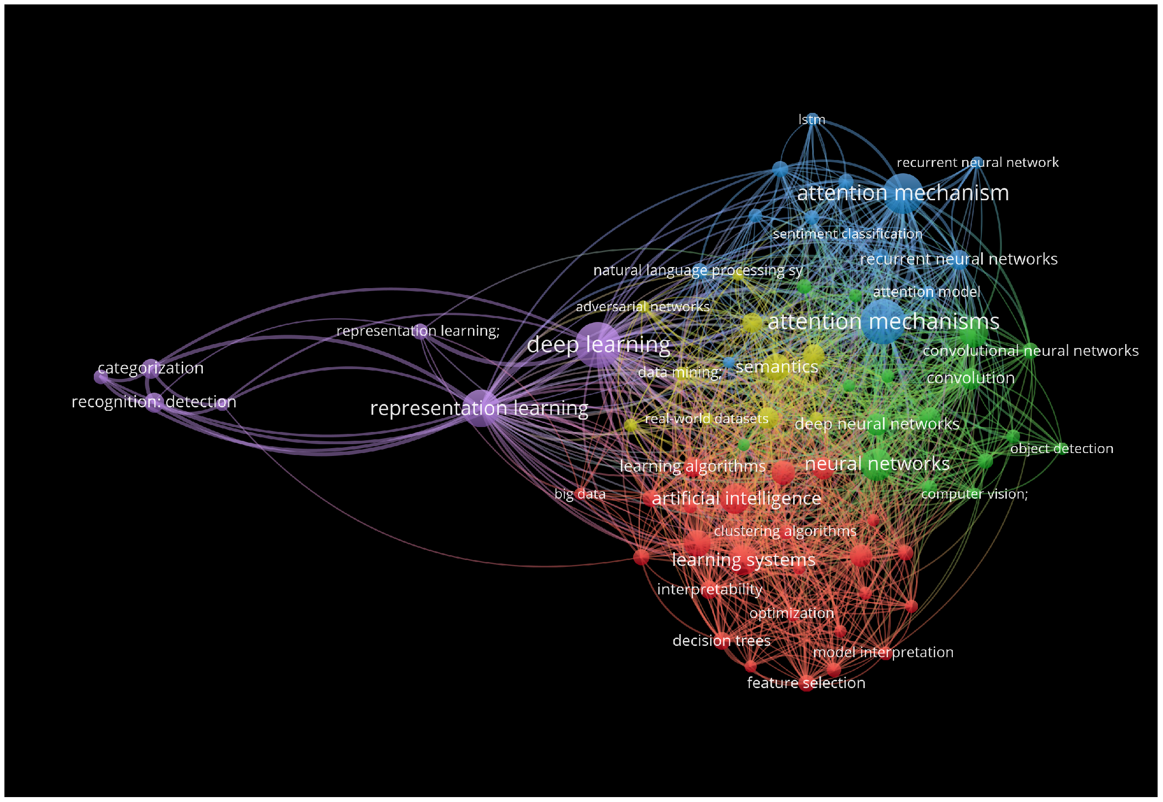
Figure 1. The number of XAI-related articles published over a 20-year Period (January 2002–2021).
Electronics 12 01092 g001
Figure 2. Distribution of XAI-related publications by top 25 learning tasks.
Electronics 12 01092 g002
Figure 3. Distribution of XAI-related publications by subject areas.
Electronics 12 01092 g003
Figure 4. Frequency of explainability synonyms.
Electronics 12 01092 g004
Figure 5. Distribution of algorithms used by researchers in XAI-related publications.
Electronics 12 01092 g005
Figure 6. Co-occurrence network analysis of the keywords used for XAI publications.
Electronics 12 01092 g006
Figure 7. Categorization of Explainable AI research based on current literature. Blue: Self-Explainable Modeling. Black: Model-Agnostic Explainability. Red: Model-Specific Explainability.
Electronics 12 01092 g007
Figure 8. Global intrinsic interpretability methods.
Electronics 12 01092 g008
Figure 9. The encoder–decoder model with a fixed–length context vector of five, translating the sentence “she is eating a green apple” to Chinese. The model could not translate long sentences accurately [51].
Electronics 12 01092 g009
Figure 10. The model by Bahdanau et al. which consists of a bidirectional RNN encoder, an RNN decoder, and an additive shallow feed–forward network for determining attention weights [23].
Electronics 12 01092 g010
Figure 11. Global vs. local attention, the difference lies in using a fixed number instead of all intermediate hidden states [54].
Electronics 12 01092 g011
Figure 12. The x and y-axis correspond to the words in the source sentence (English) and the generated translation (French), respectively. Each pixel shows the weight α i j of the annotation of the j-th source word for the i-th target word, in grayscale (0: black, 1: white) [23].
Electronics 12 01092 g012
Figure 13. Illustration of self-attention mechanism while reading the sentence “The FBI is chasing a criminal on the run”. The color red represents the current word being fixated and blue represents memories. Shading indicates the degree of memory activation [55].
Electronics 12 01092 g013
Figure 14. Global post-hoc interpretability methods.
Electronics 12 01092 g014
Figure 15. ICE and PD Plot, effect of longitude, latitude, housing_median_age, total_room, population, median_income on prediction of Random Forest Regressor for California housing dataset.
Electronics 12 01092 g015
Figure 16. Partial dependence 2D and 3D plot from SKLearn Inspection [61], effect of (AveOccup, HouseAge) on the prediction model (MLP) for California housing dataset.
Electronics 12 01092 g016
Figure 17. Accumulated Local Effects Plot for the previously mentioned variables for the California housing dataset.
Electronics 12 01092 g017
Figure 18. Permutation feature importance boxplot of all features on trained RF model for California housing dataset.
Electronics 12 01092 g018
Figure 19. Global Shapley values ranking using SHAP Bee-swarm and Bar summary plots on our trained RF model for whole datapoints in California Housing dataset.
Electronics 12 01092 g019
Figure 20. SHAP summary plot representing “Course Level Progression” over CGPA value [74].
Electronics 12 01092 g020
Figure 21. Layer-wise Relevance Visualization in a Graph Convolutional Network. Left: Projection of relevance percentages (in brackets) onto the input graph structure (red highlighting). Edge strength is proportional to the relevance percentage an edge carried from one layer to the next. Right: Architecture (replicated at each layer) of the GCN sentence classifier (input bottom, output top). Node and edge relevance were normalized layer-wise. The predicted label of the input was RESULT, as was the true label [95].
Electronics 12 01092 g021
Figure 22. SHAP force plot representing “Course Level Progression” over the CGPA value [74].
Electronics 12 01092 g022
Figure 23. Local post-hoc interpretability methods.
Electronics 12 01092 g023
Figure 24. LIME important features for locality of a random datapoint on the California housing dataset for our trained RF model.
Electronics 12 01092 g024
Figure 25. LIME algorithm for numerical data. (A) Random forest predictions given features ×1 and ×2. Predicted classes: 1 (dark) or 0 (light). (B) Instance of interest (big dot) and data sampled from a normal distribution (small dots). (C) Assign higher weight to points near the instance of interest. (D) Signs of the grid show the classifications of the locally learned model from the weighted samples. The white line marks the decision boundary (P (class = 1) = 0.5) [25].
Electronics 12 01092 g025
Figure 27. LIME explanations for a random datapoint on our trained RF Classifier on BBC news dataset. The words deemed important for predicting the “Tech” class are highlighted, in red (positive influence) and blue (negative influence). In other words, it shows which vocabulary influenced the model to classify this example as a Tech class.
Electronics 12 01092 g027
Figure 28. Beeswarm summary plot and Bar plot based on local Shapley values on the trained Random Forest model for California Housing dataset.
Electronics 12 01092 g028
Figure 29. Left, SHAP explanations for a random datapoint on our trained RF Classifier on BBC news dataset. It demonstrates the most important part of the text (red regions) that increases the output of the RF model and helps the model to classify this example as a tech class. Right, the SHAP summary plot presents a hierarchical group of vocabularies (features) and corresponding Shapley values that increase the output of the RF model.
Electronics 12 01092 g029
Figure 30. The Anchor explanation for the random datapoint on the trained RF model on the California Housing dataset.
Electronics 12 01092 g030
Figure 31. Schematic overview of our proposed black-box adversarial reprogramming (BAR) method [136].
Electronics 12 01092 g031
Figure 32. Example of Diverse Counterfactual Explanation for a random datapoint on a RF model trained on the California Housing dataset.
Electronics 12 01092 g032
Table 1. Different types of attention mechanisms applied in the publications under study.
Attention TypeFrequency
Attention Mechanism221
Self-Attention Mechanism19
Neural Attention Mechanism6
Visual-Attention Mechanism5
Co-Attention Mechanism3
Hierarchical Attention Network2
Inner-Attention Mechanism2
Mutual Attention Mechanism2
Interactive Attention Network1
Compositional Attention Network1
Channel Attention1
Deep Attention Network1
Gated Self-Attention1
Sequence To Sequence Attention1
Simple Neural Attention Meta-Learner1
Intra-Attention Mechanism1
Cross-Attention1
Cross-Layer Attention1
Sequence Generative Adversarial Network1
Table 2. California housing dataset summary of continuous variables.
FeaturesMedian_IncomeHouse_Median_AgeTotal_RoomsTotal_BedroomsPopulationHouseholdLatitudeLongitude
count20,64020,64020,64020,64020,64020,64020,64020,640
mean3.8728.645.431.101425.483.0735.63−119.57
std1.9012.592.470.471132.4610.392.142.00
min0.501.000.850.333.000.6932.54−124.35
25%2.5618.004.441.017872.4333.93−121.80
50%3.5329.005.231.0511662.8234.26−118.49
75%4.7437.006.051.1017253.2837.71−118.01
max15.0052.00141.9134.07356821243.3341.95−114.31
Table 3. XAI use-cases and examples in the AI life-cycle.
Data Collection and Pre-ProcessingModel Building and TrainingEvaluation and Decision-Making
StateBefore training the modelWhile training and refining the modelPost-training, after the AI system and model is built- this process can be iterative depending on the feedback from the client(s).
PurposeReading into the data, and pre-processing for further analysesGenerating ML model(s) and AI system(s) to meet the clients’ requirementInsight generation, decision-making, and planning intervention
Tasks InvolvedSetting up a data collection protocol and pipeline, data cleaning, formatting, feature engineering (feature selection, calculating mostly correlated features and variance, etc.)Development of machine learning models by tuning hyper-parameters to fit the data and problem, database setup, and AI GUI/system development for presenting results and communicating with clientsGenerating reports based on evaluation metrics, visualization, and conducting user studies with clients and domain experts for feedback, etc.
Primary Stakeholders InvolvedPrimarily all stakeholders involved in the AI life cycle—clients, domain experts, software developers, and data scientists: It establishes a communication channel between the vendor(s) and the client(s) for defining the requirements.Software developers and data scientists: This stage requires medium to advanced data science knowledge to develop machine learning models. If the objective is to build a system or tool, data scientists may collaborate with software developers or make it themselves if they have prior experience in software development.Primarily all the stakeholders are involved through agile methodology-incremental feedback and fine-tuning models and systems until the final product is ready.
Use-case(s)Bridging the Gap Between Data Scientists and Non-data Science ExpertsFine-tuning, model comparisons to find the best model, Debugging and AssuranceHuman-assisted AI for decision-making in different domains, Fine-tuning and Training AI Models, Bridging the Gap Between Data Scientists and Non-data Science Experts, Trust, Accountability, and Fairness
Example XAI tools and TechniquesDifferent visualization plots such as pair correlation, Individual Conditional, Partial Dependence, Accumulated Local Effect plots, etc.Some categories of Intrinsic, Ad-hoc and global and local post-hoc model-specific and model-agnostic explanations such as DL representation explanations, global and local attention models, joint prediction and explanations, perturbation-based explanations, kernel SHAP, layer-wise relevance propagation, adversarial over transformations, etc.Some categories of global and local model-specific and model-agnostic explanations such as Global Shapely values, feature weights in GAM, Anchor and LIME; feature importance-based and saliency visualization-based explanations, etc.
Disclaimer/Publisher’s Note: The statements, opinions and data contained in all publications are solely those of the individual author(s) and contributor(s) and not of MDPI and/or the editor(s). MDPI and/or the editor(s) disclaim responsibility for any injury to people or property resulting from any ideas, methods, instructions or products referred to in the content.

