Detecting and Localizing Anomalies in Container Clusters Using Markov Models


Software and Systems Engineering Group, Free University of Bozen-Bolzano, 39100 Bolzano, Italy
*
Author to whom correspondence should be addressed.
Electronics 2020, 9(1), 64; https://0-doi-org.brum.beds.ac.uk/10.3390/electronics9010064
Submission received: 6 November 2019
/
Revised: 3 December 2019
/
Accepted: 12 December 2019
/
Published: 1 January 2020
(This article belongs to the Section Computer Science & Engineering)
Abstract
:Detecting the location of performance anomalies in complex distributed systems is critical to ensuring the effective operation of a system, in particular, if short-lived container deployments are considered, adding challenges to anomaly detection and localization. In this paper, we present a framework for monitoring, detecting and localizing performance anomalies for container-based clusters using the hierarchical hidden Markov model (HHMM). The model aims at detecting and localizing the root cause of anomalies at runtime in order to maximize the system availability and performance. The model detects response time variations in containers and their hosting cluster nodes based on their resource utilization and tracks the root causes of variations. To evaluate the proposed framework, experiments were conducted for container orchestration, with different performance metrics being used. The results show that HHMMs are able to accurately detect and localize performance anomalies in a timely fashion.
1. Introduction
Many distributed software systems, such as clouds, allow applications to be deployed and managed through third-party organizations in order to provide shared, dynamically managed resources and services [1]. Understanding the behaviour of such systems is difficult as it often requires to observe larger numbers of components such as nodes and containers over longer periods of time. Due to the distributed nature, heterogeneity, and scale of many container deployments, performance anomalies may be experienced leading to system performance degradation and potential application failures. A performance anomaly arises when a resource behaviour (e.g., CPU utilization, memory usage) deviates from its expectation. Such a performance anomaly is difficult to detect because normal performance behaviours are not always established. An unsolved aspect for resource management for containers is that applications running in containers are not aware of their resource limits. Thus, if an application attempts to automatically configure itself by allocating resources based on the total node resources available, it may over-allocate when running in a resource-constrained container.
In particular, with the recent attention that microservice architectures have received [2,3], their dynamic management is of particular importance [4,5].
There are many studies regarding detecting anomalies in cloud and edge computing contexts [6,7], and specifically in containerized environments [8,9,10]. Some studies looked at detecting an anomaly’s root cause in clouds at a virtual machine [7,11] or network level [12]. Detecting and localizing anomalies in clustered container deployments [13] is still recognized as a research gap [8,14].
We develop a mechanism that identifies the symptoms of an anomaly if its performance differs from the expected behaviour. We identify anomalous performance once it generates unpredictable time-varying workload, which puts strains on different resources (e.g., CPU or memory) at different times. In order to detect anomalous behaviour and to find its root cause in such an environment, there are two main challenges: (1) What metrics should be monitored? (2) How to accurately detect and identify the anomalous behaviour in a container-based cluster? Metrics are collected from the monitored resources of the system components at different abstraction levels [15]: (1) Resource Utilization as the proportion of the resources in use (CPU, Memory) to the total number of resources provided per time unit; (2) Response Time as the time taken by a request until the arrival of the response; (3) Throughput as the average number of requests per second processed by one instance.
In order to understand an observed performance degradation, we introduce a framework for detecting and localizing performance anomalies in container clusters. A performance anomaly indicates a deviation from its normal behaviour in a component’s workload. To detect an anomaly and to localize its root cause, we use a hierarchical hidden Markov model (HHMM) [16], which is a doubly stochastic process model used for modeling hierarchical structures of data at multiple length/time scales. The framework consists of two phases. Detection detects workload behaviour of components based on their observed response time and resource utilization. Identification identifies the cause of a detected anomalous behaviour on multiple paths, where a path is defined as a link between two components (e.g., container and node). Once an anomaly is detected, identification follows. In both phases HHMMs are applied to detect anomalous behaviour, localize the root cause that is responsible for the observed anomaly, and determine the dispersal of the anomaly within the system.
The evaluation of the proposed framework is based on analyzing datasets extracted from multiple container systems. Our experiments show that once HHMM is configured properly, they can detect anomalous behaviour and identify its root-cause with more than 94.3% accuracy.
2. Related Work
This section presents a review of the models for detecting and localizing anomalies in distributed environments in general and specific using the HHMM.
Du et al. [8] use different machine learning techniques to detect anomalous behaviour for microservices with container deployment. Dullmann [10] provides an online performance anomaly detection approach that detects anomalies in performance data based on discrete time series analysis. Sorkunlu et al. [17] identify system performance anomalies through analyzing the correlations in the resource usage data. Wang et al. [9] model the correlation between workload and resource utilization of applications to characterize the system status. Alcaraz et al. [7] detect anomalous behaviour in virtual networks using the Random Forest algorithm. The authors evaluate their approach by injecting anomalies and generating workload that affect the CPU and memory. In [18], the authors detect anomalous behaviour in cloud applications using the Principal Component Analysis (PCA). In [19], the authors use crosscutting concern (Aspect-Oriented Programming AOP), to detect anomalies in web applications under different workloads based on measuring CPU, memory, network and disk. Kozhirbayev et al. [20] study the performance of container platforms running on top of IaaS. The authors compare the performance of the Docker, the Flockport (LXC) with their VM environment in different types of workloads. They made a comparison to explore the performance of CPU, memory and disk with different benchmarks. The results are based on the metrics measured by the benchmarking tools.
Peiris et al. [21] analyze the root causes of performance anomalies of CPU usage by combining the correlation and comparative analysis techniques in distributed environments. The work in [11] analyzes workload to detect performance anomalies and categorizes performance anomalies into three layers: (1) symptoms, externally visible indicators of a performance problem, (2) manifestation, internal performance indicators or evidences, and (3) root causes, physical factors whose removal eliminates the manifestations and symptoms of a performance incident.
Moreover, HMMs and its derivations are used to detect anomalies. In [22], HMM techniques are used for the detection of anomalies and intrusions in a network. In [23], the author detects faults in real-time embedded systems using a HMM through describing the healthy and faulty states of a system’s hardware components. In [24], a HMM is used to find which anomaly is part of the same anomaly injection scenario. In [25,26], we define a HMM-compliant controller architecture for basic anomaly detection and also address self-healing, but in this paper we give more details about the work for container-oriented detection and identification using HHMM to be able to trace the anomaly behaviour.
To move beyond these works, our framework focuses on detecting and identifying anomalous behaviour in container clusters. We use the response time and resource utilization (CPU and memory) measurements of components to construct an HHMM. The HHMM observes the response time variation of nodes and containers and relates it to the workload, which is hidden from the observer. We adopt the HHMM to study behaviour in such environments and to reflect the structure of our system. This extends earlier work [27] towards identification and root cause analysis that here builds on the more generic Hierarchical Hidden Markov Models (HHMM) as the formal model compared to the earlier HMMs used, thus allowing better root cause analysis in layered (hierarchical) architectures.
3. Hierarchical Hidden Markov Model (HHMM) for Anomaly Detection in Container Clusters
HHMMs are a generalization of the hidden Markov model approach (HMM) that is designed to model domains with hierarchical structure [16].
3.1. HHMM Basic Structure and Definition
The HMM emit symbols in the process states they are in. HHMMs do not emit observable symbols directly as they are constructed by one root state composed of a sequence of substates [16]. Each substate may consist of another substates and generates sequences by recursive activation. The process of recursive activations stops when it reaches a production state. The production state is the only state that emits output symbols like a HMM. The other states that emit substates instead of output symbols are called internal states or abstract states. The process that an internal state activates a substate is termed a vertical transition, while a state transition at the same level is called a horizontal transition. When a vertical transition is completed, the state which started the recursive action will get the control and then perform a horizontal transition.
A HHMM is identified by , where is a set of parameters consisting of state transition probability A; observation probability distribution B; the state space at each level, and the hierarchical parent-child relationship , ; consists of all possible observations O. consists of horizontal and vertical transitions between states (d specifies the number of hierarchical levels). is the initial transition for the states . Importantly, the states in the HHMM are hidden from the observer and only the observation space is visible.
There are three problems that the HHMM needs to address [16]:
- Calculating the likelihood of a sequence of observations: given a HHMM and its parameter set, find the probability of a sequence of observations to be generated by the model. The first problem can be used to determine which of the trained model is most likely when a training observation sequence is given. In our performance analysis case of containerized-cluster environment, given the previous observations of the containers, the model detects the anomalous behaviour. To achieve this step, the model is designed to adjust and optimize its parameters.
- Finding the most probable state sequence: given the HHMM, its parameter set, and an observation sequence, find the state sequence that is most likely to generate the observation (finding out the hidden path of anomalous observation). In our case, we apply the model to track the sequence of anomalous behaviour in the system. At this problem, number of different observations should be applied to the model to refine its parameters. At this stage, we use the Viterbi algorithm.
- Estimating the parameters of a model: given the structure of the HHMM and its observation sequences, find the most probable parameter set of the model. The third problem deals with the model training. In our case, once the model has been thoroughly optimized, we train the model with historical and runtime data to perform detection and tracking enhancement. The Baum-Welch algorithm is used to train the model.
To achieve that, the model must be able to: (1) efficiently analyze large amounts of data to detect potential anomalous observation in a containerized-cluster environment; (2) identify the root-cause of the captured anomaly; and (3) report the identified anomaly along with its path.
3.2. Customizing HHMM for Anomaly Detection in Container Clusters
In our case, the system in question is hierarchical, composed of nodes. A node consists of one or more containers. Each container has an application that runs on it. Containers may communicate within the same node or externally. Thus, we apply the HHMM to describe the behaviours of such hierarchical systems. Our HHMM is composed of:
- Cluster: which is the root state in the model. It is responsible for controlling nodes and containers, which are the states. A cluster consists of at least two nodes and multiple containers.
- Nodes, i.e., resources that offer capacity to its containers such as Memory and CPU. The main job of the node is to perform requests to its underlying substates, which are the containers in our case. The system may contain one or multiple nodes belongs to one cluster. In our HHMM, nodes are substates, and they may be internal states, if they do not emit any observation. In case a node emits an observation, it is considered a production state. In such situation, a production state cannot have substates as it is considered a leaf in the hierarchy.
- Containers, i.e., lightweight virtualized execution units that can run an application in an isolated environment. One or multiple containers can run on the same node and share its resources. As specified in the node, a container is considered an internal state if it does not emit any observation. Otherwise, it is considered a production state.
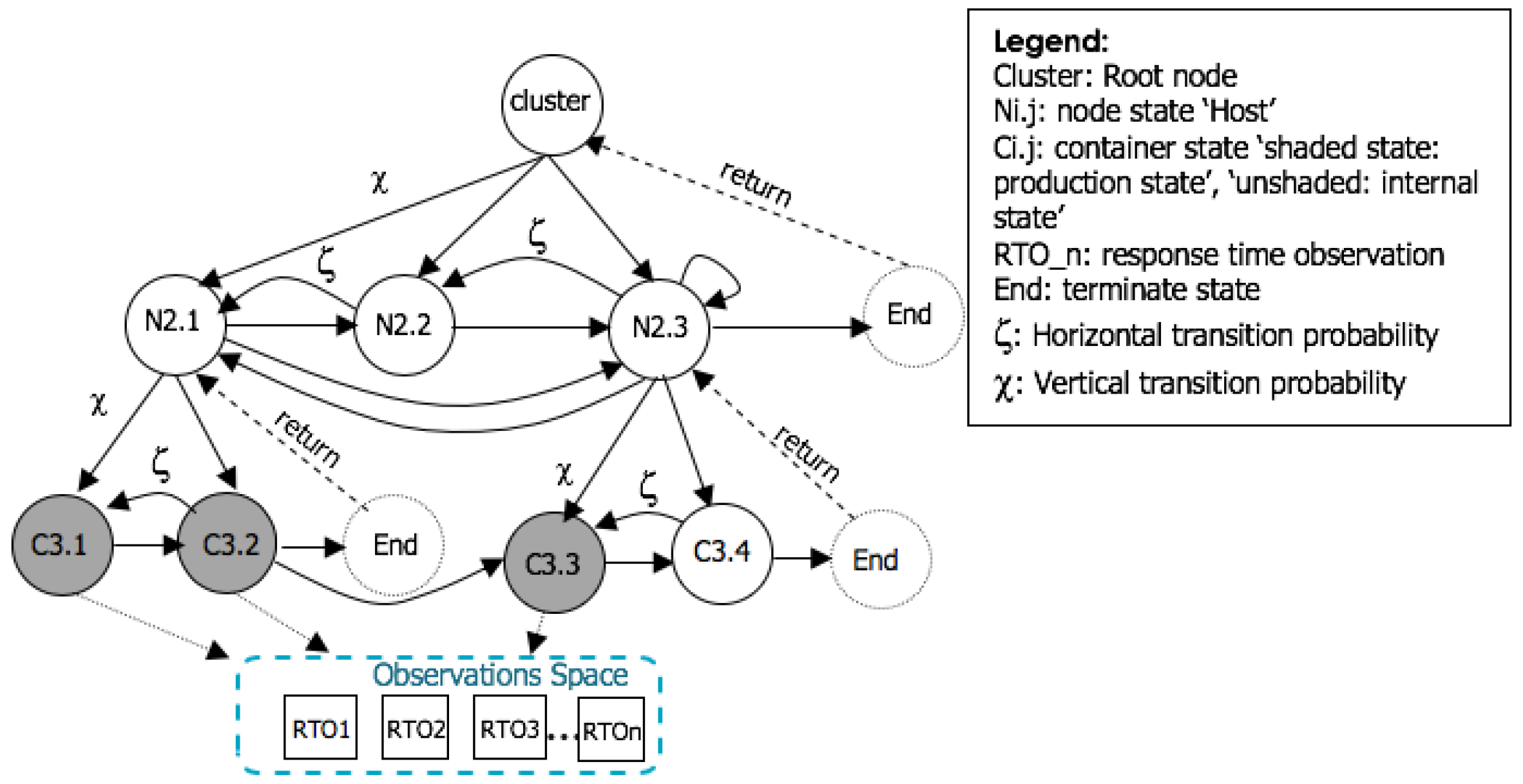
To meaningfully represent our system topology, we modify the HHMM annotations. As shown in Figure 1, the q state is mapped to with hierarchy index j = 1, the internal state that emits substates is mapped to to represent nodes, and the production state is mapped to to represent containers that emit observations. The i is the state index (horizontal level index), and j is the hierarchy index (vertical level index). The observations O are associated to the response time fluctuation that are emitted from containers or nodes. The node space contains set of nodes and containers, e.g., , , .
The HHMM vertically calls one of its substates such as or with vertical transition . Since is an abstract state, it enters its child HMM substates and . Since is a production state, it emits observations, and may make a horizontal transition from to . Once there is no another transition, transits to the state, which ends the transition for this substate, to return the control to the calling state . Once the control returns to the state , it makes a horizontal transition (if possible) to state , which horizontally transits to state . State has substates that transits to , which may transit back to or may transit to the state. Once all transitions under this node end, then the control returns to . State may loop around, transit back to , or enter its end state, which ends the whole process and returns control to the cluster. The model can not horizontally transit unless it vertically transited. Furthermore, the internal states do not need to have the same number of substates. It can be seen that calls containers and , while has no substates. The edge direction indicates the dependency between states. This type of hierarchical presentation easily aids in tracing the anomaly to a root cause.
Each state may have workload associated to CPU or memory utilization. Such workload can be detected through observing the fluctuations in response time, which is emitted by the production states ’container’ or some of the ’nodes’. Workload in a state not only affects the current state, but it may affect other levels. However, container workload only affects the container itself. The horizontal transition between containers reflects the request/reply between the client/server in our system under test, and the vertical transition refers to the child/parent relationship between containers/nodes.
The HHMM is trained on response time over the hidden CPUs and memory resources assigned to the components. A trained probabilistic model can be compared against the observed sequences to detect anomalous behaviour. If the observed sequence and predicted sequence are similar, we can conclude that we have a model learned on normal behaviour. In that case, the approach will declare the status of the system ’Anomaly Free’ (no observed anomaly). Learning the model on normal behaviour aids in estimating the probability of each observed sequence, given the previously observed sequence. We call the sequence with the lowest estimated probabilities anomalous. In case of an anomaly, the model traces to the root cause of anomaly and determines its type. At the end, the path of the identified anomaly and the anomaly type is produced. The trained HHMMs are stored in the “Basic Configuration” file to be used in the future. The model is trained on observations until parameter convergence (A, B, , , become fixed). Since the HHMM parameters are trained during runtime on continuously updated response times of components, we use the sliding window technique [28] to read the observations with window size = 10–100 observations, which generates multiple windows with different observations. The obtained observations are used to feed the HHMM.
4. An Anomaly Detection and Identification Framework
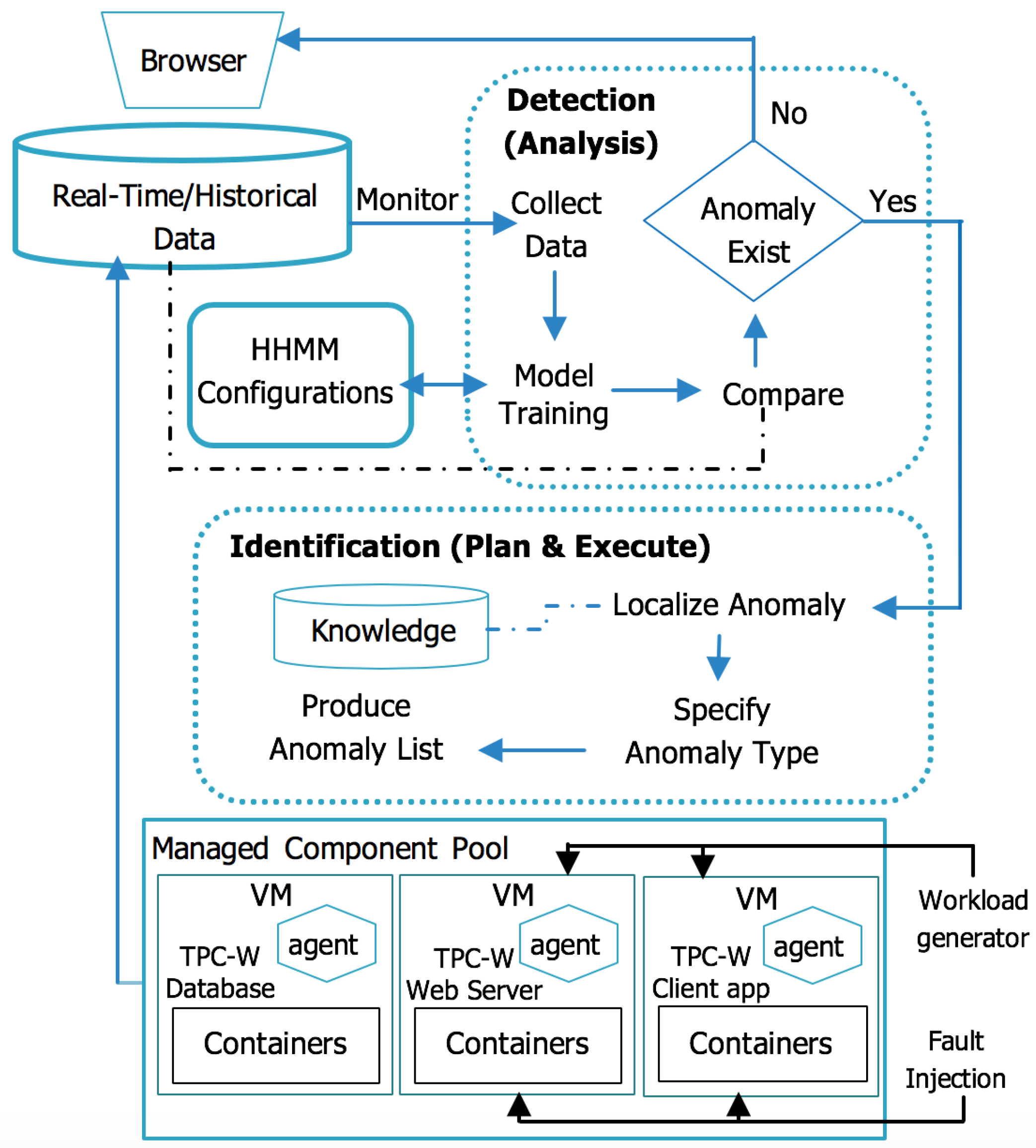
Our anomaly management framework consists of two main phases: detection and identification [25]. The detection phase detects the existence of anomalies in system components. The identification phase is responsible for processing the output of the detection phase in order to track the cause of an anomaly and identify the anomaly type through observing variations in the response time of components. Each phase is accompanied by the Monitor, Analysis, Plan, and Execute-Knowledge (MAPE-K) control loop:
- Monitor: collects data about components and resources for later analysis. Data is gathered from an agent that is installed on each node. We use the spearman rank correlation to capture the existence of anomalous behaviour.
- Analysis: once data is collected, we built HHMMs for the system as shown in Figure 1 to provide a high level of performance over the entire detection space. At this stage, a HHMM detects the existence of anomalous behaviour.
- Plan and Execute: when the HHMM detects an anomaly, it tracks its path and identifies its type.
- Knowledge: a repository with different anomaly cases that occur at different levels. Such cases are used by the plan and execute stage to aid in identifying the type of the detected anomaly.
4.1. Anomaly Cases
Because of the transient nature and growing scale of containers, it is often difficult to track the workload of individual containers. Thus, we also analyze the variation of response time for container and node performance. We define different types of anomaly based on observing our system behaviour (Figure 1) and exploring the common anomaly cases that are reported [6,29,30,31]. The following lists different anomaly cases focusing on workload and response time [25,26]:
Case 1: Low Response Time Observed at Container Level
- Case 1.1 Container Overload (Self-Dependency): a container enters into a self-load loop because it is heavily loaded with requests or has limited resources. This load results in low container response time. This case may apply for one or multiple containers with no communication.
- Case 1.2 Container Sibling Overload (Inter-Container Dependency): an overloaded container may indirectly affect other dependent containers at the same node. For example, has an application that almost consumes its whole resources. When it communicates with and is overloaded, then will go into underload because and share resources of the same node.
- Case 1.3 Container Neighbour Overload (External Container Dependency): happens if one or more communicating containers at different nodes are overloaded. For example, shows low response time once is overloaded as depends on , and depends on to complete user requests. Thus, a longer response time occurs for those containers.
Case 2: Low Response Time Observed at Node Level
- Case 2.1 Node Overload (Self-dependency): node overload happens when a node has low capacity, many jobs waiting to be processed, or network problems occur. For example, has limited capacity, which causes an overload at container level for and .
- Case 2.2 Node Overload (Inter-Node Dependency):an overloaded node may indirectly affect other nodes in the same cluster. This may cause low response time observed at node level, which slows the whole operation of a cluster because of the communication between the two nodes assuming that and share the resource of the same cluster ’physical server’. Thus, when shows a heavier load, it would affect the performance of .
There are different anomalies that may lead to these different cases, such as infrastructure issues (e.g., service down), hardware issues (e.g., CPU, memory or disk down), kernel issues (e.g., kernel deadlock, corrupted file system), container runtime issues (e.g., unresponsive runtime), file configuration issues, or change in cluster management tool versions. We can observe from these cases that there are two types of anomaly propagation, at node level (), which happens due to the collocation relationship between different nodes, and at container level, which occurs due to application calls at different nodes ().
To simplify the anomaly identification, we focus on hardware and runtime issues and we assume that not all nodes will go down at the same time. We assume to have prior knowledge regarding: (1) the dependency between containers and nodes; (2) response time, memory utilization and CPU utilization for containers and nodes.
4.2. Anomaly Detection and Identification Mechanism
4.2.1. Anomaly Monitoring
In order to detect anomalous behaviour, data is collected from the “Managed Component Pool”. Each node in the pool has an installed agent that is responsible for exposing log files of containers and nodes to the Real-Time/Historical Data storage component. The metrics include information about the resources of components at container/node level such as CPU utilization, memory usage, response time, number of available running container, number of nodes, and container application throughput. The aim from collecting data is capturing the system status to study its resource consumption to be able to assess the overall performance of the system.
Before building the HHMM, we check if there is a performance variation at container/node level and we verify if it is a symptom of an anomaly. Thus, we use the Spearman’s rank correlation coefficient to estimate the dissociation between different numbers of user requests and the collected parameters from the monitored metrics. If there is a decrease in the correlation degree, then the metric is not associated with the increasing number of requests, which means that the observed variation in performance is not an anomaly, but may relate to system maintenance. In case the correlation degree increases, this refers to the existence of anomalies occurring as the impact of dissociation between the number of user requests and the monitored metric exceeding a certain value. Algorithm 1 defines a threshold to signal an anomaly occurrence. The degree of dissociation (DD = 60 for CPU utilization; DD = 20 for memory utilization) can be used as an indicator for performance degradation.
| Algorithm 1 Check Performance Degradation |
1: Initialization:
array to store interval in minutes 3: Begin 4: ; 5: ; 6: while do 7: ; 8: ; 9: end while 10: ; 11: ; 12: End 13: Output: return |
Line 1 initializes the parameters. Line 2 defines the interval as a time window in which the user requests occur. Lines 4–9 loop to retrieve user requests (line 4) from the repository for all containers that run the same application in a specific interval. The monitored metrics for the same containers and their nodes are retrieved for the user requests (line 7). Line 10 calculates the spearman correlation for the user requests and the measured metric as shown in Equation (1). The URi refers to the ranks of the UR, and the UR is the mean ranks of the number of user requests processed in an interval. The Mi refers to the ranks of the monitored metric values (i.e., the sequence of the accumulated response time per user transaction). M is the mean rank. The result of SC can be interpreted as in [32]: [0.70, 1.0] which stands for a strong correlation, [0.40, 0.69] which stands for a medium correlation, between [0.0, 0.39] there is no correlation. Line 11 calculates the variance by measuring the difference between the current interval and the highest old one for both the monitored metric and the user requests. The product for the estimated variance to obtain one threshold is calculated. Equation (2) shows the which is the average of the monitored metric (e.g., response time). The is the previous value of the monitored metric in a given interval. The is the new value of the monitored metric in a given interval. The is the previous value of the user requests (e.g., user interaction) in a given interval. The is the new value of the user requests in a given interval. n is the number of periods in a given interval (e.g., an interval is made up of 10 periods, each period is 5 min). The is the maximum value of the , which is calculated through subtracting the observed in a current interval from the maximum value of the previous interval as shown in (3). Line 12 returns the threshold (DD) as an indicator for anomaly occurrence for the chosen metric as shown in (4).
4.2.2. Anomaly Detection and Identification: Analysis and Execute
An algorithm to detect and identify anomalous behaviour is shown in Algorithm 2. Line 1 initializes the parameters. Line 2 represents the inputs for the algorithm. Lines 4–18 represent the initialization and training of the HHMM using the Generalized Baum-Welch algorithm [16] to train the HHMM by calculating the probabilities of the model parameters. The output of Baum-Welch is used in the identification step. In lines 19–21, the Viterbi algorithm is used to find the path of the detected anomalous states. At this step, we obtained the states, probabilities, and state sequence. Once we obtain the anomalous states, we list the states chronologically to locate the state that shows the first presence of the anomaly. For each state, we know the time of its activation, its last activated substate, and the time at which the control returned to the calling state. By the end of that step, we obtain a matrix that contains the anomalous states, their scope, probability and transitions. Lines 22–41 iterate over the result in order to check the anomaly case. The algorithm finishes by returning the anomaly case and the path of the anomalous state.
| Algorithm 2 Detection-Identification Algorithm | |
1: Initialization:
4: Initialize HHMM: 5: if then 6: initialize HHMM parameters; 7: else 8: initialize HHMM parameters with the last updated values; 9: end if 10: Training HHMM 11: Detection 12: do | |
| 13: ; | ▹ run Baum-Welch algorithm |
| 14: ; | ▹ update all Baum-Welch parameters |
| 15: ; | ▹ sotre updated values in , , |
| 16: ; | ▹ increase the model iteration number |
| 17: while 18: ; 19: Identification 20: ; 21: ; 22: for each r in do 23: for each c in do 24: if ( AND AND ) then 25: case ← Container Sibling Overloaded (Inter Container Dependency); 26: else if ( AND AND ) then 27: case ← Container Overloaded (Self-Dependency); 28: else if ( AND AND ) then 29: case ← Container Neighbor Overloaded (External Container Dependency); 30: else if ( AND AND ) then 31: case ← Inter Node Dependency; 32: else 33: case ← Node Overload (Self-dependency); 34: end if | |
| 35: ; | ▹ increment c |
| 36: end for 37: ; | |
| 38: ; | ▹ increment r |
| 39: end for 40: End 41: Output: case, path | |
5. Evaluation
We can monitor, detect and localize anomalous workload in nodes and containers by considering different performance measurements such as CPU, memory, and throughput metrics. Thus, to assess the effectiveness of our solution, we investigate different anomaly scenarios using the TPC-W (http://www.tpc.org/tpcw/), an industry-standard benchmark, and apply the HHMM to detect and identify the injected anomalies. In this section, we first introduce the experimental setup and the chosen benchmark in Section 5.1. Then, in Section 5.2, we explain the anomaly injection and workload settings developed and selected for the experiments. In Section 5.3, we apply the framework to detect and identify anomalies. Section 5.4 compares our framework with other common anomaly management solutions. In order to avoid threats to the validity of the work, we also consider the effect of other monitoring tools as critical components on the results in Section 5.5.
5.1. Experimental Set-Up
The TPC-W benchmark is used for resource provisioning, scalability and capacity planning for e-commerce websites. The TPC-W emulates an online bookstore that consists of 3 tiers: client application, web server, and database. The experiment platform is composed of several VMs. Each tier is installed on a VM. We do not consider the database tier in the anomaly detection and identification as a powerful VM should be dedicated to the database. The web server is emulated using a client application which simulates a number of user requests that is increased iteratively. The experiment environment consists of 3 nodes , , , each equipped with containers. As shown in Figure 2, is the TPC-W client application, holds the TPC-W database, and the TPC-W server.
Each VM is equipped with Linux OS (Ubuntu 18.04.3 LTS x64), 3 VCPU, 2 GB VRAM, Xen 4.11 (https://xenproject.org/). The virtual experiment is run on a PC equipped with Intel i5 2.7GHz, Ubuntu 18.04.3 LTS x64, 8 GB RAM and 1 TB storage. The VMs are connected through a 100 Mbps network. The SignalFX Smart Agent (https://www.signalfx.com/) monitoring tool is used to observe the runtime performance of components and their resources. The agent is deployed on each VM to collect and store performance metrics of the system under test. The experiments focus on CPU and memory utilization metrics, which are gathered from the web server. The Response time is measured at the client’s end. We further use docker command to obtain a live data stream for running containers, to know the CPU utilization rate, and to collect information about memory usage. Table 1 shows the monitoring metrics collected.
There are 1511 records in the generated datasets: 650 records in dataset ‘A’ from VM1 and 861 records in dataset ‘B’ from VM3. For each of the datasets, 50% of the records are used as a training set to train the model, and the rest are used as a test set to validate the model. The TPC-W benchmark is running on containers. The number of the replica of containers is set to two. The performance data of the benchmark is gathered from all the containers that ran this benchmark and their hosting nodes. The collected data is used to train the HHMM model to detect and identify the anomalies in containers and nodes. The experiment is repeated 10 times, and the model training lasts 150 min for all the experiments with results varying according to the number of states. Table 2 and Table 3 show the physical system properties and the virtualized environment settings under observation.
To obtain historical data, the TPC-W is run for 300 min. The data used for simulation is created by a workload generator active at different times. The workload of each container is similar. The workload is generated by the TPC-W client application. The TPC-W contains its own workload generator (RBE) that emulates the behaviour of end-users, and reports metrics such as the response time and throughput of the server. We create a workload that runs for 49 min. Since the workload is always described by the access behaviour, the container is gradually loaded with [30–100,000] emulated user requests. The number of emulated user requests is changed periodically.
We use the Heapster (https://github.com/kubernetes-retired/heapster) to group the collected data and store them in the time series database the InfluxDB (https://www.influxdata.com/). The gathered data from the monitoring tool and from datasets are stored in “Real-Time/Historical Data” storage to allow for the future anomaly detection and identification. We use Grafana (https://grafana.com/grafana/testimonials/) and the Datadog (https://www.datadoghq.com/) to support online data gathering. As output format for the collected data, we use CSV files to read and write data that is used to feed offline experimental data.
5.2. Anomaly Injection and Workload Contention Scenarios
To create pressure on the system and generate different workloads, the following shows the anomaly injection approach and the workloads that are applied at different system levels.
5.2.1. Resource Exhaustion
For simulating realistic anomalies in the system, a script is written to inject different types of anomalies into the target system, shown in Algorithms 3 and 4. The anomalies types (CPU Hog and Memory Leak) are taken from real-world scenarios [8,9,33].
| Algorithm 3 Anomaly Injection Algorithm at Container Level |
1: Input:
3: for each do 4: for each do 5: for each do 6: InjectAnomaly(, , ); 7: ; 8: end for 9: end for 10: end for 11: End 12: Output: , at |
| Algorithm 4 Anomaly Injection Algorithm at Node Level |
1: Input:
3: for each do 4: for each do 5: InjectAnomaly(, , ); 6: ; 7: end for 8: end for 9: End 10: Output: , at , |
CPU Hog: A CPU hog can be due to an unplanned increase in user requests. It causes anomalous behaviour in a component, e.g., component not responding fast enough or hanging under heavy load. The CPU injection happens at different containers levels and at node level . We do not consider as it is representing the database.
Memory Leak: Here, the usage of memory available in the component is increased over a relatively short period of time. If all the memory is consumed, then the framework will declare the status of a component as anomalous. The memory injection happens at .
5.2.2. Workload Contention
Workload contention occurs when an application imposes heavy workload on system resources, which results in performance degradation. Workload contention might occur due to limited resources or increasing the number of requests. In this experiment, the workload contention is applied at container level. Table 4 shows the configuration parameters that are used to create different workload contentions. Table 5 summarizes the types of anomaly injections and workload generation.
5.3. Detection and Identification of Anomaly Scenarios
Training a model to detect and identify anomalies requires training data. However, the availability of such data is limited due to the rarity of anomaly occurrences and the complex manual training process. Consequently, extreme resource contention situations are generated, and different types of anomalies are injected to work with more realistic scenarios for the experiments, and to collect performance data for different system conditions to assess the anomaly detection and identification.
The anomalies are simulated using the stress (https://linux.die.net/man/1/stress) tool, which is used to conduct pressure tests. In each experiment, one type of anomaly is injected. The anomaly injection varies slightly depending on the anomaly type. The anomaly injection for each component lasts 2 min. For each anomaly, the experiment is repeated 10 times. The injection period is changed from one experiment to another. After the injection, datasets with various types of anomalies from different containers and nodes are created. Such datasets are used to assess the anomaly detection and identification performance of the proposed framework. Once the datasets are generated, the HHMM model is retrained on anomalous data. The result of the model is used for the validation.
To address the anomaly cases from Section 4, the injection is done in two steps: at system level and for each component at a time. Thus, the injection start and end times differ from one component to another. The following discusses detection and identification of injected anomalies at different levels.
5.3.1. System-Level Injection
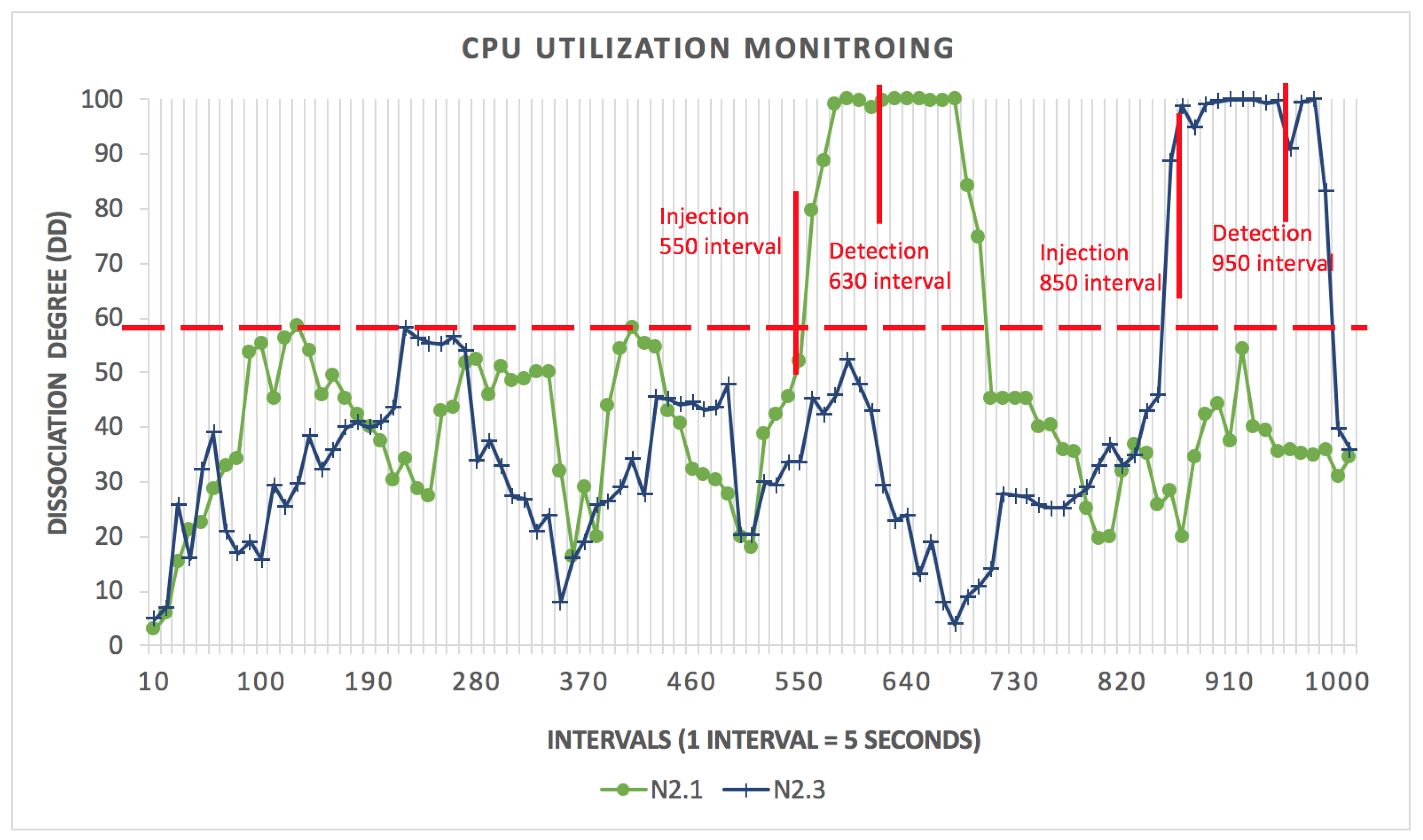
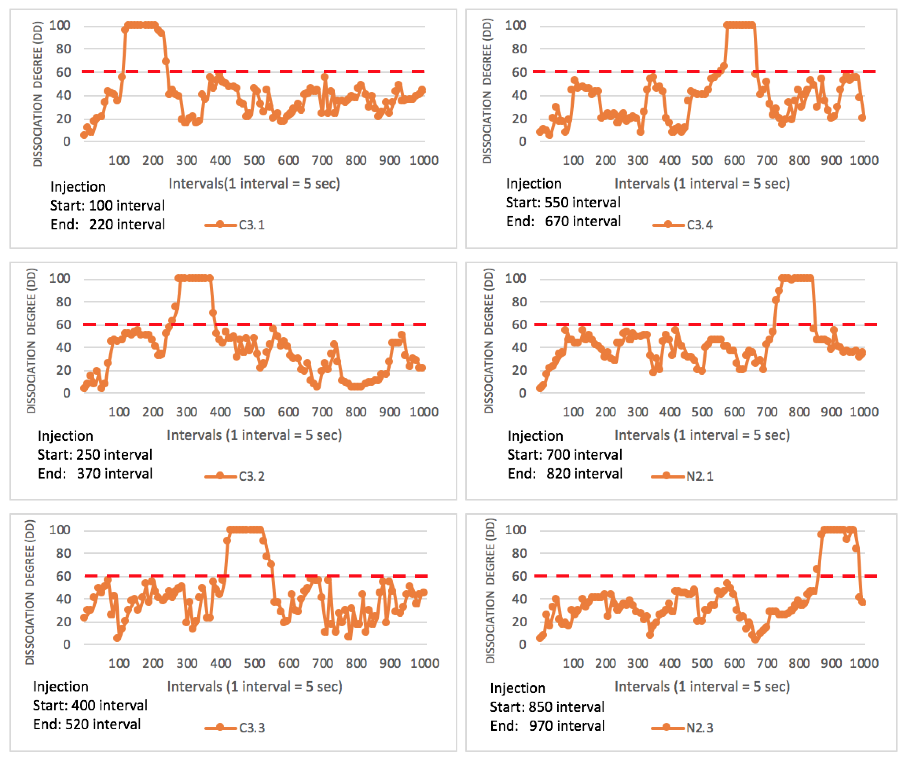
The anomaly is injected at and . For the CPU hog, the injection begins at time interval 550 (1 interval = 5 s) for and interval 850 for . The dissociation degree shows an anomaly as the CPU performance exceeds the threshold (DD = 60). After training the HHMM, the model detects the anomalous behaviour for at the 630 interval time, and for at 950 as shown in Figure 3.
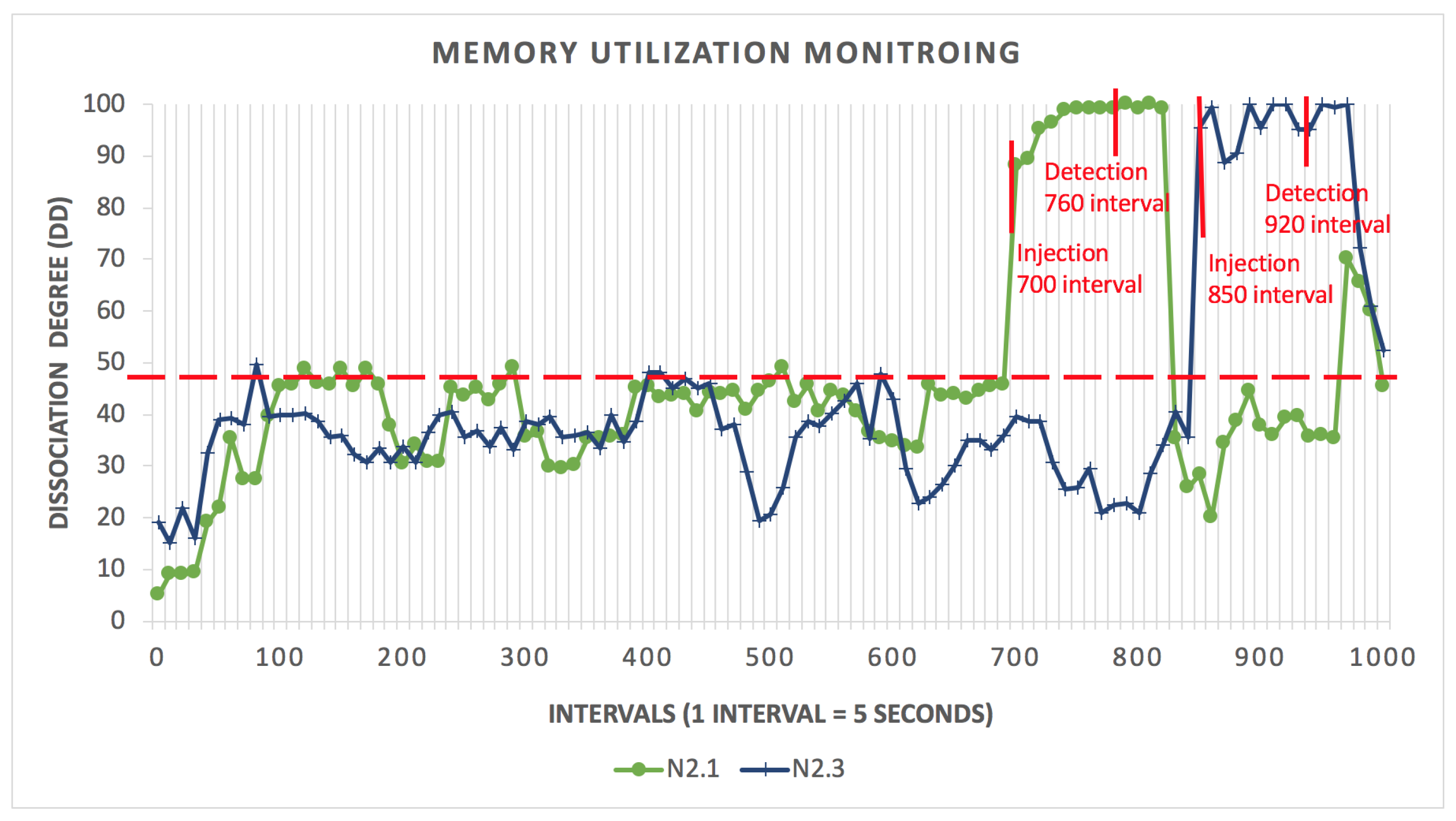
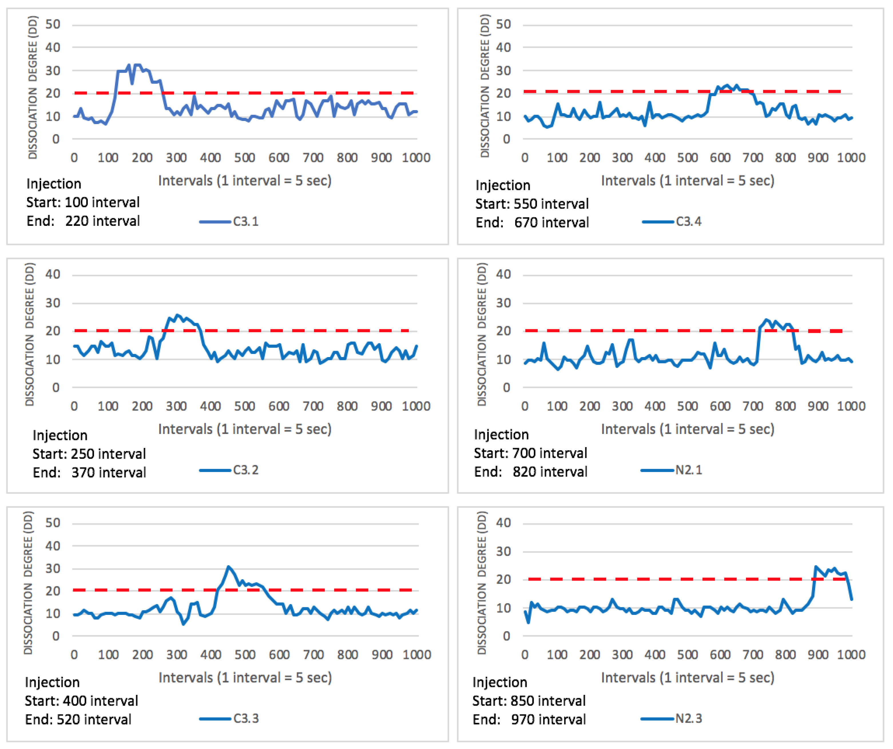
The same situation applies for the memory leak. The injection begins at intervals 700 and 850 for and , respectively. As depicted in Figure 4, the model detects the anomalous behaviour for and at intervals 760 and 920.
The injection of anomalies at node level affects container that are connected to the anomalous node. To identify the anomalous path, and to return the anomaly type, the model determines paths of anomalous behaviour and returns the paths of the most likely anomalous sequence ordered chronologically based on which one showed anomalous behaviour first. Once we obtain the path, the algorithm checks the anomaly cases and selects the matching one as shown in Algorithm 2.
5.3.2. Component-Level Injection
The anomalies were injected for each component in the system. Figure 5 and Figure 6 show the injection period for each component for CPU hog and memory leak anomalies.
Table 6 and Table 7 show the anomaly trigger and detection times for each anomaly type at each component. The components are ordered chronologically based on their detection time. The tables show that there are different time intervals between anomaly injection and detection for each component. As shown in the tables, is the first container detected by the model for both the CPU hog and memory leak. Hence, we inject one component at a time. The reason behind the variation of the detection period relates to the divergence in the injection time of anomalies. Once the anomaly is detected, we localize its root cause. is the first container detected and identified by the model for both the CPU hog and memory leak.
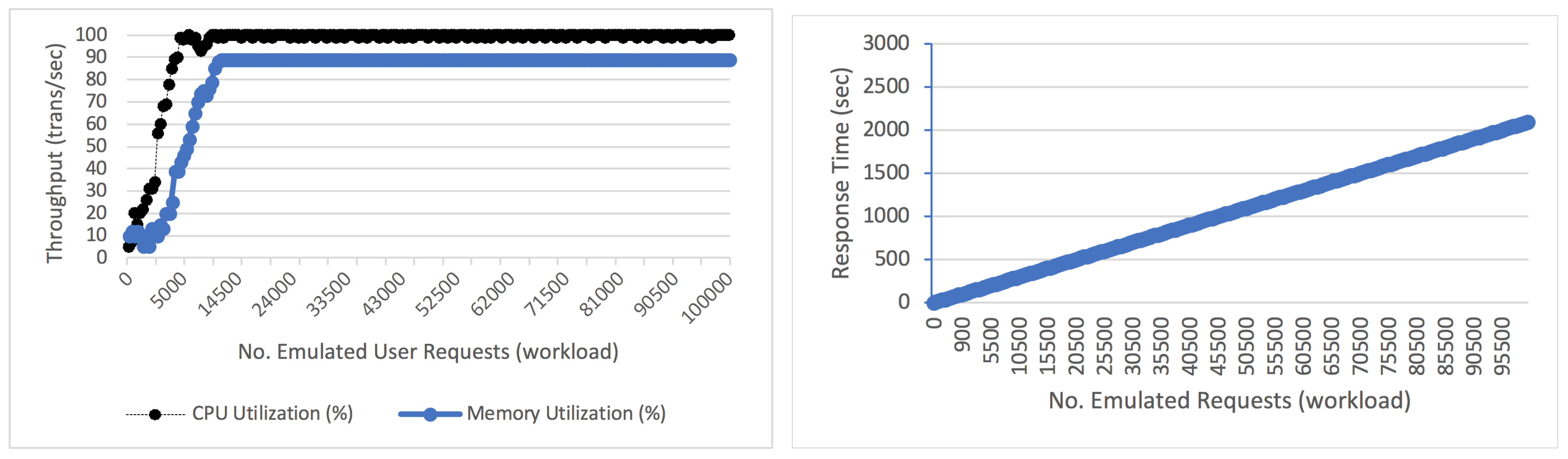
For the workload, we generate 100,000 requests at container level. To model the correlation between the workload and container performance/resource utilization metrics, we estimate Spearman’s Ranked Correlation between the number of emulated user requests waiting in queue and the collected parameters from the monitored metrics to verify if such performance variation is associated with the emulated user requests. As shown in Figure 7 (left), the throughput increases when the number of requests increases, then it remains constant. This means that the utilization of CPU and memory reached a bottleneck at 100% and 89% with the increasing number of user requests that reached 4500 and 10,500 req/s, respectively. On the other hand, the response time keeps increasing with the increasing number of requests as shown in Figure 7 (right). The results demonstrate that dynamic workload has a strong impact on the container metrics as the monitored container is unable to process more than those requests.
We notice that a linear relationship between the number of user requests and resource utilization before resource contention in each user transaction behaviour pattern. We calculate the correlation between the monitored metric and the number of user requests. We obtain a strong correlation of 0.4202 between the two variables, which confirms that the number of requests influences performance.
5.4. A Comparative Evaluation of Anomaly Detection and Identification
We evaluate the HHMM detection and identification in comparison to other approaches.
5.4.1. The Assessment of Anomaly Detection
The model performance is compared against other anomaly detection techniques like the dynamic bayesian network (DBN) and the hierarchical temporal memory (HTM). To evaluate the effectiveness of anomaly detection, five common measures [34] in anomaly detection are used:
- Precision is the ratio of correctly detected anomaly to the sum of correctly and incorrectly detected anomalies. High precision indicates the model correctly detects anomalous behaviour.
- Recall measures the completeness of correctly detected anomalies to the total number of detected anomalies that are actually defective. Higher recall indicates that fewer anomaly cases are undetected.
- F1-score measures the detection accuracy. It considers both precision and recall of the detection to compute the F1-score with values from [0–1]. The higher the value, the better the result.
- False Alarm Rate (FAR) is the number of normal components, which have been detected as anomalous (values in [0–1]). A lower FAR value indicates the model effectively detects anomalies.
The True Positive (TP) means the detection/identification of anomalies is correct. Similarly, False Positive (FP) means the detection/identification of anomalies is incorrect as the model detects/identifies the normal behaviour as anomalous. False Negative (FN) means the model cannot detect/identify some anomalies, and thus does not produce the correct detection/identification as it interprets the anomaly behaviour as normal behaviour. True Negative (TN) means the model can correctly detect and identify normal behaviour as normal.
The model is trained on the datasets in Table 8. The HHMM, the DBN and the HTM are trained on 3 nodes that are needed to deploy the TPC-W benchmark. The results show that both the HHMM and the HTM achieve good results on datasets A and B. While the results of the DBN worsened on dataset B and C, it gave satisfying results on dataset A. For dataset C, the algorithm performance significantly decreased. The results show that the HHMM and the HTM model detect anomalous behaviour with good results compared to the DBN on small and moderate datasets.
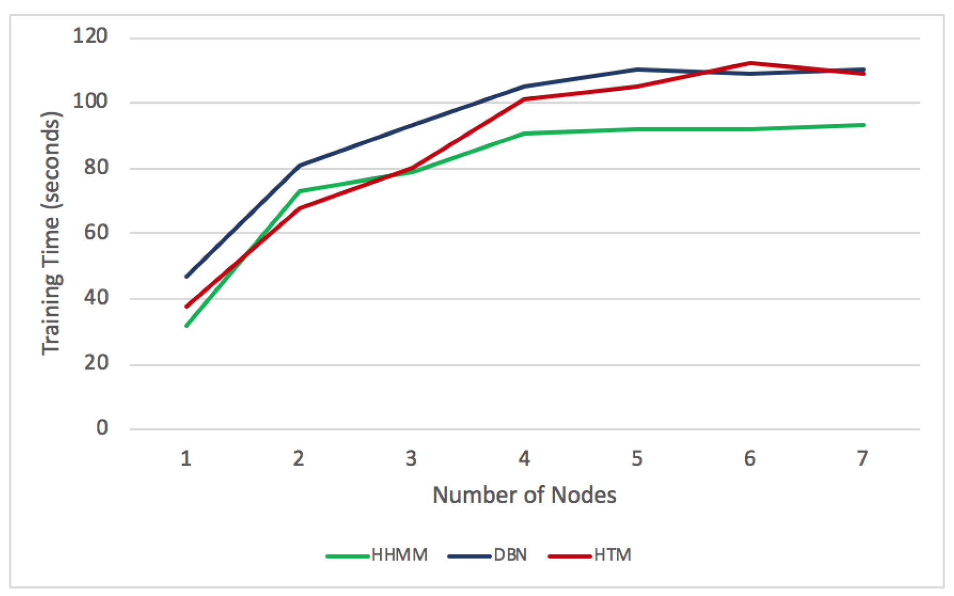
Moreover, we train the models on different numbers of nodes with anomaly observation sequences of length 100. We inject one type of anomaly (e.g., CPU hog). Here, we run one iteration for each model. As shown in Figure 8, the training time for the HHMM, the DBN and the HTM are increased as we increase the number of nodes for training the models. For example, with one node, the training time for the HHMM is 32 s, for DBN is 47 s, and for HTM is 38 s. With 4 nodes, the training time for the HHMM, the DBN and the HTM increase to 91, 105 and 101 s respectively. However, the training time slightly increases with 5, 6 and 7 nodes. For each node, we measure the accuracy of the detection as shown in Figure 9. The accuracy achieved in the HHMM is 95%, whereas for the DBN and the HTM, the accuracy increased to 89% and 90% respectively.
5.4.2. The Assessment of Anomaly Identification
In order to identify the location and reason of anomalous behaviour, different anomalies are injected one at a time at different system levels. Also, various workloads with different configurations are generated at container level. The performance data of the components under test differ from one experiment to another. Consequently, we use the Euclidean distance to measure the similarity between the sequences generated from the components. The component with the furthest distance from others is considered anomalous. We consider the anomaly root cause identification successful if any of the injected anomalies is related to the same resource (e.g., CPU, memory) as the injected anomaly. Otherwise, we consider the anomaly root-cause identification a failure, if the value of Accuracy of Identification (AI) is high.
- Accuracy of Identification (AI): measures the completeness of the correctly identified anomalies with respect to the total number of anomalies in a given dataset. The higher the value, the more correct the identification made by the model.
- Number of Correctly Identified Anomaly (CIA): It is the percentage of correct identified anomalies (NCIA) out of the total set of identifications, which is the number of correct Identification (NCIA) + the number of incorrect Identifications (NICI)). A higher value indicates the model is correctly identified anomalous component.
- Number of Incorrectly Identified Anomaly (IIA): is the percentage of identified components that represent an anomaly, but are misidentified as normal by the model. A lower value indicates that the model correctly identified anomalous components.
- False Alarm Rate (FAR): is the number of normal identified components, which have been misclassified as anomalous by the model.
As shown in Table 9, the HHMM and the HTM achieve promising results for the identification of anomaly, while the result of the DBN for the CIA decreased with approximately 7% compared to the HHMM and 6% to the HTM. Both the HHMM and the HTM show higher identification accuracy as they are able to identify temporal anomalies in the dataset. The result confirms that the HHMM is able to link observed failure to its hidden workload.
We also compare the accuracy of each algorithm in correctly identifying the root cause with the number of samples (the number of detected anomalies in a dataset). As shown in Figure 10, the root cause is identified correctly by the HHMM with an accuracy of around 98%. The HHMM gives satisfying results on different samples. For the HTM, its accuracy fluctuates with the increasing numbers of samples, reaching 97% with 100 samples. It should be noted that the HHMM achieves optimal results with 90 and 100 samples, while the DBN and the HTM achieve optimal results with 70–90 and 90 samples only, respectively.
5.5. Comparison with Other Monitoring Tools
In order to further validate the model, we conduct another experiment, shown in Table 10, by comparing the HHMM detection and identification with the Zabbix (https://www.zabbix.com/) and the Dynatrace (https://www.dynatrace.com/) monitoring tools to avoid threats to validity arising from the tool selection. The validation focuses on measuring Detection and Identification Latency (DIL) achieved using each of the monitoring tools. The DIL refers to the difference between the time of injection and the moment when the anomaly is identified in seconds. We focus on the anomaly behaviour of CPU hog and memory leak. The detection and identification of the anomaly behaviours achieved after the injection of anomaly with few seconds. After a few seconds (e.g., 25 s) from the CPU hog injection, the number of unprocessed user requests increases from 34 to 110 requests with lowest response time = 357 ms. For the Memory leak, the number of unprocessed user requests increases from 21 to 78 requests with lowest response time = 509 ms. Table 10 shows that our proposed framework provides the shortest detection latency for both factors compared to other monitoring tools.
5.6. Discussion
The experimental results show the effectiveness of our mechanism. However, some potential limitations shall be discussed here.
While at cluster level, we restrict architectures to 3 nodes, inside each node the number of containers is not restricted and these can be added freely. Thus, the mechanism to expand is built in.
In other works [35,36,37,38], we have implemented and experimentally evaluated 8-node cluster architectures, with 3 types of containers (orchestration, service provider, service consumer) in different architectural settings. Our observation from these experiments was that taking into account specific architecture configuration will not result in sufficiently generic results. Thus, in our case analysis here, we have focused on client-server type dependencies between container resources to determine anomalies and their root causes.
We used 150 min as the training time for the experiments. While some reductions is possible, in some real-time environments, this limits the applicability. We add this concern as future work.
6. Conclusions and Future Work
Monitoring of containers and nodes hosted in clusters, i.e., managed distributed systems, opens many challenges in terms of reliability and performance management at run-time. This paper explores the use of HHMMs to detect and identify anomalous behaviour found in container and node workloads. We focus on measuring response time and resource utilization of containers and nodes to detect anomalous behaviour and to identify their root cause.
For the evaluation, we derive workload variations of containers and nodes over different time scales in the context of the HHMM. The conducted experiments have demonstrated the effectiveness and efficiency of the proposed framework in tracing anomalous behaviours to their root causes within components over different workload intensity periods.
In the future, we plan to complement the framework by providing recovery actions to be applied to different types of identified anomalies. So far, the framework only focuses on some common performance and load-related anomalies. In the future, we will include more anomaly scenarios for different scenarios and architectures [2,36], and we will handle more metrics to capture more cases, but still maintaining accuracy.
An essential step was to link observable anomalies for the use to underlying root causes at the resource level. The next step would be to link anomalies not only to direct service-level failures, but also to a more semantic level [39,40,41], involving the wider objectives and goals of a user when using the application in question, i.e., to fulfill a specific task. A challenging example here would be educational technology systems [42,43,44,45,46] that we have been developing in the past, since the failure to attain more abstract goals might be linked to anomalies in the system performance.
Author Contributions
The authors have both been involved in the design the models, implementation the algorithms, and performing the evaluation. The work is the outcome of a PhD thesis by the first author, with the second author involved as the supervisor in all activities. All authors have read and agreed to the published version of the manuscript.
Funding
This research received no external funding.
Conflicts of Interest
The authors declare that they have no conflict of interest.
Abbreviations
The following abbreviations are used in this manuscript:
| HMM | Hidden Markov Model |
| HHMM | Hierarchical Hidden Markov Model |
| MAPE-K | Monitor Analysis Plan Execute - Knowledge |
| DD | Dissociation Degree |
| DBN | Dynamic Bayesian Network |
| HTM | Hierarchical Temporal Memory |
| IIA | Incorrect Identified Anomaly |
| CIA | Correct Identified Anomaly |
| NCIA | Number of Correct Identification Anomaly |
| NICI | Number of Incorrect Identification |
| FAR | False Alarm Rate |
| DIL | Detection and Identification Latency |
References
- Pahl, C.; Jamshidi, P.; Zimmermann, O. Architectural principles for cloud software. ACM Trans. Internet Technol. (TOIT) 2018, 18, 17. [Google Scholar] [CrossRef]
- Taibi, D.; Lenarduzzi, V.; Pahl, C. Architecture Patterns for a Microservice Architectural Style. In Communications in Computer and Information Science; Springer: New York, NY, USA, 2019. [Google Scholar]
- Taibi, D.; Lenarduzzi, V.; Pahl, C. Architectural Patterns for Microservices: A Systematic Mapping Study. In Proceedings of the CLOSER Conference, Madeira, Portugal, 19–21 March 2018; pp. 221–232. [Google Scholar]
- Jamshidi, P.; Pahl, C.; Mendonca, N.C. Managing uncertainty in autonomic cloud elasticity controllers. IEEE Cloud Comput. 2016, 3, 50–60. [Google Scholar] [CrossRef]
- Mendonca, N.C.; Jamshidi, P.; Garlan, D.; Pahl, C. Developing Self-Adaptive Microservice Systems: Challenges and Directions. IEEE Softw. 2020. [Google Scholar] [CrossRef] [Green Version]
- Gow, R.; Rabhi, F.A.; Venugopal, S. Anomaly detection in complex real world application systems. IEEE Trans. Netw. Serv. Manag. 2018, 15, 83–96. [Google Scholar] [CrossRef]
- Alcaraz, J.; Kaaniche, M.; Sauvanaud, C. Anomaly Detection in Cloud Applications: Internship Report. Machine Learning [cs.LG]. 2016. hal-01406168. Available online: https://hal.laas.fr/hal-01406168 (accessed on 15 December 2019).
- Du, Q.; Xie, T.; He, Y. Anomaly Detection and Diagnosis for Container-Based Microservices with Performance Monitoring. In Proceedings of the International Conference on Algorithms and Architectures for Parallel Processing, Guangzhou, China, 15–17 November 2018; pp. 560–572. [Google Scholar]
- Wang, T.; Xu, J.; Zhang, W.; Gu, Z.; Zhong, H. Self-adaptive cloud monitoring with online anomaly detection. Future Gener. Comput. Syst. 2018, 80, 89–101. [Google Scholar] [CrossRef]
- Düllmann, T.F. Performance Anomaly Detection in Microservice Architectures under Continuous Change. Master’s Thesis, University of Stuttgart, Stuttgart, Germany, 2016. [Google Scholar]
- Wert, A. Performance Problem Diagnostics by Systematic Experimentation. Ph.D. Thesis, KIT, Karlsruhe, Germany, 2015. [Google Scholar]
- Barford, P.; Duffield, N.; Ron, A.; Sommers, J. Network performance anomaly detection and localization. In Proceedings of the IEEE INFOCOM 2009, Rio de Janeiro, Brazil, 19–25 April 2009; pp. 1377–1385. [Google Scholar] [CrossRef] [Green Version]
- Pahl, C.; Brogi, A.; Soldani, J.; Jamshidi, P. Cloud container technologies: A state-of-the-art review. IEEE Trans. Cloud Comput. 2018, 7, 677–692. [Google Scholar] [CrossRef]
- Lawrence, H.; Dinh, G.H.; Williams, A.; Ball, B. Container Monitoring and Management. 2018. Available online: https://docs.broadcom.com/docs/container-monitoring-ebook (accessed on 15 December 2019).
- Taylor, T. 6 Container Performance KPIs You Should Be Tracking to Ensure DevOps Success. 2018. Available online: https://www.devopsdigest.com/6-container-performance-kpis-you-should-be-tracking-to-ensure-devops-success (accessed on 15 December 2019).
- Fine, S.; Singer, Y.; Tishby, N. The hierarchical hidden markov model: Analysis and applications. Mach. Learn. 1998, 32, 41–62. [Google Scholar] [CrossRef] [Green Version]
- Sorkunlu, N.; Chandola, V.; Patra, A. Tracking system behavior from resource usage data. In Proceedings of the IEEE International Conference on Cluster Computing, ICCC, Honolulu, HI, USA, 5–8 September 2017; Volume 2017, pp. 410–418. [Google Scholar] [CrossRef]
- Agrawal, B.; Wiktorski, T.; Rong, C. Adaptive anomaly detection in cloud using robust and scalable principal component analysis. In Proceedings of the 2016 15th International Symposium on Parallel and Distributed Computing (ISPDC), Fuzhou, China, 8–10 July 2016; pp. 100–106. [Google Scholar] [CrossRef]
- Magalhães, J.P. Self-Healing Techniques for Web-Based Applications. Ph.D. Thesis, University of Coimbra, Coimbra, Portugal, 2013. [Google Scholar]
- Kozhirbayev, Z.; Sinnott, R.O. A performance comparison of container-based technologies for the Cloud. Future Gener. Comput. Syst. 2017, 68, 175–182. [Google Scholar] [CrossRef]
- Peiris, M.; Hill, J.H.; Thelin, J.; Bykov, S.; Kliot, G.; Konig, C. PAD: Performance anomaly detection in multi-server distributed systems. In Proceedings of the 2014 IEEE 7th International Conference on Cloud Computing, Anchorage, AK, USA, 27 June–2 July 2014; Volume 7, pp. 769–776. [Google Scholar] [CrossRef]
- Sukhwani, H. A Survey of Anomaly Detection Techniques and Hidden Markov Model. Int. J. Comput. Appl. 2014, 93, 26–31. [Google Scholar] [CrossRef]
- Ge, N.; Nakajima, S.; Pantel, M. Online diagnosis of accidental faults for real-time embedded systems using a hidden markov model. Simulation 2016, 91, 851–868. [Google Scholar] [CrossRef] [Green Version]
- Brogi, G. Real-Time Detection of Advanced Persistent Threats Using Information Flow Tracking and Hidden Markov Models. Ph.D. Thesis, Conservatoire National des Arts et Métiers, Paris, France, 2018. [Google Scholar]
- Samir, A.; Pahl, C. A Controller Architecture for Anomaly Detection, Root Cause Analysis and Self-Adaptation for Cluster Architectures. In Proceedings of the International Conference on Adaptive and Self-Adaptive Systems and Applications, Venice, Italy, 5–9 May 2019; pp. 75–83. [Google Scholar]
- Samir, A.; Pahl, C. Self-Adaptive Healing for Containerized Cluster Architectures with Hidden Markov Models. In Proceedings of the 2019 Fourth International Conference on Fog and Mobile Edge Computing (FMEC), Rome, Italy, 10–13 June 2019. [Google Scholar]
- Samir, A.; Pahl, C. Detecting and Predicting Anomalies for Edge Cluster Environments using Hidden Markov Models. In Proceedings of the Fourth IEEE International Conference on Fog and Mobile Edge Computing, Rome, Italy, 10–13 June 2019; pp. 21–28. [Google Scholar]
- Chis, T. Sliding hidden markov model for evaluating discrete data. In European Workshop on Performance Engineering; Springer: Berlin/Heidelberg, Germany, 2014. [Google Scholar]
- Bachiega, N.G.; Souza, P.S.; Bruschi, S.M.; De Souza, S.D.R. Container-based performance evaluation: A survey and challenges. In Proceedings of the 2018 IEEE International Conference on Cloud Engineering, IC2E 2018, Orlando, FL, USA, 17–20 April 2018; pp. 398–403. [Google Scholar] [CrossRef]
- La Rosa, A. Docker Monitoring: Challenges Introduced by Containers and Microservices. 2018. Available online: https://pandorafms.com/blog/docker-monitoring/ (accessed on 15 December 2019).
- Al-Dhuraibi, Y.; Paraiso, F.; Djarallah, N.; Merle, P. Elasticity in cloud computing: State of the art and research challenges. IEEE Trans. Serv. Comput. 2017, 11, 430–447. [Google Scholar] [CrossRef] [Green Version]
- Spearman’s Rank Correlation Coefficient Rs and Probability (p) Value Calculator; Barcelona Field Studies Centre: Barcelona, Spain, 2019.
- Josefsson, T. Root-Cause Analysis Through Machine Learning in the Cloud. Master’s Thesis, Upsala Univ., Uppsala, Sweden, 2017. [Google Scholar]
- Markham, K. Simple Guide to Confusion Matrix Terminology 2014. Available online: https://www.dataschool.io/simple-guide-to-confusion-matrix-terminology/ (accessed on 15 December 2019).
- Pahl, C.; El Ioini, N.; Helmer, S.; Lee, B. An architecture pattern for trusted orchestration in IoT edge clouds. In Proceedings of the Third International Conference on Fog and Mobile Edge Computing, FMEC, Barcelona, Spain, 23–26 April 2018; pp. 63–70. [Google Scholar]
- Scolati, R.; Fronza, I.; El Ioini, N.; Samir, A.; Pahl, C. A Containerized Big Data Streaming Architecture for Edge Cloud Computing on Clustered Single-Board Devices. In Proceedings of the 10th International Conference on Cloud Computing and Services Science, Prague, Czech Republic, 7–9 May 2020; pp. 68–80. [Google Scholar]
- Von Leon, D.; Miori, L.; Sanin, J.; El Ioini, N.; Helmer, S.; Pahl, C. A performance exploration of architectural options for a middleware for decentralised lightweight edge cloud architectures. In Proceedings of the CLOSER Conference, Madeira, Portugal, 19–21 March 2018. [Google Scholar]
- Von Leon, D.; Miori, L.; Sanin, J.; El Ioini, N.; Helmer, S.; Pahl, C. A Lightweight Container Middleware for Edge Cloud Architectures. In Fog and Edge Computing: Principles and Paradigms; John Wiley & Sons, Inc.: Hoboken, NJ, USA, 2019; pp. 145–170. [Google Scholar]
- Pahl, C. An ontology for software component matching. In Proceedings of the International Conference on Fundamental Approaches to Software Engineering, Warsaw, Poland, 7–11 April 2003; pp. 6–21. [Google Scholar]
- Pahl, C. Layered ontological modelling for web service-oriented model-driven architecture. In Proceedings of the European Conference on Model Driven Architecture—Foundations and Applications, Nuremberg, Germany, 7–10 November 2005. [Google Scholar]
- Javed, M.; Abgaz, Y.M.; Pahl, C. Ontology change management and identification of change patterns. J. Data Semant. 2013, 2, 119–143. [Google Scholar] [CrossRef] [Green Version]
- Kenny, C.; Pahl, C. Automated tutoring for a database skills training environment. In Proceedings of the ACM SIGCSE Symposium 2005, St.Louis, MO, USA, 23–27 February 2005; pp. 58–64. [Google Scholar]
- Murray, S.; Ryan, J.; Pahl, C. A tool-mediated cognitive apprenticeship approach for a computer engineering course. In Proceedings of the 3rd IEEE International Conference on Advanced Technologies, Athens, Greece, 9–11 July 2003; pp. 2–6. [Google Scholar]
- Pahl, C.; Barrett, R.; Kenny, C. Supporting active database learning and training through interactive multimedia. ACM SIGCSE Bull. 2004, 36, 27–31. [Google Scholar] [CrossRef]
- Lei, X.; Pahl, C.; Donnellan, D. An evaluation technique for content interaction in web-based teaching and learning environments. In Proceedings of the 3rd IEEE International Conference on Advanced Technologies, Athens, Greece, 9–11 July 2003; pp. 294–295. [Google Scholar]
- Melia, M.; Pahl, C. Constraint-based validation of adaptive e-learning courseware. IEEE Trans. Learn. Technol. 2009, 2, 37–49. [Google Scholar] [CrossRef] [Green Version]
Figure 1.
Anomaly detection and localization based on HHMM.

Figure 2.
Anomaly detection-identification framework.

Figure 3.
CPU hog detection using HHMM fo the whole system.

Figure 4.
Memory leak detection using HHMM for the whole system.

Figure 5.
CPU hog detection using HHMM for components.

Figure 6.
Memory leak detection using HHMM for components.

Figure 7.
Workload–throughput (left) and response time (right) over No. of user requests.

Figure 8.
Comparative training time of HHMM, DBN and HTM.

Figure 9.
Comparative detection accuracy of HHMM, DBN and HTM.

Figure 10.
Accuracy of anomaly root cause identification.


Table 1.
Monitoring metrics.
| Metric Name | Description |
|---|---|
| CPU Usage | CPU utilization for each container and node |
| CPU Request | CPU request in millicores |
| Resource Saturation | The amount of work a CPU/memory cannot serve and waiting in queue |
| Memory Usage | Occupied memory of the container |
| Memory Request | Memory request in bytes |
| Node CPU Capacity | Total CPU capacity of cluster nodes |
| Node Memory Capacity | Total memory capacity of cluster nodes |
Table 2.
Hardware and software specification used in the experiment.
| Components | Settings |
|---|---|
| CPU | 2.7GH_z Intel Cores i5 |
| Disk Space | 1TB |
| Memory | 8 GB DDR3 |
| Operating System | MacOS |
| Application | R |
| Dataset | TPC-W benchmark |
Table 3.
Configuration of cluster nodes and container.
| Components | Settings |
|---|---|
| Number of Nodes | 3 |
| Container no. | 4 |
| Number of CPUs | 3 |
| HD | 512 GB |
| RAM | 2 GB |
| Guest OS | Linux |
| Orchestration Tool | Docker and Kubernetes |
Table 4.
Workload configuration parameters.
| Parameter Name | Description | Value |
|---|---|---|
| EB | Emulate a client by sending and receiving requests | rbe.EBTPCW1Factory |
| CUST | Generate random number of customers | 15,000 |
| Ramp-up | Time between sending requests | 600 s |
| ITEM | Number of items in database | 100,000 |
| Number of Requests | Number of requests generated per second | 30–100,000 request/s |
Table 5.
Injected anomalies.
| Resource | Fault Type | Fault Description | Injection Operation |
|---|---|---|---|
| CPU | CPU hog | Consume all CPU cycles for a container | Employing infinite loops that consumes all CPU cycle |
| Memory | Memory leak | Exhausts a container memory | Injected anomalies to utilize all memory capacity |
| Workload | Workload Contention | Generate increasing number of requests that saturate the component resources | Emulate user requests using Remote Browser Emulators in TPC-W benchmark |
Table 6.
CPU hog detection using HHMM.
| Components | Injection Time (Interval) | Detection Time (Interval) | Detection Period (Interval) |
|---|---|---|---|
| C3.1 | 100 | 140 | 40 |
| C3.2 | 250 | 340 | 90 |
| C3.3 | 400 | 460 | 60 |
| C3.4 | 550 | 620 | 70 |
| N2.1 | 700 | 760 | 60 |
| N2.3 | 850 | 950 | 100 |
Table 7.
Memory leak detection using HHMM.
| Components | Injection Time (Interval) | Detection Time (Interval) | Detection Period (Interval) |
|---|---|---|---|
| C3.1 | 100 | 140 | 40 |
| C3.2 | 250 | 320 | 70 |
| C3.3 | 400 | 490 | 90 |
| C3.4 | 550 | 650 | 100 |
| N2.1 | 700 | 760 | 60 |
| N2.3 | 850 | 950 | 100 |
Table 8.
Validation results of three datasets.
| Datasets | Metrics | HHMM | DBN | HTM |
|---|---|---|---|---|
| A = 650 | Precision | 0.95 | 0.94 | 0.95 |
| Recall | 0.96 | 0.96 | 0.95 | |
| F1-score | 0.95 | 0.95 | 0.95 | |
| FAR | 0.19 | 0.21 | 0.28 | |
| B = 861 | Precision | 0.96 | 0.91 | 0.95 |
| Recall | 0.94 | 0.84 | 0.91 | |
| F1-score | 0.95 | 0.87 | 0.93 | |
| FAR | 0.27 | 0.46 | 0.31 | |
| C = 1511 | Precision | 0.87 | 0.64 | 0.87 |
| Recall | 0.93 | 0.83 | 0.94 | |
| F1-score | 0.90 | 0.72 | 0.90 | |
| FAR | 0.31 | 0.47 | 0.33 |
Table 9.
Assessment of identification.
| Metrics | HHMM | DBN | HTM |
|---|---|---|---|
| AI | 0.94 | 0.84 | 0.94 |
| CIA | 94.73% | 87.67% | 93.94% |
| IIA | 4.56% | 12.33% | 6.07% |
| FAR | 0.12 | 0.26 | 0.17 |
Table 10.
Anomaly detection and identification latency (DIL).
| Anomaly Behaviour | Zabbix | Dynatrace | Framework |
|---|---|---|---|
| CPU Hog | 410 | 408 | 398 |
| Memory Leak | 520 | 522 | 515 |
© 2020 by the authors. Licensee MDPI, Basel, Switzerland. This article is an open access article distributed under the terms and conditions of the Creative Commons Attribution (CC BY) license (http://creativecommons.org/licenses/by/4.0/).
Share and Cite
MDPI and ACS Style
Samir, A.; Pahl, C. Detecting and Localizing Anomalies in Container Clusters Using Markov Models. Electronics 2020, 9, 64. https://0-doi-org.brum.beds.ac.uk/10.3390/electronics9010064
AMA Style
Samir A, Pahl C. Detecting and Localizing Anomalies in Container Clusters Using Markov Models. Electronics. 2020; 9(1):64. https://0-doi-org.brum.beds.ac.uk/10.3390/electronics9010064
Chicago/Turabian StyleSamir, Areeg, and Claus Pahl. 2020. "Detecting and Localizing Anomalies in Container Clusters Using Markov Models" Electronics 9, no. 1: 64. https://0-doi-org.brum.beds.ac.uk/10.3390/electronics9010064
Note that from the first issue of 2016, this journal uses article numbers instead of page numbers. See further details here.