An Efficient Numerical Formulation for Wave Propagation in Magnetized Plasma Using PITD Method

Abstract

A modified precise-integration time-domain (PITD) formulation is presented to model the wave propagation in magnetized plasma based on the auxiliary differential equation (ADE). The most prominent advantage of this algorithm is using a time-step size which is larger than the maximum value of the Courant–Friedrich–Levy (CFL) condition to achieve the simulation with a satisfying accuracy. In this formulation, Maxwell’s equations in magnetized plasma are obtained by using the auxiliary variables and equations. Then, the spatial derivative is approximated by the second-order finite-difference method only, and the precise integration (PI) scheme is used to solve the resulting ordinary differential equations (ODEs). The numerical stability and dispersion error of this modified method are discussed in detail in magnetized plasma. The stability analysis validates that the simulated time-step size of this method can be chosen much larger than that of the CFL condition in the finite-difference time-domain (FDTD) simulations. According to the numerical dispersion analysis, the range of the relative error in this method is ${10}^{-6}$ to $5\times {10}^{-4}$ when the electromagnetic wave frequency is from 1 GHz to 100 GHz. More particularly, it should be emphasized that the numerical dispersion error is almost invariant under different time-step sizes which is similar to the conventional PITD method in the free space. This means that with the increase of the time-step size, the presented method still has a lower computational error in the simulations. Numerical experiments verify that the presented method is reliable and efficient for the magnetized plasma problems. Compared with the formulations based on the FDTD method, e.g., the ADE-FDTD method and the JE convolution FDTD (JEC-FDTD) method, the modified algorithm in this paper can employ a larger time step and has simpler iterative formulas so as to reduce the execution time. Moreover, it is found that the presented method is more accurate than the methods based on the FDTD scheme, especially in the high frequency range, according to the results of the magnetized plasma slab. In conclusion, the presented method is efficient and accurate for simulating the wave propagation in magnetized plasma.

1. Introduction

The simulations of the electromagnetic (EM) wave propagation in the magnetized plasma are attractive and have a wide range of applications, e.g., high frequency components, PCB design, microstrip antenna, and so on [1,2,3,4,5,6]. Recently, the finite-difference time-domain (FDTD) formulation is the most popular numerical tool in the full wave analysis, and widely used in the simulation of the magnetized plasma and other dispersive materials. The typical algorithms based on the FDTD method for modeling the dispersive material include the recursive convolution (RC) FDTD method [7,8], the auxiliary differential equation (ADE) FDTD method [9,10,11], and the Z-transform (ZT) FDTD method [12,13]. Unfortunately, the FDTD method has an inherent drawback on which the above methods are based, i.e., Courant–Friedrich–Levy (CFL) stability criterion, and it has limited the further applications of the FDTD method in the dispersive materials as the problem expands. Assume that the spatial mesh is very fine to obtain the satisfying accuracy, the CFL stability criterion indicates that the time-step size should be a small enough value to ensure the numerical results are convergent. It is easily seen that such a small time-step size leads to an increase of the iteration step and a higher computational memory requirement so as to decrease the effectiveness of the FDTD calculation significantly and sometimes increase the accumulated error of the simulation.

Prompted by the aforementioned reasons, a number of time-domain algorithms, which have looser stability conditions, are presented to improve the efficiency of the FDTD simulations, e.g., the alternating-direction implicit FDTD (ADI-FDTD) method [14,15], the locally-one-dimensional (LOD) FDTD method [16,17,18], the precise-integration time-domain (PITD) method [19], and so on. Therein, the ADI-FDTD method is established by the alternating-direction implicit technique, and it is implicit and has complex iterative formulas. The LOD-FDTD method, which is presented by Shibayama, et al., is based on both the locally-one-dimensional scheme and the split time step technique. Compared with the ADI-FDTD method, the LOD-FDTD method is more efficient because it has fewer arithmetical operations. Here, we know both the ADI-FDTD and LOD-FDTD methods are unconditional stable to solve the EM wave problems. This means that the CFL condition has no restraint on the time step, and the efficiency of the simulation can be improved significantly by employing a larger time step. Meanwhile, the numerical dispersion errors of the ADI-FDTD method and the LOD-FDTD method are comparable and similar. It should be emphasized that the computational errors of these two methods increase rapidly which leads to the unanticipated results when the time step is increased as shown in the following description. In recent years, the ADI-FDTD method and the LOD-FDTD method were also generalized to the application of the dispersive materials [20,21].

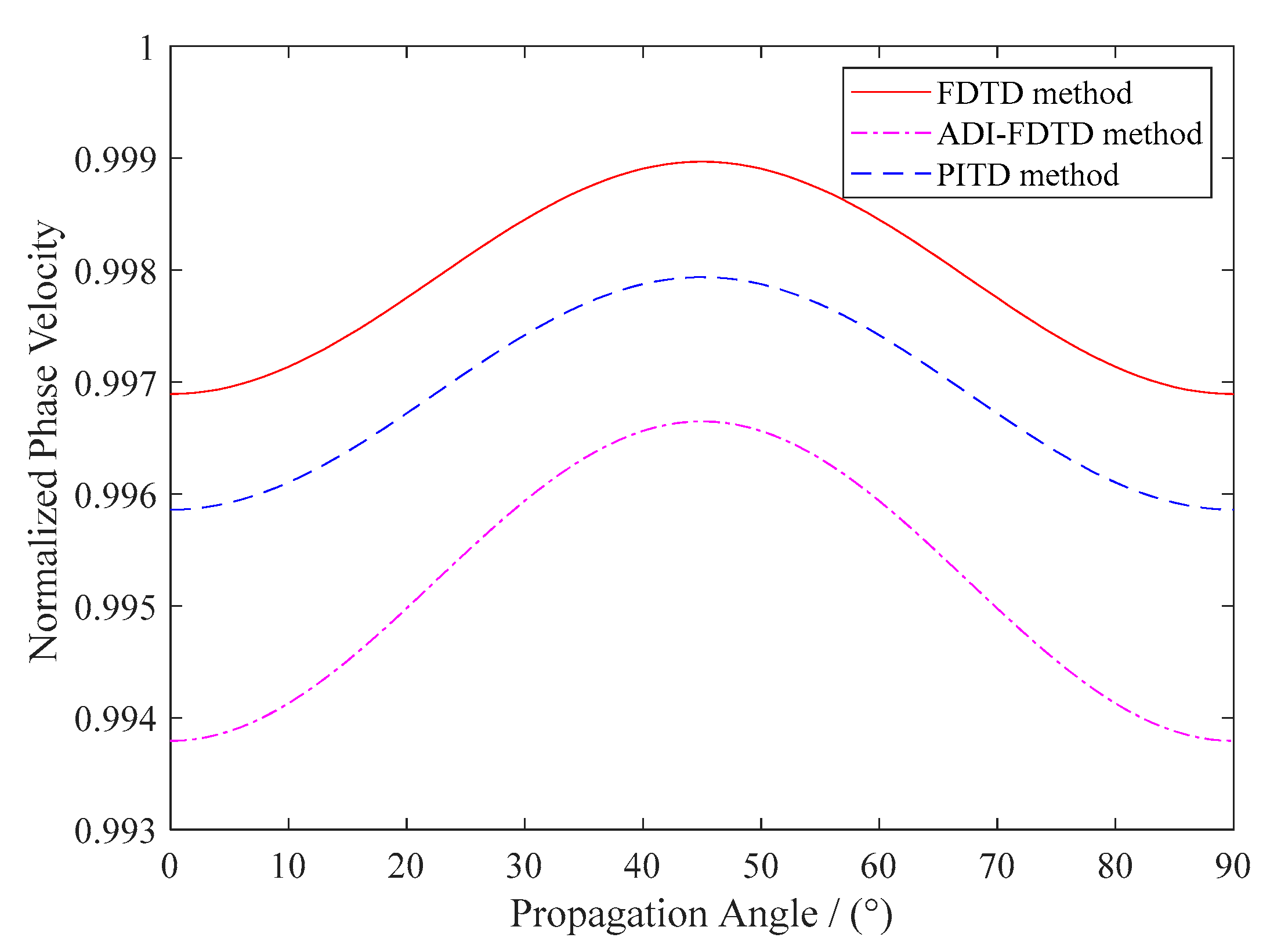
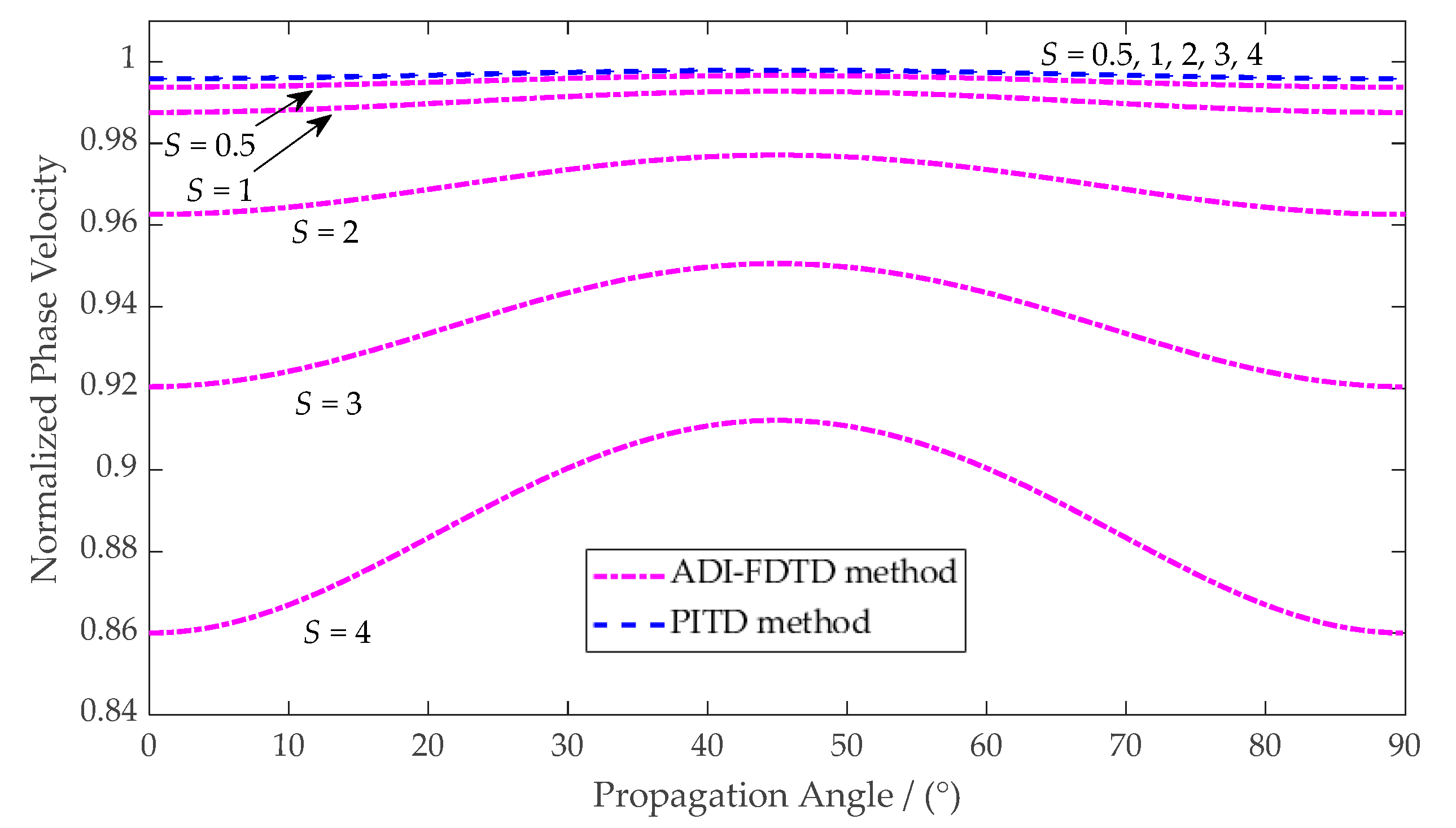
The PITD method, which is presented by Ma, et al., has been used to solve Maxwell’s equations in free space, lossy space, and unmagnetized plasma [19,22,23]. Although the PITD method is not unconditionally stable, it can still employ a time step which is much larger than the maximum value allowed by the CFL stability condition in the FDTD method [24]. Moreover, in contrast to the two unconditional stable methods mentioned above, the dispersion error of the PITD method is almost invariant when the time step is increased. This means that the PITD method can maintain a satisfactory computational accuracy when the time step is increased [25,26], and it makes the PITD method more suitable for the electrically large EM problems. Here, we take the ADI-FDTD method as the example. Figure 1 shows the numerical velocity of the FDTD, PITD, and ADI-FDTD methods with respect to the propagation angle when the Courant number is S = 0.5. It is found that the numerical dispersion error of the PITD method is larger than that of the FDTD method, but smaller than that of the ADI-FDTD method. Figure 2 shows the numerical velocity of the PITD method and the ADI-FDTD method versus the propagation angle under different Courant numbers. With the increase of the Courant number, the numerical dispersion error of the ADI-FDTD method is increased rapidly, however, the numerical dispersion error of the PITD method is still nearly invariant.

Due to the advantages mentioned above, the PITD method is a promising approach to model the EM wave propagation in magnetized plasma efficiently. The resulting Maxwell’s equations of magnetized plasma are firstly obtained by employing the auxiliary variables and equations related to the current density. Then, the second-order accurate finite-difference formulation is used to approximate the spatial derivative in the presented method, and several ordinary differential equations (ODEs) with respect to the time derivative are obtained directly. Finally, we use the PI scheme to solve the ODEs. After establishing the modified PITD method in magnetized plasma, the stability condition and the dispersion error are analyzed numerically. The stability analysis verifies that the numerical stability criterion of the presented method in magnetized plasma is much looser than the CFL stability condition of the FDTD methods so as to increase the maximum allowable time step, and the numerical dispersion errors are almost invariant when the time-step size is increased. Thus, this method has the potential to balance both the efficiency and the accuracy. The magnetized plasma slab and the magnetized plasma filled cavity are simulated to validate that the modified PITD method in the paper is reliable and efficient. The analyses of the numerical results indicate that the presented method can provide an evident reduction of the execution time by using a larger simulated time step, meanwhile, the computational error of the presented algorithm is also lower than those of the formulations based on the FDTD scheme, especially in the high frequency range.

The rest of this paper is organized as follows. The formulation of the presented method is introduced in Section 2. The stability analysis and the dispersion analysis are discussed numerically in Section 3. Numerical results are simulated to verify the efficiency and the accuracy of the presented algorithm in Section 4. Finally, conclusions are drawn in Section 5.

2. Formulations

2.1. Resulting Maxwell’s Equations of Magnetized Plasma

The curl Maxwell’s equations for describing the magnetized plasma problem is firstly established by employing the auxiliary variables and equations related to the current density J(t). The resulting matrix form is shown as follows:

$$\frac{\partial }{\partial t}\left[\begin{array}{l}\mathbf{E}\left(t\right)\\ \mathbf{H}\left(t\right)\\ \mathbf{J}\left(t\right)\end{array}\right]=\left[\begin{array}{ccc}0& \frac{1}{{\epsilon }_0}\nabla \times & -\frac{1}{{\epsilon }_0}\\ -\frac{1}{{\mu }_0}\nabla \times & 0& 0\\ {\epsilon }_0{\omega }_p^2& 0& -\gamma +{\omega }_b\times \end{array}\right]\left[\begin{array}{l}\mathbf{E}\left(t\right)\\ \mathbf{H}\left(t\right)\\ \mathbf{J}\left(t\right)\end{array}\right],$$

(1)

where ω_p and γ are the natural angular frequency and the collision frequency, respectively; ω_b = eB₀/m is the electron cyclotron angular frequency, wherein B₀ is the applied magnetic field, e is the electric quantity, and m is the mass of the electron.

Assume that the applied magnetic field is z-direction in the following analysis, and Equation (1) can be expanded as follows:

$$\frac{\partial }{\partial t}\left[\begin{array}{l}{E}_x\\ E_y\\ E_z\\ H_x\\ H_y\\ H_z\\ J_x\\ J_y\\ J_z\end{array}\right]=\left[\begin{array}{ccccccccc}0& 0& 0& 0& -\frac{1}{{\epsilon }_0}\frac{\partial }{\partial z}& \frac{1}{{\epsilon }_0}\frac{\partial }{\partial y}& -\frac{1}{{\epsilon }_0}& 0& 0\\ 0& 0& 0& \frac{1}{{\epsilon }_0}\frac{\partial }{\partial z}& 0& -\frac{1}{{\epsilon }_0}\frac{\partial }{\partial x}& 0& -\frac{1}{{\epsilon }_0}& 0\\ 0& 0& 0& -\frac{1}{{\epsilon }_0}\frac{\partial }{\partial y}& \frac{1}{{\epsilon }_0}\frac{\partial }{\partial x}& 0& 0& 0& -\frac{1}{{\epsilon }_0}\\ 0& \frac{1}{{\mu }_0}\frac{\partial }{\partial z}& -\frac{1}{{\mu }_0}\frac{\partial }{\partial y}& 0& 0& 0& 0& 0& 0\\ -\frac{1}{{\mu }_0}\frac{\partial }{\partial z}& 0& \frac{1}{{\mu }_0}\frac{\partial }{\partial x}& 0& 0& 0& 0& 0& 0\\ \frac{1}{{\mu }_0}\frac{\partial }{\partial y}& -\frac{1}{{\mu }_0}\frac{\partial }{\partial x}& 0& 0& 0& 0& 0& 0& 0\\ {\epsilon }_0{\omega }_p^2& 0& 0& 0& 0& 0& -\gamma & -{\omega }_b& 0\\ 0& {\epsilon }_0{\omega }_p^2& 0& 0& 0& 0& {\omega }_b& -\gamma & 0\\ 0& 0& {\epsilon }_0{\omega }_p^2& 0& 0& 0& 0& 0& -\gamma \end{array}\right]\left[\begin{array}{l}{E}_x\\ E_y\\ E_z\\ H_x\\ H_y\\ H_z\\ J_x\\ J_y\\ J_z\end{array}\right].$$

(2)

Here, we know that in the formulations based on the FDTD scheme, both the spatial and time derivatives are discretized by using the finite difference technique to obtain a set of algebraic equations from the Maxwell’s equations. However, in the proposed PITD algorithm, only the spatial derivative is discretized, and several ODEs are obtained temporarily and written as matrix form:

$$\frac{\mathrm{d}\mathbf{Y}}{\mathrm{d}t}=\mathbf{HY}+\mathbf{g}(t),$$

(3)

where $Y={\left[E_x,E_y,E_z,H_x,H_y,H_z,J_x,J_y,J_z\right]}^{\mathrm{T}}$, the coefficient matrix H is determined by both the EM parameters of the medium and the spatial step of the simulation, and g(t) is an inhomogeneous term related to the excitations.

The analytical and discrete solutions of Equation (3) are:

$$\mathbf{Y}\left(t\right)=e^{\mathbf{H}t}\mathbf{Y}\left(0\right)+{\displaystyle {\int }_0^t{e}^{\mathbf{H}\left(t-\tau \right)}\mathbf{g}\left(\tau \right)\mathbf{d}\tau },$$

(4)

and

$${\mathbf{Y}}_{n+1}=T{\mathbf{Y}}_n+T^{n+1}{\displaystyle {\int }_{t_n}^{t_{n+1}}{e}^{-\tau \mathbf{H}}\mathbf{g}\left(\tau \right)\mathbf{d}\tau },$$

(5)

where ${\mathbf{Y}}_n=\mathbf{Y}\left(n\Delta t\right)$ is the discrete form of Y(t) and $T=\exp \left(H\Delta t\right)$ which can be calculated by the the PI technique.

2.2. PI Technique Review

The exponential matrix T is firstly reformulated as:

$$T={\left[\exp \left(Hs\right)\right]}^l,$$

(6)

where $s=\Delta t/l$, $l=2^N$, and $N$ is a preselected arbitrary integer. If $N$ is large enough, the interval of s will be extremely small. Then, the Taylor series expansion is employed to approximate $\exp \left(Hs\right)$ with a high precision as shown in the following:

$$\exp \left(Hs\right)\approx I+T_a,$$

(7)

where:

$$T_a=\left(Hs\right)+\frac{{\left(Hs\right)}^2}{2!}+\frac{{\left(Hs\right)}^3}{3!}+\frac{{\left(Hs\right)}^4}{4!},$$

(8)

and evidently,

$$T\approx {\left(I+T_a\right)}^l.$$

(9)

It should be noted that if T_a is added to the identity matrix I directly, T_a will be neglected because T_a is extremely small, which leads to a precision reduction of the exponential matrix. Therefore, it is evident that T_a should be operated in the process.

The matrix T is computed as follows:

$$T\approx {\left(I+T_a\right)}^l={\left(I+T_a\right)}^{2^N}={\left(I+T_a\right)}^{2^{N-1}}\times {\left(I+T_a\right)}^{2^{N-1}}=\cdot \cdot \cdot ,$$

(10)

and

$${\left(I+T_a\right)}^2=I+2T_a+T_a\times T_a.$$

(11)

Start with Equation (8) to compute T_a and then run the following instruction, the exponential matrix T can be calculated:

do. $i=1,N$

$$T_a=2T_a+T_a\times T_a.$$

(12)

end do

$$T=I+T_a.$$

(13)

Equations (8), (12), and (13) constitute the whole process of the PI technique to calculate the exponential matrix. Relying on the previous work, the simulated time step of the PITD method is much larger than the maximum allowable value of the CFL stability condition of the FDTD formulation in the lossless or lossy problems, which is very significant in the full wave analysis. For the magnetized plasma material, we believe the application of the PI technique can achieve the same effect and the following stability analysis and numerical experimentations will prove this point.

Furthermore, for the integration on the right-hand side of Equation (5), a linear variation of the term $\mathbf{g}\left(t\right)$ is assumed within the interval $\left(t_n,t_{n+1}\right)$, expressed as:

$$\mathbf{g}\left(t\right)={\mathbf{r}}_0+{\mathbf{r}}_1\left(t-t_n\right),$$

(14)

Substitute the above expression in the integration, we have the following recursive form solution:

$$Y_{n+1}=T\left[Y_n+M^{-1}(r_0+M^{-1}{r}_1)\right]-M^{-1}\left[r_0+M^{-1}{r}_1+r_1\Delta t\right].$$

(15)

In most cases, Equation (15) is unavailable directly since the matrix $M$ is noninvertible. To mitigate this problem, the three-points Gauss integral formula is adopted to calculate the integration in Equation (5), and the recurrence formula is obtained as follows:

$$\begin{gathered} Y_{n+1}=T{Y}_n+\frac{5\Delta t}{18}\exp \left[\left(\frac{\Delta t}{2}+\frac{\Delta t}{2}\sqrt{\frac{3}{5}}\right)H\right]\mathbf{g}\left(t_n+\frac{\Delta t}{2}-\frac{\Delta t}{2}\sqrt{\frac{3}{5}}\right) \\ +\frac{8\Delta t}{18}\exp \left[\frac{\Delta t}{2}H\right]\mathbf{g}\left(t_n+\frac{\Delta t}{2}\right) \\ +\frac{5\Delta t}{18}\exp \left[\left(\frac{\Delta t}{2}-\frac{\Delta t}{2}\sqrt{\frac{3}{5}}\right)H\right]\mathbf{g}\left(t_n+\frac{\Delta t}{2}+\frac{\Delta t}{2}\sqrt{\frac{3}{5}}\right) \end{gathered}$$

(16)

3. Stability Analysis and Numerical Dispersion Analysis

3.1. Stability Analysis

In this subsection, the amplitude of the eigenvalues of the exponential matrix T is used to discuss the numerical stability of the presented PITD algorithm in the magnetized plasma. Von Neumann stability criterion indicates that if the amplitudes of all the eigenvalues of the exponential matrix T are no larger than unity, the update equations of the presented PITD algorithm will be stable.

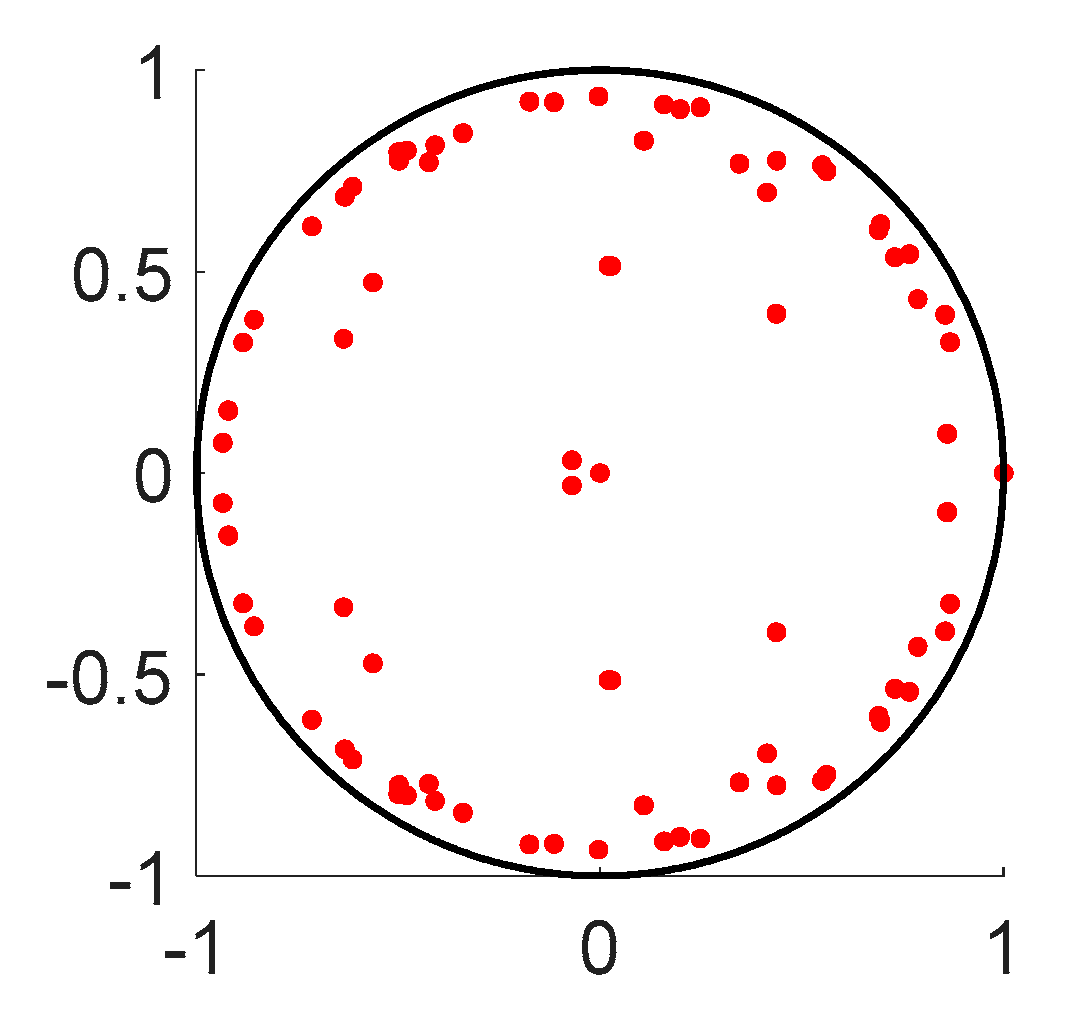
We consider the 2-D case in the following analysis. The preselected integer N is selected as 20, and $l=2^{20}$ in the proposed method. The natural angular frequency of the magnetized plasma discussed is $2\pi \times 28.7\times {10}^9 \mathrm{rad}/\mathrm{s}$, the collision frequency is 20 GHz, and the electron cyclotron frequency is set as $1.0\times {10}^{11} \mathrm{rad}/\mathrm{s}$. Figure 3 graphs the comparison of the unit circle and the eigenvalues of the exponential matrix T in the complex plane when the time-step size is ${10}^6\Delta t_{\mathrm{CFL}}$. Here, $\Delta t_{\mathrm{CFL}}$ is the upper limit time-step size of the conventional FDTD method. It is clear seen that all the eigenvalues are within or on the unit circle, which means that the presented PITD method of the magnetized plasma is stable under such a large time-step size. Therefore, the proposed formulation can use a time-step size much larger than the maximum value of the CFL stability condition to achieve the simulation of the magnetized plasma problems.

3.2. Numerical Dispersion Analysis

In this subsection, the dispersion performance of the presented PITD method in magnetized plasma is discussed numerically by adopting the Fourier approach. The dispersion performance of the presented formulation is described by the differences between the numerical wave number k_num and the analytical wave number k_anal. Suppose c is the velocity of light in the vacuum, the analytic wave number of the left-hand circularly polarized (LCP) EM wave is:

$$k_L=\frac{\omega }{c}\sqrt{1-\frac{{\omega }_p^2}{{\omega }^2\left[\left(1-j\frac{\gamma }{\omega }\right)+\frac{{\omega }_b}{\omega }\right]}},$$

(17)

and the analytic wave number of the right-hand circularly polarized (RCP) EM waves is:

$$k_R=\frac{\omega }{c}\sqrt{1-\frac{{\omega }_p^2}{{\omega }^2\left[\left(1-j\frac{\gamma }{\omega }\right)-\frac{{\omega }_b}{\omega }\right]}}.$$

(18)

Assuming that the monochromatic plane wave propagates in the magnetized plasma, the field components are expressed as:

$$X=X_0{e}^{-j(kz-\omega t)},$$

(19)

where k is the wave number, X₀ and ω are the amplitude and the angular frequency of the EM wave, respectively. The discrete form of Equation (19) is obtained as follows:

$$X_k=X_0{e}^{-j(km\Delta z-\omega n\Delta t)},$$

(20)

where m and n are the space index and the time index, respectively.

Here, we consider the 1-D case, and the vector X includes the field components E_x, E_y, H_x, H_y, J_x, and J_y. Substituting the discrete form of the field components into Equation (2) for the 1-D case, a homogenous system of ODEs can be obtained and written in matrix form as:

$$\frac{\mathrm{d}X}{\mathrm{d}t}=H_{1}X.$$

(21)

Here, the coefficient matrix H₁ is:

$$H_1=\left[\begin{array}{cccccc}0& 0& 0& \frac{jW}{{\epsilon }_0}& -\frac{1}{{\epsilon }_0}& 0\\ 0& 0& -\frac{jW}{{\epsilon }_0}& 0& 0& -\frac{1}{{\epsilon }_0}\\ 0& -\frac{jW}{{\mu }_0}& 0& 0& 0& 0\\ \frac{jW}{{\mu }_0}& 0& 0& 0& 0& 0\\ {\epsilon }_0{\omega }_p^2& 0& 0& 0& -\gamma & -{\omega }_b\\ 0& {\epsilon }_0{\omega }_p^2& 0& 0& {\omega }_b& -\gamma \end{array}\right],$$

(22)

where:

$$W=\frac{2\sin \left(\frac{1}{2}k\Delta z\right)}{\Delta z}.$$

(23)

The following discrete iterative formula is used to solve the ODEs Equation (21):

$$X_{k+1}=T_1{X}_k,$$

(24)

where the exponential matrix T₁ is:

$$T_1={\left[I+\left(H_{1}s\right)+\frac{{\left(H_{1}s\right)}^2}{2!}+\frac{{\left(H_{2}s\right)}^3}{3!}+\frac{{\left(H_{3}s\right)}^4}{4!}\right]}^l.$$

(25)

Then, we have:

$$\left(e^{j\omega t}I-T_1\right)X_0=0.$$

(26)

Since it is true for any X₀ that is nonzero, the determinant of the coefficient matrix $\left(e^{j\omega t}I-T\right)$ should be zero:

$$\left(e^{j\omega t}I-T_1\right)=0.$$

(27)

In the following analysis, the numerical dispersion error and the numerical dissipation error are defined to describe the precision of the presented PITD method in the magnetized plasma. The definition of the relative dispersion error is (Re(k_num)−Re(k_anal))/Re(k_anal), and it is related to the phase error. The definition of the relative dissipation error is (Im(k_num)−Im(k_anal))/Im(k_anal), and it is related to the amplitude error [27].

It is assumed that $\Delta z=75 \mathsf{\mu }\mathrm{m}$, $\Delta t=0.125 \mathrm{ps}$, and ${\omega }_b=3.0\times {10}^{11} \mathrm{rad}/\mathrm{s}$. The preselected integer N is chosen as 20, and $l=2^{20}$ in the presented PITD method. The solutions of numerical wave number are computed by Equation (27).

3.2.1. Effect of Wave Frequency on Numerical Error

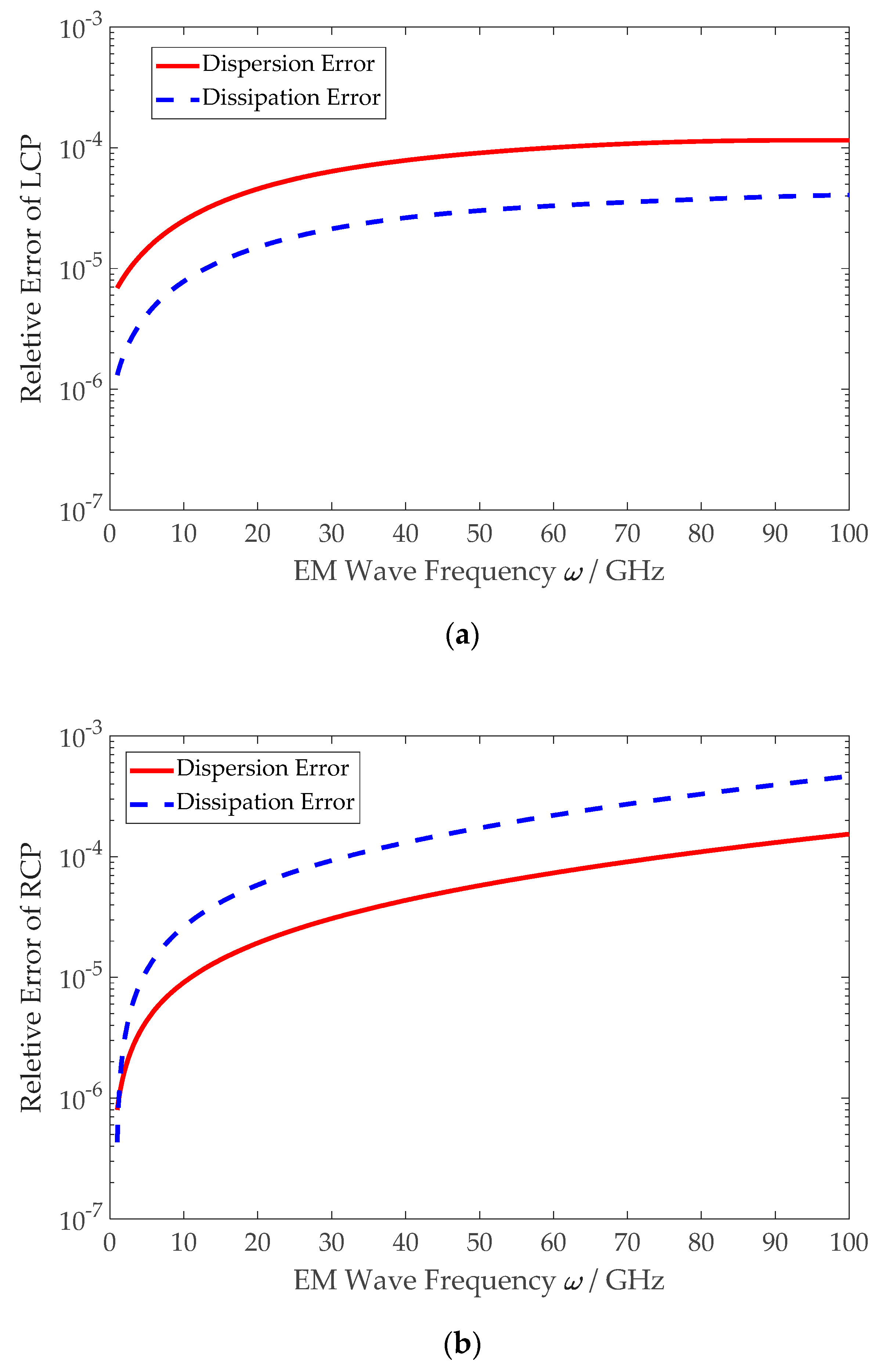
The natural angular frequency of the magnetized plasma is ${\omega }_p=2\pi \times 50\times {10}^9 \mathrm{rad}/\mathrm{s}$. The collision frequency is 20 GHz. Figure 4a,b graphs the relative dispersion and relative dissipation errors with respect to the wave frequency ω for both the LCP and RCP waves, respectively. We can see that both the dispersion and dissipation errors increase monotonically with the wave frequency. Furthermore, the relative dispersion error is higher than the relative dissipation error in the LCP wave, and is lower than the relative dissipation error in the RCP wave. In addition, the relative error range of the proposed PITD method is ${10}^{-6}$ to $5\times {10}^{-4}$ when the EM wave frequency is from 1 GHz to 100 GHz.

3.2.2. Effect of the Natural Angular Frequency on Numerical Error

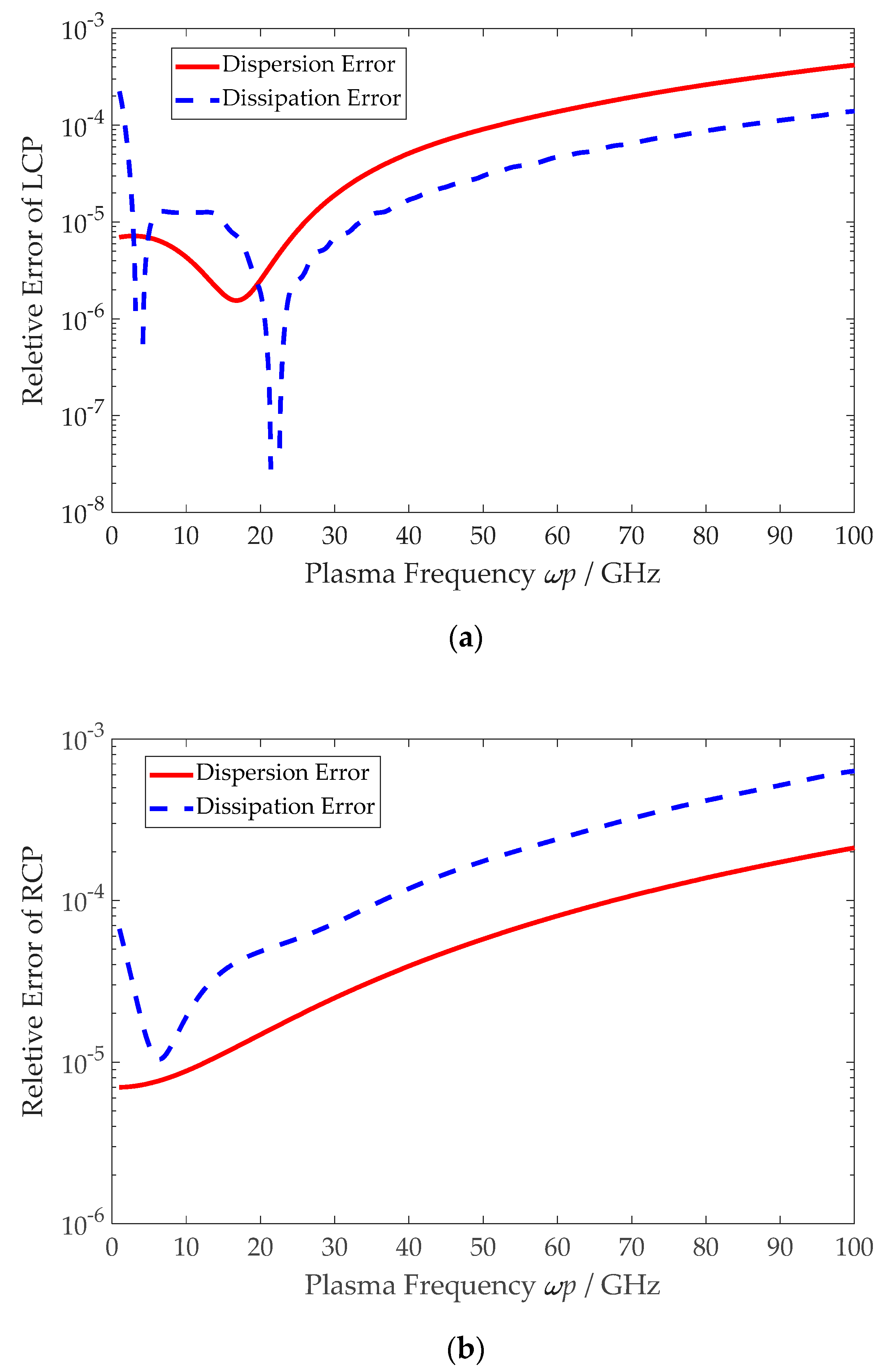
The EM wave frequency is set as 50 GHz. The collision frequency of the magnetized plasma is 20 GHz. Figure 5a,b graphs the relative dispersion and relative dissipation errors with respect to the natural angular frequency ω_p for both the LCP and RCP waves, respectively. For the LCP wave, the relative dispersion error curve has lower-peak error when ω_p/2π is 18 GHz, and the relative dissipation error curve has lower-peak errors when ω_p/2π are 4 GHz and 21 GHz. For the RCP wave, the relative dispersion error curve has no lower-error peak, and the relative dissipation error curve has lower-peak error when ω_p/2π is 6 GHz. Moreover, both the relative dispersion and relative dissipation errors increase monotonically with the natural frequency when ω_p/2π is larger than the frequency of the lower-peak error.

3.2.3. Effect of the Plasma Collision Frequency on Numerical Error

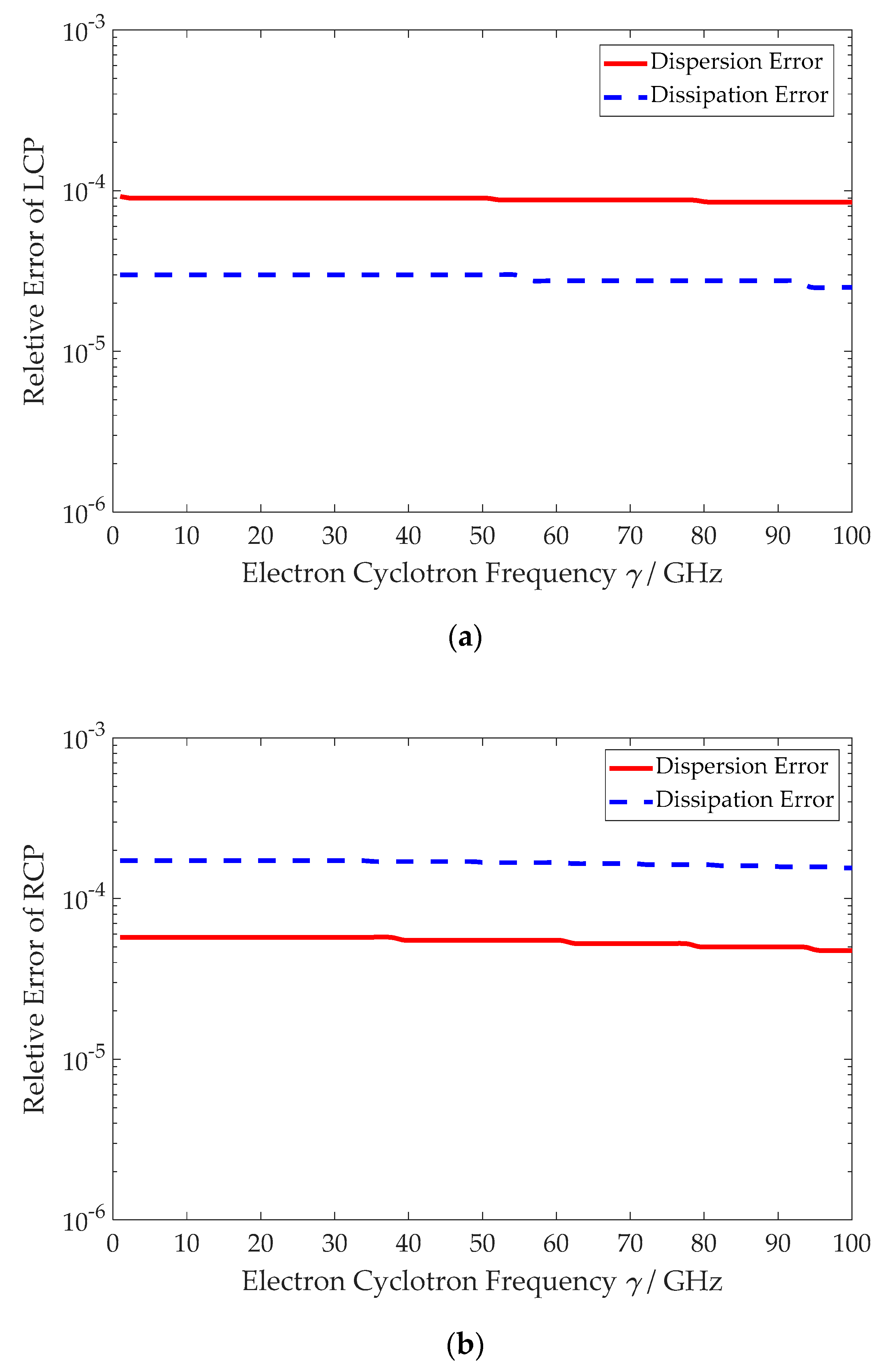
The EM wave frequency is set as 50 GHz, and the natural angular frequency is ${\omega }_p=2\pi \times 50\times {10}^9 \mathrm{rad}/\mathrm{s}$. Figure 6a,b graphs the relative dispersion and relative dissipation errors with respect to the collision frequency γ for both the LCP and RCP waves, respectively. It is found that the relative dispersion and relative dissipation errors are slightly decreased when the collision frequency is increased.

3.2.4. Effect of the Time-Step Size on Numerical Error

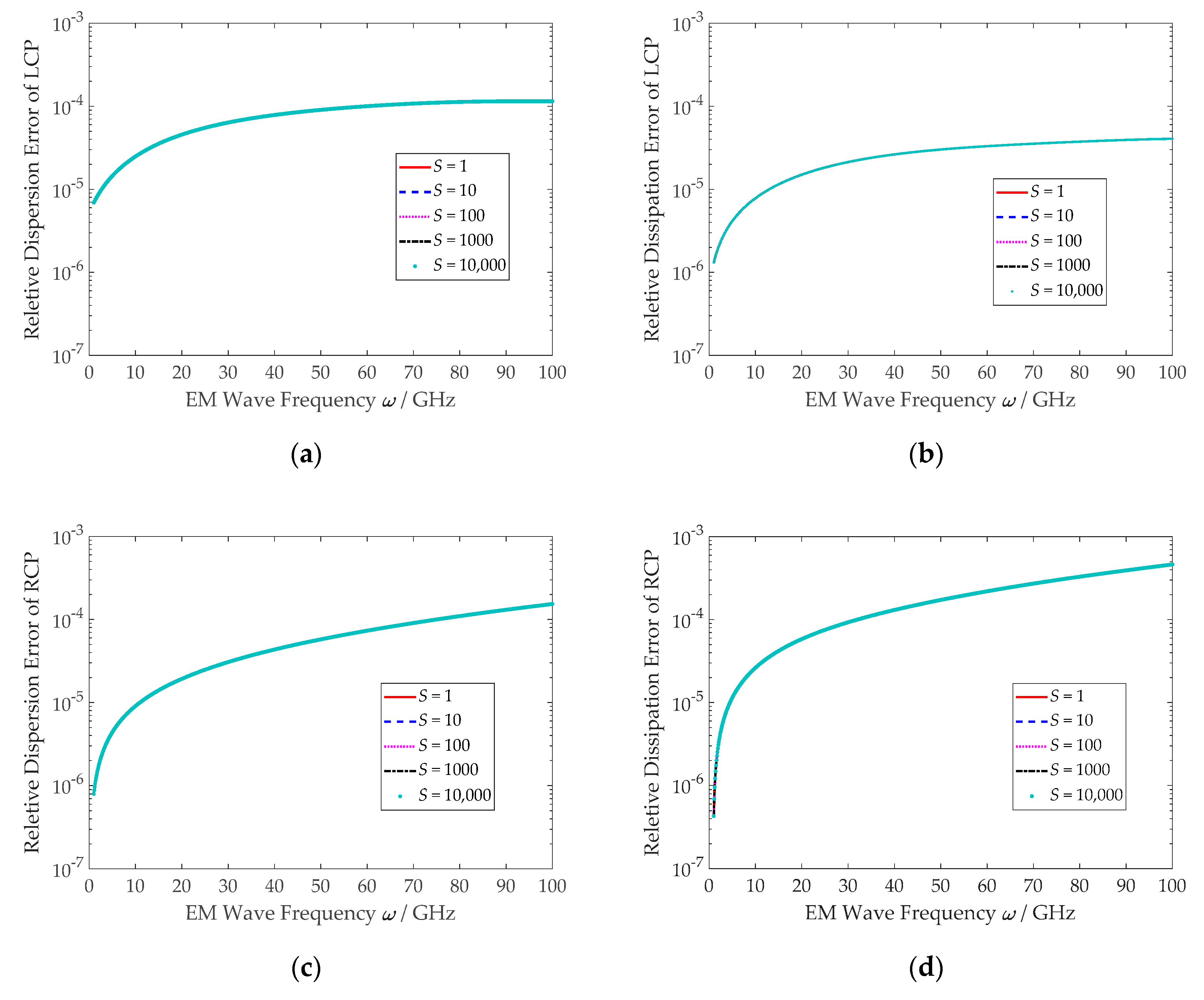
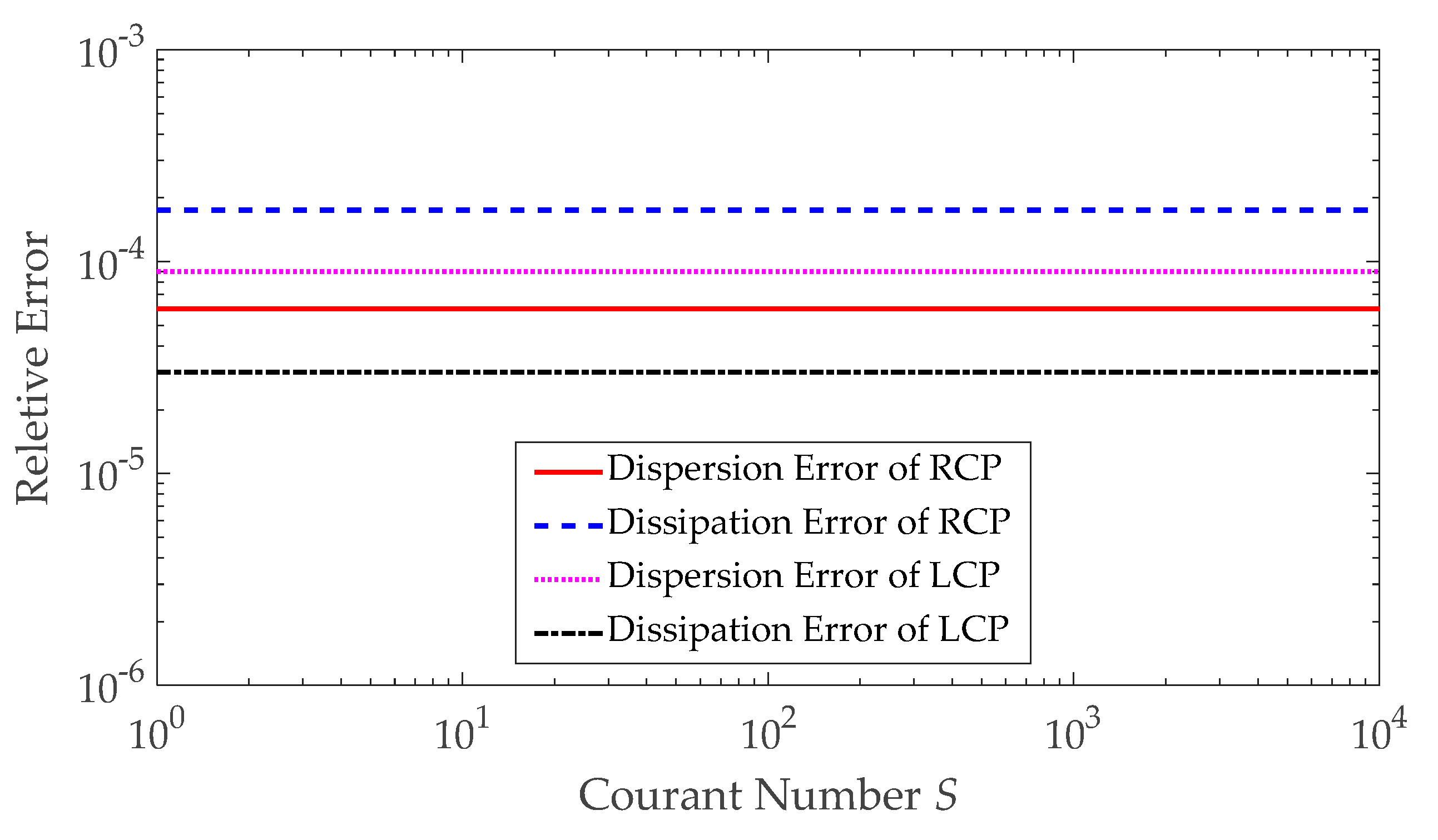
It is assumed that the natural angular frequency is $2\pi \times 50\times {10}^9 \mathrm{rad}/\mathrm{s}$, and the collision frequency is 20 GHz. Figure 7 graphs the relative dispersion and relative dissipation errors with respect to the wave frequency ω for both the LCP and RCP waves under different Courant number S, respectively. It is clear that all the curves are in agreement. Figure 8 shows the relative dispersion and relative dissipation errors with respect to the Courant number when the EM wave frequency is 50 GHz. Figure 8 indicates that the relative dispersion and relative dissipation errors are almost invariant when the Courant numbers is increased. These mean that the proposed method can maintain a lower numerical dispersion error in the simulations when the time step is increased.

4. Numerical Experiments

The performance of the presented PITD method are verified by two typical magnetized plasma examples which are also solved by the analytical formulas and the formulations based on the FDTD method, respectively, for comparison.

4.1. Magnetized Plasma Slab

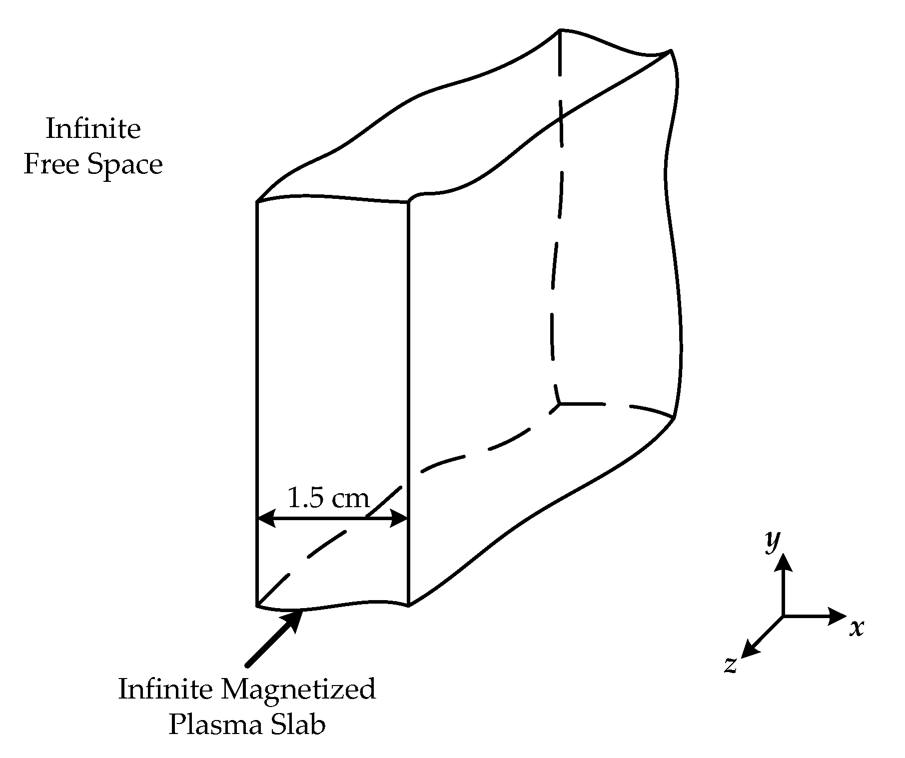
As the first example, a magnetized plasma slab is simulated to validate the efficiency and the accuracy of the modified PITD algorithm in this paper. The diagram of the infinite magnetized plasma slab in infinite free space is shown in Figure 9. The numerical reflection coefficient and transmission coefficient are computed by the presented method, the JEC-FDTD method and the ADE-FDTD method, respectively. The results are also compared with the analytical solution.

The magnetized plasma slab is 1.5 cm thick, and divided into 200 cells, i.e., the space step is $75 \mathsf{\mu }\mathrm{m}$. The main computing region is composed of 600 free space cells (the space indexes are from 1 to 300, and 501 to 800) and 200 magnetized plasma cells (the space indexes are from 301 to 500). Perfectly matched layer (PML) is employed as the absorption boundary condition to eliminate the reflection error. The time-step size of the methods based on the FDTD formulation is set to $\Delta t_{\mathrm{FDTD}}=0.125 \mathrm{ps}$, and the time-step size of the proposed PITD method is 5 times of $\Delta t_{\mathrm{FDTD}}$ (i.e., $\Delta t_{\mathrm{Proposed}\mathrm{PITD}}=0.625 \mathrm{ps}$). The parameters of the magnetized plasma are shown as follows:

$${\omega }_p=2\pi \times 28.7\times {10}^9\mathrm{rad}/\mathrm{s},$$

(28)

$$\gamma =20.0 \mathrm{GHz},$$

(29)

$${\omega }_b=1.0\times {10}^{11} \mathrm{rad}/\mathrm{s}.$$

(30)

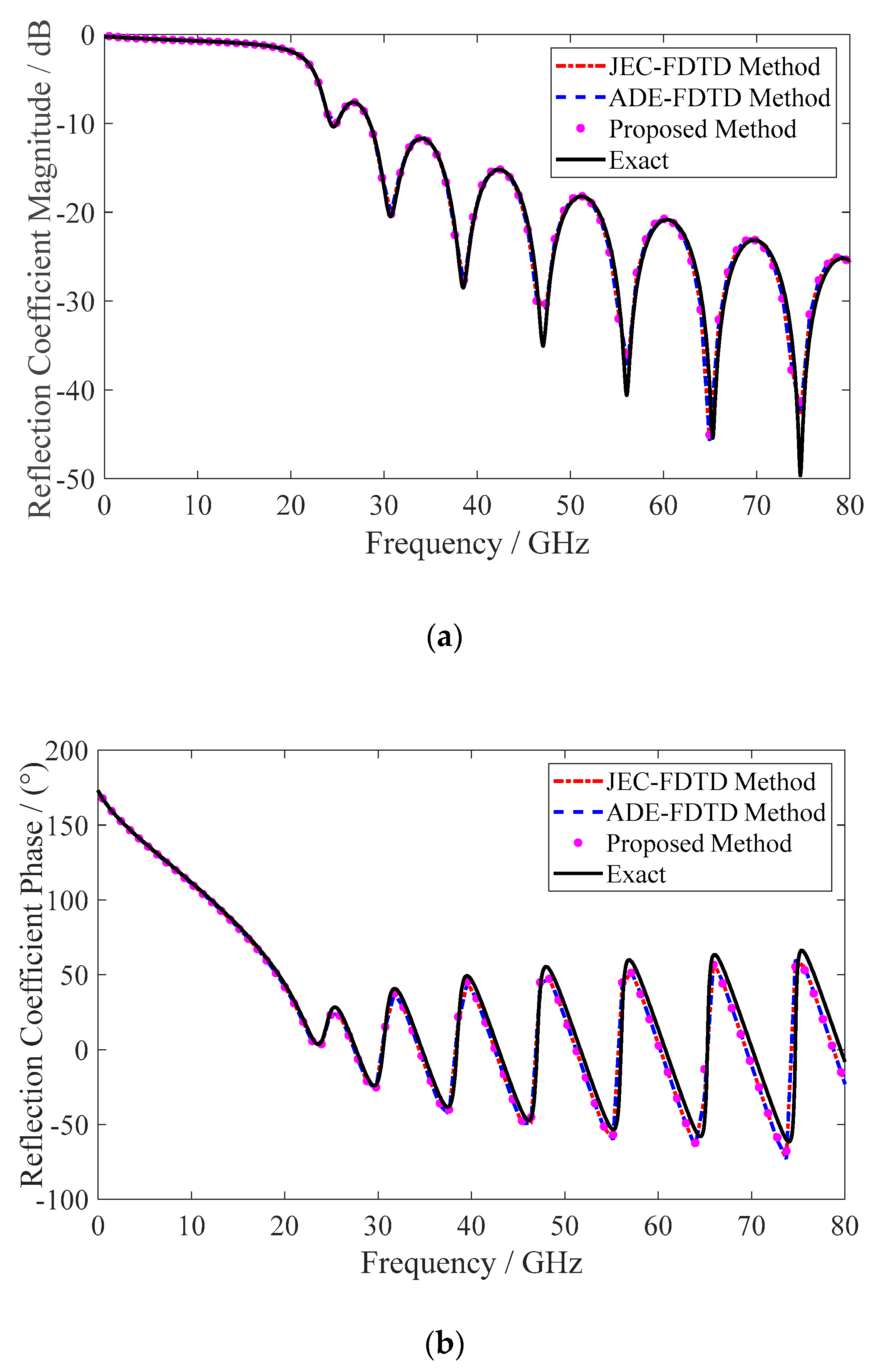
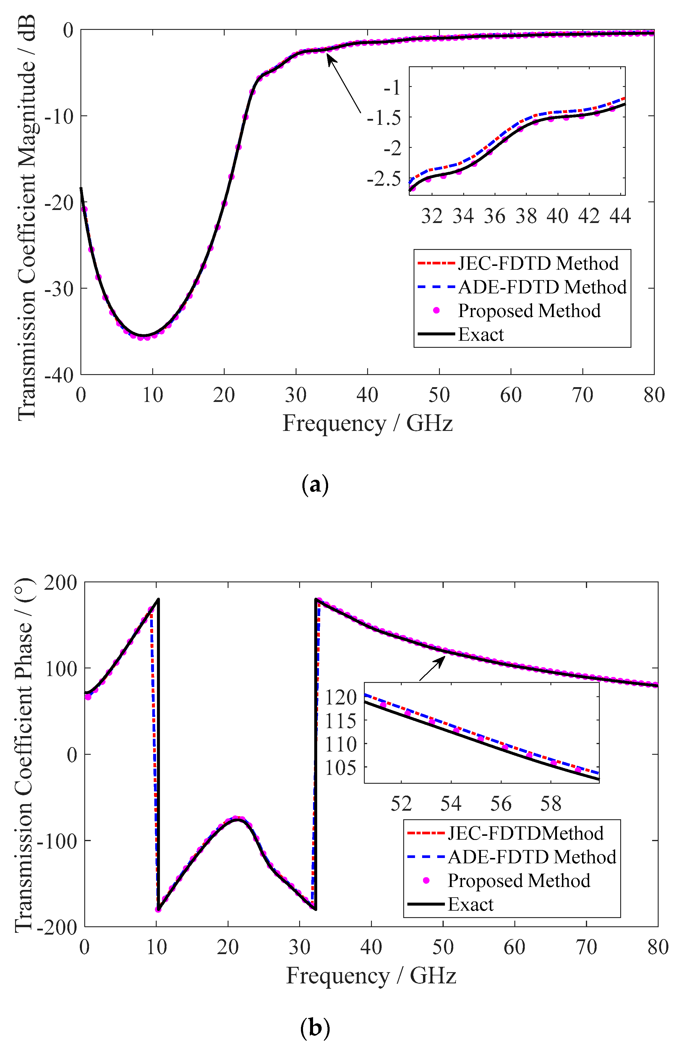
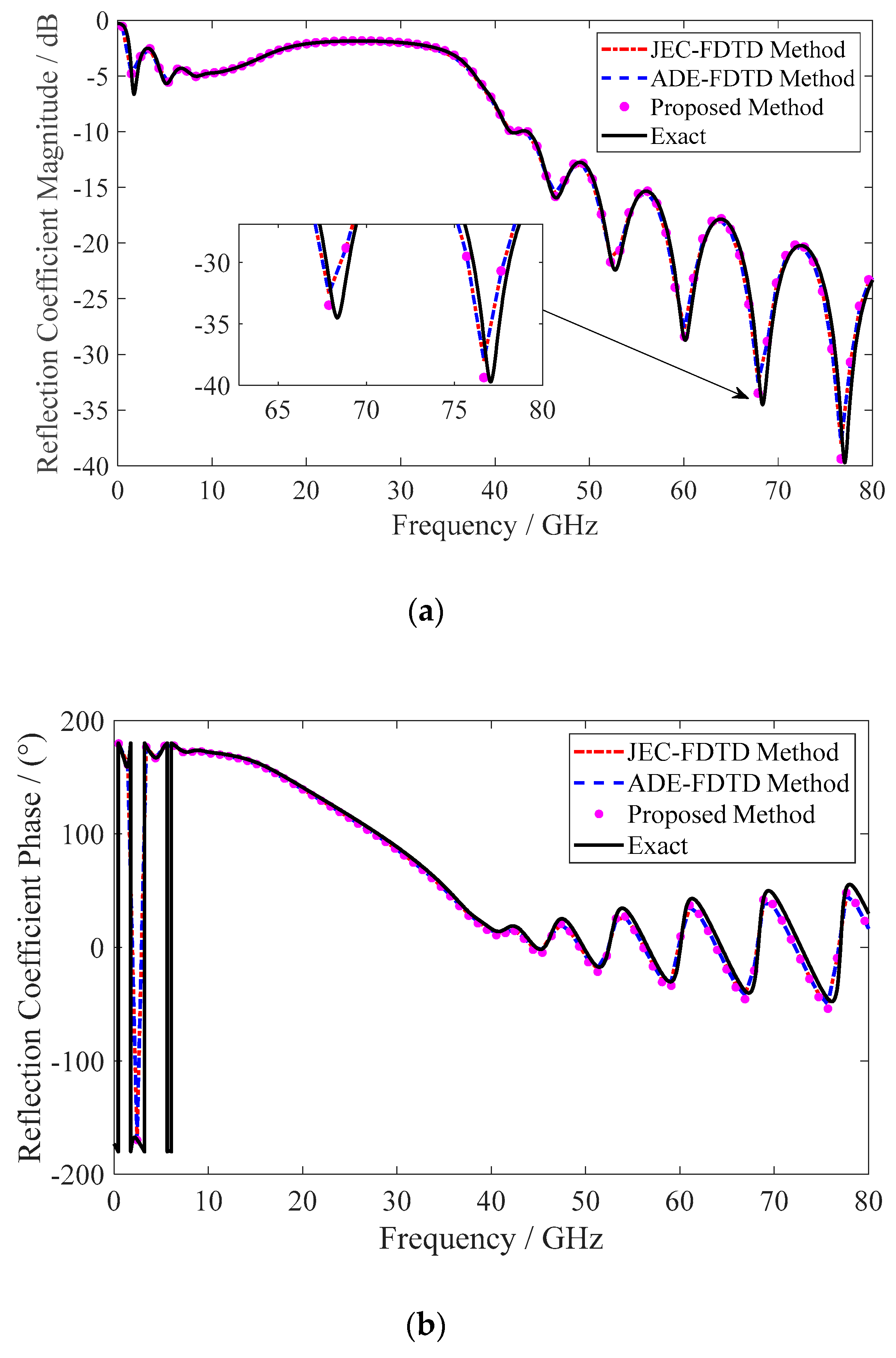
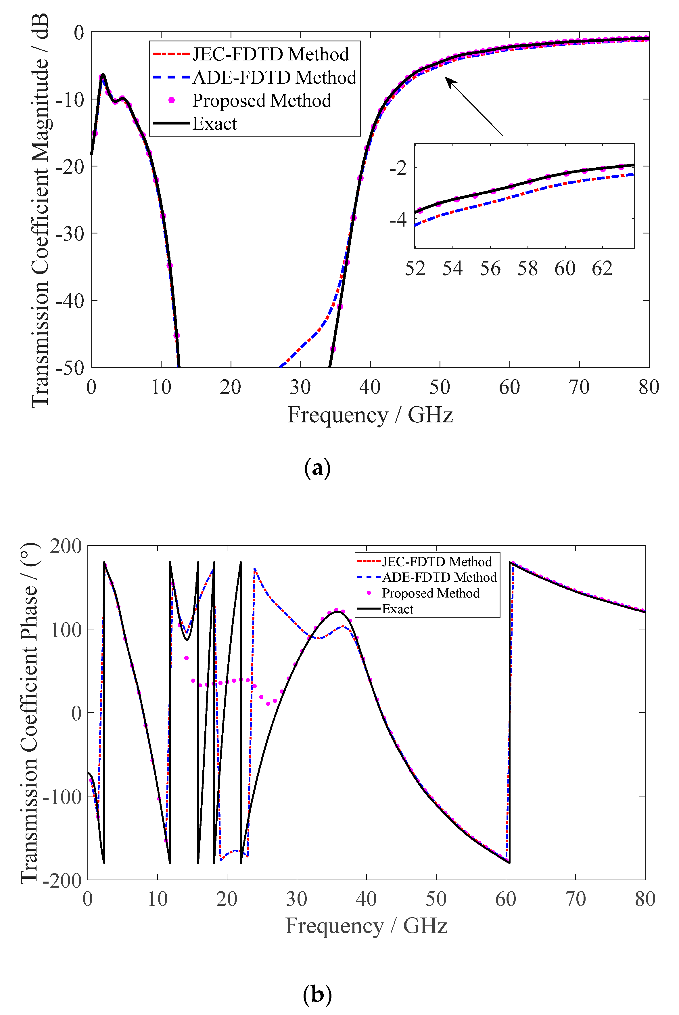
Figure 10, Figure 11, Figure 12 and Figure 13 show the magnitude and the phase of the complex reflection coefficient and transmission coefficient of the magnetized plasma slab calculated by the JEC-FDTD method, the ADE-FDTD method, the proposed PITD method, and the analytical solution, respectively. We can clearly see that the computational results of the proposed PITD method are coincident with the analytical solutions on both the magnitude and the phase.

According to Figure 11, Figure 12a and Figure 13, it should be noted that the solutions of the proposed PITD method is more accurate than those of the JEC-FDTD method and the ADE-FDTD method, especially in the higher frequency range. Meanwhile, it is also found that larger errors occur in the stopband of the transmission coefficient for the RCP wave. Figure 13 shows that larger errors occur from 13 GHz to 38 GHz for the FDTD methods, and from 13 GHz to 27 GHz for the proposed method. This means that the low computational error range of the presented PITD method is larger than the FDTD methods.

The CPU time of the three methods are also recorded. The execution time of the JEC-FDTD method, the ADE-FDTD method, and the presented method are 8.50 s, 8.09 s, and 4.52 s, respectively. It can be concluded that a larger simulated time step leads to an appreciably reduction of the CPU time.

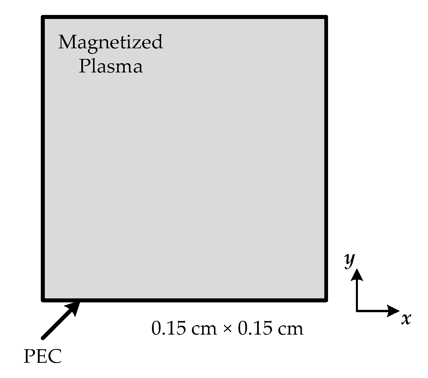
4.2. 2-D Magnetized Plasma Filled Cavity

The second example is a 2-D cavity filled with the magnetized plasma as shown in Figure 14. The main computing region is divided into 20 × 20 cells with a space step $75 \mathsf{\mu }\mathrm{m}$. The time-step size of the ADE-FDTD method is $\Delta t=0.1 \mathrm{ps}$. For the proposed PITD method, the time-step size is $6\Delta t$ in this example. Therefore, the simulations are executed by 3000 iterative steps in the ADE-FDTD method and 500 iterative steps in the presented PITD method. The parameters of the magnetized plasma filled in the cavity are ${\omega }_p=2\pi \times 28.7\times {10}^9 \mathrm{rad}/\mathrm{s}$, $\gamma =10.0 \mathrm{GHz}$, and ${\omega }_b=3.0\times {10}^{11} \mathrm{rad}/\mathrm{s}$.

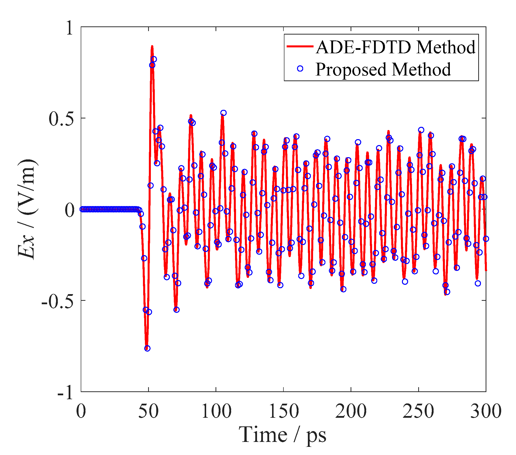
Figure 15 graphs the time-domain waveforms of the electric field E_x simulated by the presented PITD method and the ADE-FDTD method, respectively. It is shown that good agreements are achieved between the two methods on the simulated waveform.

Table 1. A comparison of calculated frequencies and execution time between the auxiliary differential equation finite-difference time-domain (ADE-FDTD) method and the proposed precise-integration time-domain (PITD) method.

Method	Resonant Frequency/GHz			Execution Time/s
ADE-FDTD	30.76	103.5	201.7	12.85
Proposed PITD	31.25	103.5	201.2	8.07

lists the numerical resonant frequencies and the execution time of the presented PITD method and the ADE-FDTD method, respectively. It can be found that the calculated resonant frequencies are also coincident, moreover, the CPU time of the presented method is at least 1/3 less than that of the ADE-FDTD method. The simulations of both the FDTD methods and the PITD method in above analysis are achieved by MATLAB and performed on Intel(R) Core(TM) i3 CPU M370 2.40 GHz PC (Intel, Santa Clara, CA, USA).

In conclusion, according to the numerical experiments above, the efficiency of the modified PITD method in this paper is higher than the algorithms based on the FDTD scheme for modeling the magnetized plasma. Meanwhile, the solutions of the magnetized plasma slab validate that the presented method is more accurate than the JEC-FDTD method and the ADE-FDTD method, especially in the high frequency range.

5. Conclusions

Based on both the auxiliary differential equation and the PI technique, a modified PITD method has been proposed for modeling the EM wave propagation through magnetized plasma in this paper. The analyses of the numerical stability and dispersion are discussed respectively, and the superior performance of the proposed method has been confirmed numerically. It is found that the numerical stability criterion of the proposed method is much looser than the CFL stability condition of the FDTD methods so as to increase the allowable simulated time step, and the numerical dispersion error and the dissipation error are almost invariant when the time step is increased. The numerical results validate the efficiency and accuracy of the presented algorithm. In the numerical experiments above, the proposed method can use a time-step size much larger than the value allowed by the CFL limit of the FDTD method which leads to a reduction of the CPU time in the simulation. Meanwhile, the accuracy performance of the presented PITD method is better than the JEC-FDTD method and the ADE-FDTD method, especially in higher frequency range. In conclusion, the proposed algorithm is a strong numerical tool to solve the EM wave problems in the magnetized plasma.

References

- Letsholathebe, D.; Mphale, K. Microwave phase perturbation and ionisation measurement in vegetation fire plasma. IET Microw. Antennas Propag. 2013, 7, 741–745. [Google Scholar] [CrossRef]
- Nadal, C.; Pigache, F.; Lefevre, Y. First approach for the modelling of the electric field surrounding a piezoelectric transformer in view of plasma generation. IEEE Trans. Magn. 2012, 48, 423–426. [Google Scholar] [CrossRef] [Green Version]
- Li, X.S.; Hu, B.J. FDTD Analysis of a magneto-plasma antenna with uniform or nonuniform distribution. IEEE Antennas Wirel. Propag. Lett. 2010, 9, 175–178. [Google Scholar] [CrossRef]
- Chai, S.W.; Lim, S.M.; Hong, S.C. THz detector with an antenna coupled stacked CMOS plasma-wave FET. IEEE Microw. Wirel. Compon. Lett. 2014, 24, 869–871. [Google Scholar] [CrossRef]
- Vyas, H.; Chaudhury, B. Computational investigation of power efficient plasma-based reconfigurable microstrip antenna. IET Microw. Antennas Propag. 2018, 12, 1587–1593. [Google Scholar] [CrossRef]
- Krishna, T.N.V.; Sathishkumar, P.; Himasree, P.; Punnoose, D.; Raghavendra, K.V.G.; Naresh, B.; Rana, R.A.; Kim, H.J. 4T analog MOS control-high voltage high frequency (HVHF) plasma switching power supply for water purification in industrial applications. Electronics 2018, 7, 245. [Google Scholar] [CrossRef] [Green Version]
- Liu, J.F.; Lv, H.; Zhao, Y.C.; Fang, Y.; Xi, X.L. Stochastic PLRC-FDTD method for modeling wave propagation in unmagnetized plasma. IEEE Antennas Wirel. Propag. Lett. 2018, 17, 1024–1028. [Google Scholar] [CrossRef]
- Shibayama, J.; Takahashi, R.; Yamauchi, J.; Nakano, H. Frequency-dependent LOD-FDTD implementations for dispersive media. Electron. Lett. 2006, 42, 1084–1086. [Google Scholar] [CrossRef]
- Ramadan, O. Stability-improved ADE-FDTD implementation of Drude dispersive models. IEEE Antennas Wirel. Propag. Lett. 2018, 17, 877–880. [Google Scholar] [CrossRef]
- Ramadan, O. Efficient ADE-WE-PML formulations for scalar dispersive FDTD applications. Electron. Lett. 2013, 49, 157–158. [Google Scholar] [CrossRef]
- Li, J.X.; Wu, P.Y.; Jiang, H.L. Implementation of higher order CNAD CFS-PML for truncating unmagnetised plasma. IET Microw. Antennas Propag. 2019, 13, 756–760. [Google Scholar] [CrossRef]
- Li, J.; Dai, J. Z-Transform implementations of the CFS-PML. IEEE Antennas Wirel. Propag. Lett. 2006, 5, 410–413. [Google Scholar] [CrossRef]
- Taflove, A.; Hagness, S.C. Computational Electrodynamics: The Finite-Difference Time-Domain Method; Artech House: Boston, MA, USA, 2005. [Google Scholar]
- Namiki, T. A new FDTD algorithm based on alternating-direction implicit method. IEEE Trans. Microw. Theory Tech. 1999, 47, 2003–2007. [Google Scholar] [CrossRef]
- Namiki, T. 3-D ADI-FDTD method-unconditionally stable time-domain algorithm for solving full vector Maxwell’s equations. IEEE Trans. Microw. Theory Tech. 2000, 48, 1743–1748. [Google Scholar] [CrossRef]
- Shibayama, J.; Muraki, M.; Yamauchi, J.; Nakano, H. Efficient implicit FDTD algorithm based on locally one-dimensional scheme. Electron. Lett. 2005, 41, 1046–1047. [Google Scholar] [CrossRef]
- Ahmed, I.; Chua, E.K.; Li, E.P.; Chen, Z. Development of the three-dimensional unconditionally stable LOD-FDTD method. IEEE Trans. Antennas Propag. 2008, 56, 3596–3600. [Google Scholar] [CrossRef]
- Liang, T.L.; Shao, W.; Shi, S.B.; Ou, H. Analysis of extraordinary optical transmission with periodic metallic gratings using ADE-LOD-FDTD method. IEEE Photonics J. 2016, 8, 7804710. [Google Scholar] [CrossRef]
- Ma, X.K.; Zhao, X.T.; Zhao, Y.Z. A 3-D precise integration time-domain method without the restrains of the Courant-Friedrich-Levy stability condition for the numerical solution of Maxwell’s equations. IEEE Trans. Microw. Theory Tech. 2006, 54, 3026–3037. [Google Scholar]
- Song, W.J.; Zhang, H. RKADE-ADI FDTD applied to analysis of terahertz wave characteristics of plasma. IET Microw. Antennas Propag. 2017, 11, 1071–1077. [Google Scholar]
- Liang, T.L.; Shao, W.; Shi, S.B. Complex-envelope ADE-LOD-FDTD for band gap analysis of plasma photonic crystals. Appl. Comput. Electromagn. Soc. J. 2018, 33, 443–449. [Google Scholar]
- Sun, G.; Ma, X.K.; Bai, Z.M. Numerical stability and dispersion analysis of the precise-integration time-domain method in lossy media. IEEE Trans. Microw. Theory Tech. 2012, 60, 2723–2729. [Google Scholar] [CrossRef]
- Kang, Z.; Li, W.L.; Wang, Y.F.; Huang, M.; Yang, F. A precise-integration time-domain formulation based on auxiliary differential equation for transient propagation in plasma. IEEE Access 2020, 8, 59741–59749. [Google Scholar] [CrossRef]
- Jiang, L.L.; Chen, Z.Z.; Mao, J.F. On the numerical stability of the precise integration time-domain (PITD) method. IEEE Microw. Wirel. Compon. Lett. 2007, 17, 471–473. [Google Scholar] [CrossRef]
- Kang, Z.; Ma, X.K.; Zhuansun, X. An efficient 2-D compact precise-integration time-domain method for longitudinally invariant waveguiding structures. IEEE Trans. Microw. Theory Tech. 2013, 61, 2535–2544. [Google Scholar] [CrossRef]
- Bai, Z.M.; Ma, X.K.; Sun, G. A low-dispersion realization of precise integration time-domain method using a fourth-order accurate finite difference scheme. IEEE Trans. Antennas Propag. 2011, 59, 1311–1320. [Google Scholar] [CrossRef]
- Zhong, S.Y.; Lai, Z.Q.; Liu, S.; Liu, S.B. The numerical dispersion relation and stability analysis of PLCDRC-FDTD method for anisotropic magnetized plasma. In Proceedings of the International Conference on Microwave and Millimeter Wave Technology, Nanjing, China, 21–24 April 2008. [Google Scholar]
Figure 1.
Numerical velocity of the finite-difference time-domain (FDTD), precise-integration time-domain (PITD) and alternating-direction implicit FDTD (ADI-FDTD) methods versus the propagation angle when the Courant number is S = 0.5.
Figure 2.
Numerical velocity of the PITD and ADI-FDTD methods versus the propagation angle under different Courant numbers.
Figure 3.
Comparison of the unit circle and the eigenvalues of the presented PITD algorithm in the complex plane.
Figure 4.
Relative dispersion and relative dissipation errors with respect to the electromagnetic (EM) wave frequency: (a) The left-hand circularly polarized (LCP) wave. (b) The right-hand circularly polarized (RCP) wave.
Figure 5.
Relative dispersion and relative dissipation errors with respect to the natural frequency: (a) The LCP wave. (b) The RCP wave.
Figure 6.
Relative dispersion and relative dissipation errors with respect to the collision frequency: (a) The LCP wave. (b) The RCP wave.
Figure 7.
Relative dispersion and relative dissipation errors with respect to the wave frequency under different Courant numbers: (a) Relative dispersion error of the LCP wave. (b) Relative dissipation error of the LCP wave. (c) Relative dispersion error of the RCP wave. (d) Relative dissipation error of the RCP wave.
Figure 8.
Relative dispersion and relative dissipation errors with respect to the Courant numbers for the LCP wave and the RCP wave.
Figure 9.
The diagram of the magnetized plasma slab in free space.
Figure 10.
Calculated complex reflection coefficient of the LCP wave: (a) Magnitude. (b) Phase.
Figure 11.
Calculated complex transmission coefficient of the LCP wave: (a) Magnitude. (b) Phase.
Figure 12.
Calculated complex reflection coefficient of the RCP wave: (a) Magnitude. (b) Phase.
Figure 13.
Calculated complex transmission coefficient of the RCP wave: (a) Magnitude. (b) Phase.
Figure 14.
The diagram of the 2-D cavity filled with the magnetized plasma.
Figure 15.
The time-domain waveforms of the electric field Ex simulated by the proposed PITD method and the auxiliary differential equation FDTD (ADE-FDTD) method.