Real-Time Collision-Free Navigation of Multiple UAVs Based on Bounding Boxes


Computing Systems Department, Universidad de Castilla–La Mancha (UCLM), Campus Universitario, s/n, 02071 Albacete, Spain
*
Author to whom correspondence should be addressed.
Electronics 2020, 9(10), 1632; https://0-doi-org.brum.beds.ac.uk/10.3390/electronics9101632
Submission received: 2 September 2020
/
Revised: 28 September 2020
/
Accepted: 30 September 2020
/
Published: 3 October 2020
(This article belongs to the Special Issue Autonomous Navigation Systems: Design, Control and Applications)
Abstract
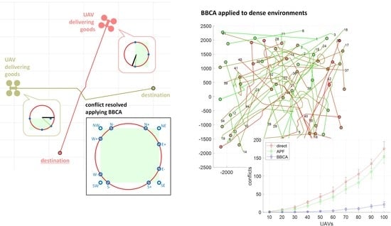
:Predictably, future urban airspaces will be crowded with autonomous unmanned aerial vehicles (UAVs) offering different services to the population. One of the main challenges in this new scenario is the design of collision-free navigation algorithms to avoid conflicts between flying UAVs. The most appropriate collision avoidance strategies for this scenario are non-centralized ones that are dynamically executed (in real time). Existing collision avoidance methods usually entail a high computational cost. In this work, we present Bounding Box Collision Avoidance (BBCA) algorithm, a simplified velocity obstacle-based technique that achieves a balance between efficiency and cost. The performance of the proposal is analyzed in detail in different airspace configurations. Simulation results show that the method is able to avoid all the conflicts in two UAV scenarios and most of them in multi-UAV ones. At the same time, we have found that the penalty of using the BBCA collision avoidance technique on the flying time and the distance covered by the UAVs involved in the conflict is reasonably acceptable. Therefore, we consider that BBCA may be an excellent candidate for the design of collision-free navigation algorithms for UAVs.
1. Introduction
In the not-too-distant future, unmanned aerial vehicles (UAVs) will be a common element in airspace. Their use in recent years has increased exponentially, and this is mainly due to cost savings, their autonomy, and consequently the absence of risk from the human factor. Technological advances such as navigation, dynamics, sensors, and communications make it possible to use them for different applications—not only military but also civilian uses. Among the services offered by these UAVs are the delivery of parcels, precision agriculture, fire detection and fighting, maritime surveillance, transport of medical equipment, etc.
Although the growth in the use of UAVs in civil applications is relatively new, guidelines or requirements have already been developed to regulate the use of these vehicles in airspace. However, it should be added that there is no global regulation and depending on each country there are a number of restrictions such as weather conditions, maximum and minimum flight height, prohibited flight zones, and compulsory use of onboard “Sense and Avoid” systems.
The increase in the use of these vehicles for various applications has made the scientific community not only focus on their aerodynamics or the materials or chipsets of which they are composed, but a new challenge arises that is of greater interest—the design of collision-free path/trajectory planning mechanisms, especially in future crowded airspaces [1]. Therefore, a prerequisite arises for these multi-UAV systems to be able to succeed in the new applications they face—the ability to avoid collision. This capacity must be incorporated to comply with the regulations concerning autonomous UAVs.
In likely future scenarios, with hundreds or thousands of UAVs offering different types of services and sharing the same airspace, it is not feasible to develop a centralized path planning strategy that ensures the absence of collisions between all these UAVs. Therefore, a decentralized (or coordinated) collision avoidance strategy must be put in place, so that UAVs can dynamically detect and resolve these situations.
This paper therefore focuses on real-time collision avoidance in multi-UAV systems. As a starting point, it should be added that there are a number of characteristics that make the resolution of this problem complex: obstacles are dynamic and their velocity and direction may dynamically vary, entities using real-time decision-making and information with consequent delays, etc.
Existing collision avoidance proposals include, among others, the use of potential field methods, evolutionary algorithms, graph-based techniques, search in the state space, geometric relations, forces, or velocities. In this work we propose a decentralized mechanism that slightly modifies the route followed by the UAVs involved in the conflict. The mechanism uses a box delimitation algorithm according to the well-known velocity obstacle method. The use of this strategy significantly reduces the algorithmic complexity and computational cost of traditional proposals. At the same time, as we will see, its efficiency is high.
The rest of this work is structured as follows. Next, Section 2 presents a general taxonomy of collision avoidance mechanisms suitable for the multi-UAV scenario, focusing on velocity obstacle-based techniques. Then, Section 3 details the behavior of a new collision-free navigation technique for UAVs, referred to as Bounding Box Collision Avoidance (BBCA). After that, Section 4 presents the results of a comparative study of our proposal. Finally, Section 5 presents some conclusions and future works.
2. State of the Art
Collision (or obstacle) avoidance is a widely explored problem in the field of robotics (e.g., [2,3,4] for robotic arms and [5,6,7,8] for mobile robots). In this context, many solutions have been proposed, mainly relying on different robot sensors, such as GPS, cameras, and LiDAR, and considering 2D environments. Unlike “traditional” terrestrial robots, UAVs evolve in a three-dimensional scenario. Some of the obstacles to avoid will be static. This is the case of elevations in the terrain, buildings, or flying areas not allowed for this type of aircraft. On the other hand, there will also be obstacles of a dynamic type, such as birds or other UAVs with which the airspace is shared. As already mentioned, in this paper we will focus on the avoidance of collisions between multiple UAVs.
Collision avoidance between aircrafts is a problem that has been widely explored in the traditional Air Traffic Management (ATM) context, where the “conflict detection and resolution” expression (also CDR or CD&R) is commonly used [9,10]. In this context, a collision (or “conflict”) refers to an event in which two or more (manned) aircraft experience a loss of minimum separation. The minimum separation between two aircraft is established by aviation authorities, such as the International Civil Aviation Organization (ICAO) [11]. However, in the case of multi-UAV systems, there is not a standard minimum separation, although there may be particular regulations establishing it and, in some research, work specific values are assumed [12]. In this context, we no longer speak of ATM, but UTM (Unmanned aircraft system Traffic Management) [13].
It should be noted that in the field of multi-UAV systems, in addition to the “collision avoidance” and “conflict detection and resolution” expressions, numerous works refer to the same problem by using the “Sense, Detect and Avoidance” expression (or its initials, SDA, SAA, S&A, DAA, etc.). SDA systems include two main functions: a “sense” function, that allows the acquisition of information from the environment, and an “avoidance” function that assesses the risk of a possible collision, taking the appropriate action, either by warning the pilot or by autonomously taking some avoidance measure (such as an evasive maneuver) [14].
Without wishing to be exhaustive, next we present a general taxonomy of collision avoidance approaches for the multi-UAV scenario considered, and then we describe in a little more detail some popular techniques. Most of these techniques have been borrowed from the field of multi-agent systems and some of them constitute the basis of our proposal. The interested reader can find two complete and up-to-date reviews of collision avoidance mechanisms for these scenarios in [15] and [16].
In general, there are three different ways of addressing the collision avoidance problem (CD&R) in the UTM context [17,18]. They are non-exclusive strategies and could therefore coexist, for example, for reasons of redundancy. Firstly, there exists the possibility of defining a set of collision-free trajectories for all UAVs before their mission starts. These strategies are referred to as “pre-flight CDR methods”. This centralized solution has two major drawbacks: its predictable computational cost and the additional complexity derived from the fact that all these UAVs may be operated by different service providers.
As a second approach, there are CDR methods that detect the conflict between the UAVs during the flight. These are referred to as “in-flight CDR methods”. Within this category, we have centralized and distributed (or decentralized) methods. In the first case, the method must recalculate a new set of trajectories centrally. Again, we find solutions with a high computational cost. On the other hand, distributed methods usually involve cooperative communication between UAVs; for example, to exchange their position, velocity, and heading. Traditionally, these strategies have been considered the most appropriate in this context, and therefore this is the type of strategy we will focus on.
The third and final approach to collision avoidance is what is known in the literature as “Sense and Avoid” and is based on the use of video processing techniques and other sensors onboard the UAV.
In terms of specific techniques, the literature is extremely wide, but a group of geometric techniques, based on the concepts of collision cones (CCs) and velocity obstacles (VOs), stand out for their popularity [19,20]. Basically, a VO represents the set of all velocity vectors of a moving agent which will result in a collision with a moving obstacle at some future point in time. The VO region can be derived from the current position, velocity and heading of both moving agents and the radius of the protected zone around each agent. Different proposals have been developed on the basis of these concepts (VO, RVO, HRVO, etc.) [21,22,23], with the Optimal Reciprocal Collision Avoidance (ORCA) [24] mechanism being the most referenced one. In fact, recently ORCA has been proposed as a technique for CDR in civil aviation [25].
The CC method has been widely used for the detection and avoidance of collisions between agents in motion and with unknown trajectories. In this approach, initially proposed by Chakravarthy and Ghose [20], the probability of collision between two moving agents is established according to their velocities. The improvements made on this method make its application to environments possible with several agents by using a heuristic cost function to determine the safety of the positions of each agent. The CC is computed and used to determine whether two agents will collide, with the two-agent system being handled as it was a single-agent system and a static obstacle. The main drawback of this method is its efficiency in medium-low density environments, which restricts its use to sparsely populated scenarios. In addition, a high computational cost is paid as the scenario increases. An in-depth study of this method is given in [26].
ORCA is a velocity-based obstacle avoidance method. Basically, this method consists of choosing the optimal velocity from a set of valid ones. Each agent uses the current velocity of nearby agents to predict their future positions and, under this assumption, establishes its new velocity according to some optimization criterion. Velocity-based methods offer a generally better computational performance and behavior than the force-based methods that we will introduce later. The particularity of ORCA is the inclusion of reciprocity, where each virtual agent tries to avoid colliding with the other. In this way, agents perform softer movements, although other problems may appear, such as bottlenecks and deadlocks. ORCA assumes that there is no exchange of information between UAVs. Each UAV is continuously in a cycle of detection and action, so every action it takes will be based on local observations. The observed velocities are basically used to estimate the future positions of the obstacles. From this information, a VO, including the velocities prohibited for one agent from another, is computed. Once the VO has been established, half-planes are generated that allow the defining of collision-free velocities. To select the optimal velocity towards its destination from those collision-free velocities, the agent uses the linear programming optimization technique. ORCA guarantees collision-free navigation for non-dense scenarios [24], otherwise there may not be a velocity that meets the collision avoidance requirement. In this case, ORCA selects the safest valid velocity that minimally violates this requirement. For this reason, when the scenario is dense, three-dimensional linear programming is used for the computation of the velocity where a collision-free situation cannot be guaranteed [27]. An important issue of the ORCA algorithm is its medium-high computational cost, due to the use of linear programming for velocity computation. Additionally, as said, it cannot guarantee a collision-free scenario.
Other groups of collision avoidance techniques proposed for the multi-UAV scenario are those based on forces. They model groups of virtual agents as particle systems. Then, each particle exerts a force on the nearest particles, and the laws of physics are used to determine its motion. These methods are included within the so-called potential methods for trajectory planning. A popular example is the Artificial Potential Field (APF) [28] technique, based on the idea that Khatib introduced in 1986, where the agent moves drawn into a force field towards his final destination and the rest of the agents behave as obstacles with repulsive forces [29]. The main problem with these methods is the existence of local minima that do not allow agents to advance towards their goal, in addition to the high cost of computing the solution.
Other techniques, such as Particle Swarm Optimization (PSO) [30] and Ant Colony Optimization (ACO) [31], are known as swarm intelligence methods, and have also been used for trajectory planning in multi-agent systems. These types of algorithms are inspired by the behavior of fish shoals or flocks of birds, where a group of agents (known again as particles) work together to obtain an optimal solution to the problem.
In PSO, obtaining the optimal solution is based on a problem of continuous optimization, where the distance of each agent to its destination is computed and shared with the rest of agents. This algorithm iterates over generations to obtain the optimal solution for the entire swarm. An extensive study of PSO applications can be found in [32]. Because of the computational cost required by path planning methods, such as the PSO algorithm, they are not good candidates for real-time applications with multiple agents.
Apart from the ones just mentioned, other evolutionary algorithms, such as genetic algorithms, have been also proposed to solve the problem of trajectory planning with collision avoidance in multi-UAV systems [33,34]. Finally, there is a group of techniques based on game theory, such as the conflict resolution algorithm for multi-UAV systems recently presented in [35]. The use of Dubins Paths [36] has been also proposed as a solution to this problem [37].
3. Bounding Box Collision Avoidance
After studying different collision avoidance methods proposed in the literature, we decided to focus on those based on velocities because of their computational cost and efficiency. These algorithms dynamically modify routes in real time, as needed. In addition, our algorithm should rely on local observations and avoid the information exchange between the UAVs in the neighborhood.
In this section, after presenting a simple conflict detection criterion, we detail the algorithmic behavior of our proposal and exemplify it through a case study.
3.1. Conflict Detection Mechanism
In this work, we assume that all UAV flights are at the same altitude. Consequently, we afford the collision avoidance problem in the 2D plane. Let be the set of UAVs flying over the study area considered at any given time. Each element represents the status vector of a UAV, where , , and are, respectively, its current position, current velocity, and destination. Additionally, is the safety radius, that is, the radius of the UAV’s protected zone. Figure 1 shows an example.
Then, we say that there is a conflict between two UAVs, and , when their respective protected zones overlap. The procedure proposed in this work covers situations in which different UAVs have different safety radii. However, for the sake of simplicity, in the evaluation section we apply the same safety radius to all UAVs. Therefore, the above condition is equivalent to say that the distance between and is less than . Table 1 shows the conflict detection boolean function (the symbol refers to the vector components not used).
3.2. Computation of the Valid Velocity Space
The algorithm proposed in this work is referred to as the bounding box collision avoidance (BBCA) algorithm and may be considered as a simplified velocity obstacle (VO) technique. As we have seen, methods such as ORCA come with restrictions to movement. These restrictions can be represented as a convex polygon, on which a search can be applied later, by means of linear N-dimensional programming. As indicated, this entails a high computational cost. On the contrary, BBCA maintains those restrictions confined to a rectangle, so that the search process is trivialized, by avoiding the application of linear programming techniques.
Table 2 presents the complete BBCA algorithm. Let be the maximum operating velocity and the execution interval of the navigation algorithm. These values are common for all UAVs in the flying area.
The algorithm firstly breaks down the UAV status vector into its components (line 01). Then, the valid velocity space is initialized as a rectangle (graphically denoted by a green box) where the north, south, east, and west sides are located at a distance equal to the maximum accepted velocity (02).
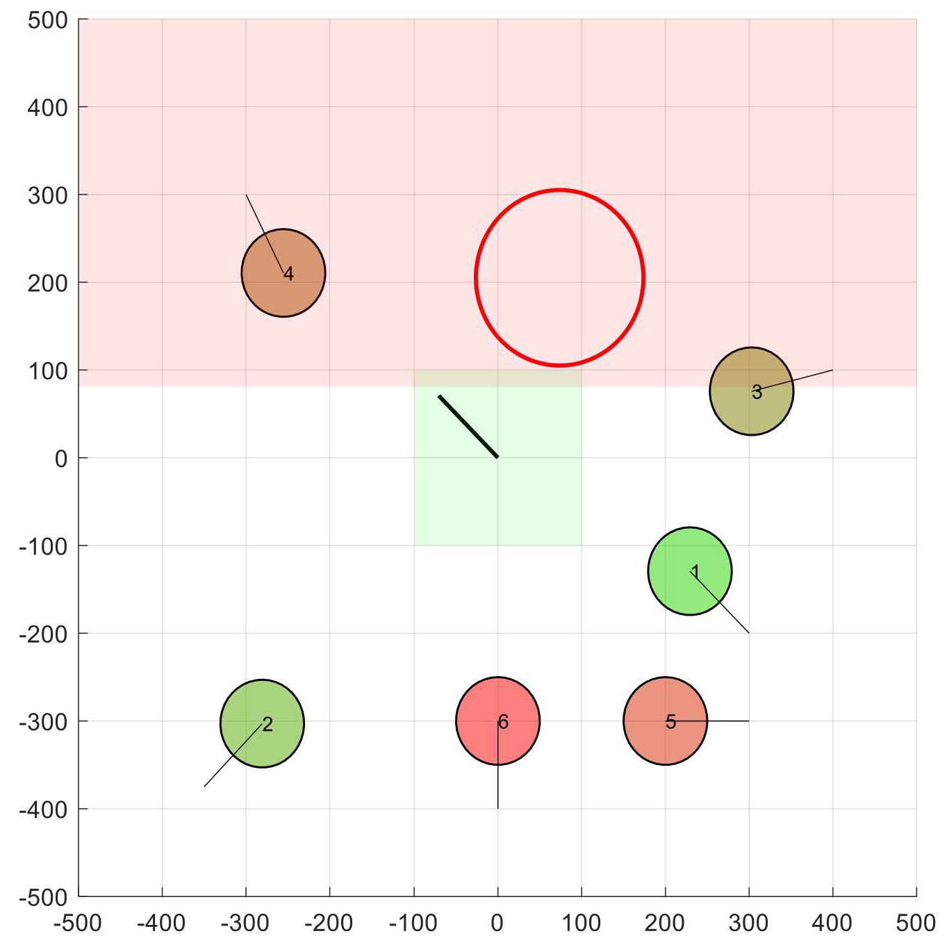
As an illustrative example, Figure 2 shows a scenario with and m. Apart from the 2D location of all nodes (UAVs), the figure shows the velocity space corresponding to node 1. In the origin of coordinates, we can see the initial situation of the green box, assuming m/s.
For each UAV in the neighborhood (line 03 in Table 2), after decomposing it (04), the circular VO that it represents is obtained (05). This VO is then transformed into a quarter-plane (half a half-plane), denoted by a red box (06). Figure 3 shows the circular VO produced by node 3 in node 1, assuming s, and its transformation into a quarter-plane whose north and east ends are located in the infinite. In the figure, the quarter-plane is shown as a red rectangle.
The transformation process applied in (06) is encapsulated in the function detailed in Table 3. This function initially decomposes the circular VO into a position and a radius (14) and obtains the square that inscribes it (15). Then, the vertical and horizontal sides furthest from the center of this square are extended to the infinite (16–25). The function returns the resulting quarter-plane (26).
Once the quarter-plane has been computed, the red box is translated in function of the current velocity of the neighbor node (line 07 in Table 2). Next, the BBCA algorithm acquires the distance from the velocity vector to the respective quarter-plane sides (08). In this calculation, a negative value would indicate the amount of penetration into it. After that, the quarter-plane is extended to obtain a (vertical or horizontal) half-plane (09).
Figure 4 shows the scenario in Figure 3, except that the nodes have already moved towards their destination (which is indicated by a black trace). In addition, the green box shows the velocity vector used by node 1 in the previous iteration. We can see the extension to a half-plane experienced by the quarter-plane.
Table 4 details the way in which a quarter-plane is transformed into a half-plane. First, the distances from the current velocity to the respective sides of the quarter-plane are obtained (27). Next, the side whose distance is greater is chosen (28) and the rest of sides are extended to the infinite (29–36).
Once the half-plane has been obtained, the BBCA algorithm extends it up to half the distance that separates it from the current velocity of the UAV that is running the algorithm (line 10 in Table 2). In this way, both nodes will equally share the responsibility of maneuvering to avoid each other. This allows, among other things, two nodes to fly side by side maintaining the minimum safety distance, instead of repelling each other. Figure 5 shows this operation in the half-plane of Figure 4, although for this example the result is practically imperceptible.
The process carried out by the BBCA algorithm on each UAV in the neighborhood concludes by truncating or trimming the green box (representing the valid velocity space) according to the resulting VO (line 11 in Table 2). Figure 6 shows the result after applying this operation in the situation shown in Figure 5.
Table 5 details this operation. Since the half-plane is implemented with a rectangle with three sides at infinity, the process determines the finite side (41) and truncates the opposite side if needed (42–49).
3.3. Selection of the Final Velocity
Once all these tasks have been performed on all the UAVs in the neighborhood, the final green box representing the valid velocity space for the node running the BBCA algorithm is available. The next action to take will be to determine a specific velocity from among the possible ones and apply it during the following time interval (line 13 in Table 2). Table 6 details this procedure.
Before handling the general case, the procedure deals with two particular cases. Firstly, a null final velocity vector is set (51). The first case corresponds to the situation in which the UAV has reached its destination (52), in which case the procedure concludes (53). At this point, a descent and landing maneuver would be initiated independently of the navigation algorithm. Otherwise, the green box (55) is broken down for analysis. The second particular case may occur in very dense traffic situations, where velocity obstacle-based navigation algorithms get a negative valid velocity space (56). This situation could be visually interpreted as if the green box were folded over itself. Then, there is not a velocity vector guaranteeing the absence of conflict. This problem is minimized by selecting a velocity equidistant from the respective edges (57) and the procedure concludes (58). If none of the particular cases described are in place, the general case has been reached. In this case, the procedure obtains the remaining trajectory vector (60) and uses it to determine the optimal direct velocity to the destination (61). If this velocity is valid, it is found inside the green box (62), then it is set as the final velocity (63) and the process concludes (64). Figure 7 shows an example.
If a direct velocity is not permissible, then we need to determine a vector that is. To do this, we analyze 12 points resulting from geometrically comparing the maximum velocity circle (hereinafter referred to as “the circle”) and the green box representing the valid velocity space (hereinafter referred to as “the box”). First, we would determine the cut points between the circle and the box, both vertically (66) and horizontally (67). In each direction it may be that the circle does not intersect the box but the extension of its sides, in which case (68) it is eliminated as a candidate (69). Visually, this fact means that the candidate point is outside the bounds of the box. Table 7 shows the function that performs this check. If, on the other hand, the intersection is real, this can be a single tangential intersection, or unfolded at two intersections (denoted as positive and negative, respectively). Both situations are handled according to the second option, in which both points would match. We also consider the four vertices of the box (71) as candidates if they are inside the circle (72), discarding them otherwise (73). Note that of the 12 points checked, only 4 to 8 will be maintained, as for each accepted vertex two intersections will be discarded. Figure 8 shows two examples with the twelve candidate points.
Starting from the set of candidate points, the procedure selects the most suitable one. For each candidate velocity vector (75), drift is determined from the ideal vector (76) and it is compared to the best option so far. In case of providing a higher net velocity or, at equal velocity, a better direction towards the destination (77), then it will be considered the best option (78 to 79). This criterion allows other UAVs to be surrounded, instead of colliding with them. Figure 9 shows two examples of choosing the best point among the possible ones.
3.4. Robustness and Safety Margins
In the previous sections, it has been assumed that the UAVs will follow (without margin of error) the paths provided by the navigation system. In this section, we analyze the robustness of the algorithm to possible errors due to “external” factors, such as the presence of gusty winds. Other “internal” factors, such as calculation errors (or excessive latencies) in the geolocation process, or even in the path tracking process itself, should be addressed from a different perspective.
The airspace manager is responsible for estimating the magnitude of these external disturbances and adjusting the algorithm parameters to establish a safety margin, which is determined by the expression . The difference between the conflict detection radius and the distance a UAV can travel during an iteration determines the safety margin. In the next iteration, the navigation system will detect the error and will provide an updated trajectory.
Additionally, the BBCA algorithm is a memoryless process. In this way, it does not assume the correct follow-up of the instructions provided in previous iterations. On the contrary, each node recalculates its trajectory from its current location, the destination location, and the location of the neighboring nodes. Consequently, the algorithm is highly robust. If the nodes suffer unexpected translations, BBCA continues navigating towards the destination, without collapsing or trying to recover the lost trajectory.
4. Simulation Results
In this section we analyze the performance of the proposed collision-free navigation algorithm. First, we study the case in which two UAVs would collide with different relative angles. Then, we focus on the behavior of groups of UAVs with different sizes, where each UAV follows a randomly generated path. In all cases, a standardized evaluation will be carried out by comparing the behavior of the proposed algorithm (referred to as “BBCA”) with the optimal straight-line path without collision avoidance (referred to as “direct”) and with a straightforward implementation of a generic Artificial Potential Field algorithm (referred to as “APF”).
4.1. Two-UAV Study
This subsection analyzes the behavior of the BBCA algorithm in a situation , where both UAVs collide depending on the relative angle that their respective trajectories maintain. Figure 10 shows the different scenarios proposed. Given the circumference of a radius of 1 km, a UAV starts from the west () towards the opposite point of the circumference (w). On the other hand, a UAV has 18 different starting points () ranging from 0° to 170° with a 10° interval, associated to the respective target points (). Both nodes start moving simultaneously with a constant velocity of 13.9 m/s (50 km/h), so they will collide at the center of the circumference if the navigation algorithm does not prevent it. A safety radius of 50 m is applied to both nodes, which will cause a pre-crash conflict, at a time that depends on the relative starting angle.
The results obtained for this initial study are shown below. Figure 11 shows on the abscissa axis the scenario number corresponding to the simulation of the two UAVs with the relative paths described above. The ordinate axis represents the number of collisions produced. The series represent the results obtained by the direct and BBCA algorithms, respectively. As expected, the direct algorithm generates conflicts in all paths. On the contrary, the BBCA algorithm manages to avoid them in all the proposed scenarios.
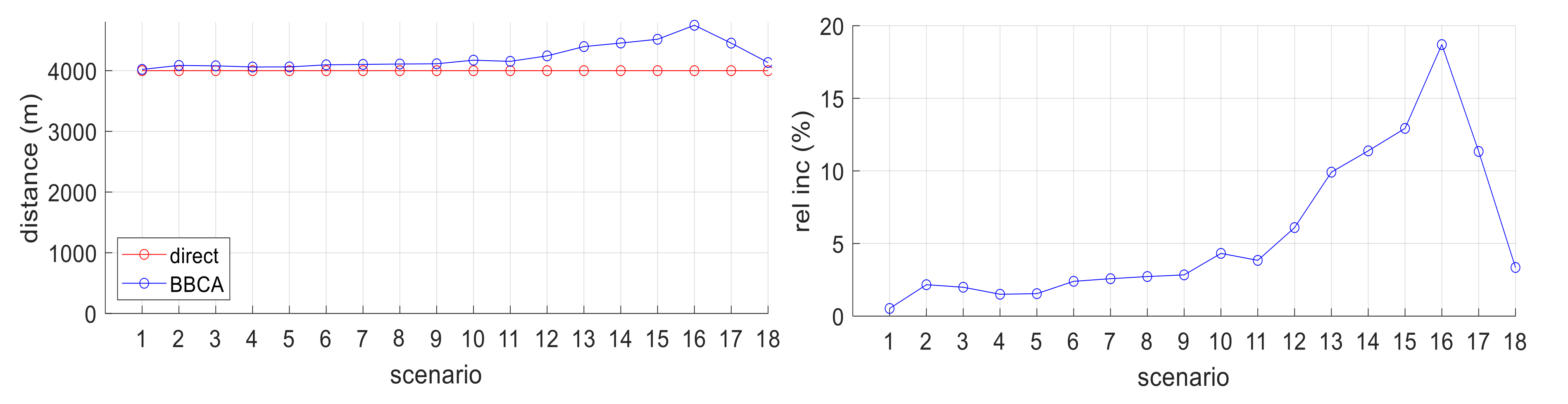
The BBCA algorithm manages to avoid the conflict by making the UAVs deviate from their optimal path, with a consequent increase in the distance travelled and time taken to finally reach their destination. Figure 12 (left) shows on the abscissa axis the scenario number and on the ordinate axis the average distance covered by the UAVs, expressed in meters. The series corresponding to the direct algorithm establishes the minimum route between origin and destination. The BBCA series shows the detour made to avoid the collision, which results in an increase in the distance travelled.
Figure 12 (right) shows the relative results. The abscissa axis represents the scenario number and the ordinate axis shows the relative increase in the distance travelled by the UAVs when the BBCA algorithm is in place (with respect to the direct algorithm). As it can be seen, when the UAVs fly on opposite trajectories, the accumulated deviation by both nodes is around 3%. In the worst case, when the trajectories are almost similar, BBCA causes a detour of no more than 10% (20% accumulated by both nodes) to avoid the conflict. This amount is not exaggerated if we consider that the nodes do not modify their velocity. Given a UAV that stopped in the air, a second UAV located 100 m away that wanted to reach the other end would have to travel 200 m in a straight line (colliding with the first UAV), or 628 m in a curve (in case of going around it).
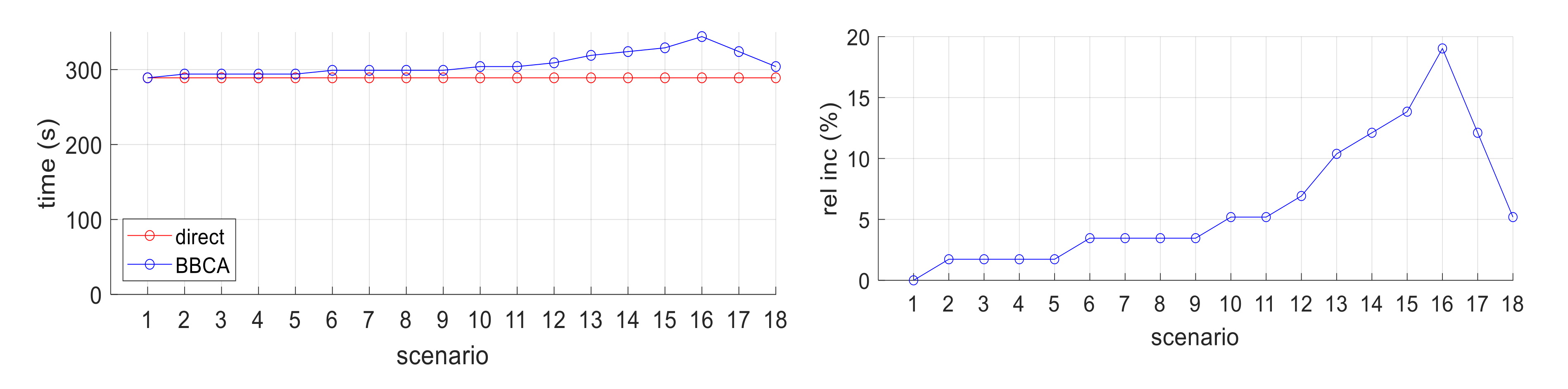
Next, the average time required by the UAVs to perform their maneuvers is analyzed. Figure 13 (left) shows on the abscissa axis the scenario number and on the ordinate axis the average time consumed, expressed in seconds, for each algorithm. The plot on the right relativizes the results obtained by both algorithms. As it can be seen, the time spent is almost proportional to the distance travelled; however, very close values tend to equal each other. This is due to the periodic way in which the navigation mechanism is run. In each cycle, the system provides the highest possible velocity. However, on the last leg, the algorithm reduces the velocity to reach the destination using the full time slot. In the next iteration, the algorithm concludes that it is over the destination, moving them from the navigation phase to the landing phase.
4.2. Multi-UAV Study
In this subsection we analyze the behavior of the BBCA algorithm when it is applied to groups of UAVs of different sizes, flying over an area of km. In particular, . In each case, 24 different configurations have been generated with random start and destination positions uniformly distributed with the following restrictions: (1) UAVs must be more than 100 m from the flying area edge; (2) the length of the route followed by each UAV must be at least 1 km. Each configuration has been tested using the direct, APF, and BBCA algorithms, respectively, requiring a total of 720 simulations. In all cases, a maximum velocity km/h and a safety radius m have been considered. Figure 14 shows two examples.
In Figure 15 (left), the abscissa axis indicates the number of UAVs distributed across the flying area. The ordinate axis shows the average value (and standard deviation) of the collisions produced in the 24 simulated configurations. Without the application of a conflict management mechanism (direct), conflicts increase exponentially with the number of UAVs. A generic APF handles isolated conflicts correctly, but its performance dramatically decreases when they affect to multiple UAVs simultaneously. On the contrary, the use of the BBCA algorithm implies a considerable reduction in conflicts compared to not using it. Figure 15 (right) shows that BBCA obtains a reduction in conflicts of around 90% in the worst case.
Next, we study the penalty in terms of distance travelled and time spent when BBCA is applied, in a similar way to the study carried out for two UAVs. In Figure 16 (left), the abscissa axis indicates the number of UAVs in the flying area and the ordinate axis shows the distance travelled. Each series shows the average and standard deviation of the values obtained in the different configurations. In the absence of conflict management, the expected situation occurs: the average distance travelled by the UAVs remains constant while the deviation decreases as the size of the group of UAVs increases. On the contrary, the detours introduced by APF and BBCA produce an increase with linear behavior in the distance travelled. Figure 16 (right) shows the relative increase in the distance travelled by UAVs. The linearity in the growth of the routes can be clearly seen. Even in extremely dense configurations, where the algorithm avoids 90% of the collisions, it can be said that the penalty of the distance travelled by UAVs is not excessive.
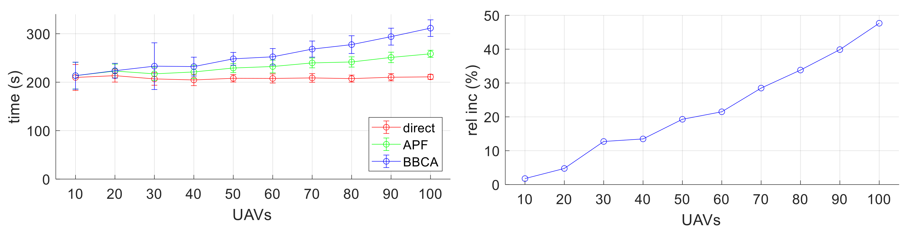
Figure 17 shows the time taken by the UAVs to reach their destination depending on the navigation algorithm used. In both plots, the abscissa axis represents the number of UAVs in the flying area. In the left plot, the ordinate axis represents the time required by the UAVs to reach their destination. Each point corresponds to the average value (and standard deviation) of all the UAVs deployed in a configuration and for the various configurations generated with the same number of UAVs. In the right plot, the ordinate axis represents the relative increase introduced by the BBCA mechanism with respect to the direct one. We can see a behavior of time analogous to the behavior of distance described above.
5. Conclusions and Future Work
In recent years, the use of UAVs in civil applications has grown exponentially in both quantity and versatility. As technical problems are overcome, current aviation legislation is being adapted to allow these uses at a commercial and private level. One of the challenges in this regard is autonomous navigation and, in particular, the real-time management of conflicts (potential collisions) between UAVs.
This paper presents a detailed description and evaluation of an autonomous navigation algorithm with conflict management called BBCA (bounding box collision avoidance). This proposal can be categorized as a simplified version of the popular velocity obstacle method. The simplification consists of limiting the set of generic polygons used to determine the immediate valid region to rectangles in the velocity vector space.
The evaluation results show that, in situations of low traffic density, the mechanism has an excellent performance, correctly managing more than 95% of collisions produced, with an assumable cost, both in distance travelled and in the time required by the UAVs in reaching their destination. By forcing the mechanism into unreal situations of extreme traffic density (in which each UAV is involved in an average of four conflicts along its route), it behaves reasonably well, eliminating 88% of the conflicts generated.
In future work, we plan to incorporate into the BBCA mechanism some control over the velocity vector module of the UAVs (not only over their direction). This would allow them to accelerate, slow down, or even stop in the air (in case of multicopters) if necessary, in order to correctly manage all the conflicts generated, regardless of the air traffic density.
Author Contributions
Conceptualization, R.C. and A.B.; Data curation, P.S.; Formal analysis, R.C.; Funding acquisition, R.C. and A.B.; Investigation, P.S. and A.B.; Methodology, R.C. and A.B.; Project administration, R.C. and A.B.; Resources, A.B.; Software, P.S. and R.C.; Supervision, R.C. and A.B.; Validation, A.B.; Visualization, P.S.; Writing—original draft, P.S., R.C. and A.B.; Writing—review and editing, R.C. and A.B. All authors have read and agreed to the published version of the manuscript.
Funding
This research was funded by the Spanish Ministerio de Ciencia, Innovación y Universidades (MCIU) and European Union (EU) under RTI2018-098156-B-C52 grant, and by the Junta de Comunidades de Castilla-La Mancha (JCCM) and EU through the European Regional Development Fund (ERDF-FEDER) under SBPLY/19/180501/000159 grant.
Conflicts of Interest
The authors declare no conflict of interest. The funders had no role in the design of the study; in the collection, analyses, or interpretation of data; in the writing of the manuscript, or in the decision to publish the results.
References
- Shakeri, R.; Al-Garadi, M.A.; Badawy, A.; Mohamed, A.; Khattab, T.; Al-Ali, A.K.; Harras, K.A.; Guizani, M. Design Challenges of Multi-UAV Systems in Cyber-Physical Applications: A Comprehensive Survey and Future Directions. IEEE Commun. Surv. Tutor. 2019, 21, 3340–3385. [Google Scholar] [CrossRef] [Green Version]
- Foumani, M.; Gunawan, I.; Smith-Miles, K. Resolution of deadlocks in a robotic cell scheduling problem with post-process inspection system: Avoidance and recovery scenarios. In Proceedings of the 2015 IEEE International Conference on Industrial Engineering and Engineering Management (IEEM), Singapore, 6–9 December 2015; pp. 1107–1111. [Google Scholar]
- Foumani, M.; Moeini, A.; Haythorpe, M.; Smith-Miles, K. A cross-entropy method for optimising robotic automated storage and retrieval systems. Int. J. Prod. Res. 2018, 56, 6450–6472. [Google Scholar] [CrossRef]
- Haddadin, S.; De Luca, A.; Albu-Schaffer, A. Robot Collisions: A Survey on Detection, Isolation, and Identification. IEEE Trans. Robot. 2017, 33, 1292–1312. [Google Scholar] [CrossRef] [Green Version]
- Almasri, M.M.; Alajlan, A.M.; Elleithy, K.M. Trajectory Planning and Collision Avoidance Algorithm for Mobile Robotics System. IEEE Sens. J. 2016, 16, 5021–5028. [Google Scholar] [CrossRef]
- Hosseinzadeh Yamchi, M.; Mahboobi Esfanjani, R. Formation control of networked mobile robots with guaranteed obstacle and collision avoidance. Robotica 2017, 35, 1365–1377. [Google Scholar] [CrossRef]
- Phan, D.; Yang, J.; Grosu, R.; Smolka, S.A.; Stoller, S.D. Collision avoidance for mobile robots with limited sensing and limited information about moving obstacles. Form. Methods Syst. Des. 2017, 51, 62–86. [Google Scholar] [CrossRef]
- Zhang, H.; Wang, P.; Zhang, Y.; Li, B.; Zhao, Y. A Novel Dynamic Path Re-Planning Algorithm With Heading Constraints for Human Following Robots. IEEE Access 2020, 8, 49329–49337. [Google Scholar] [CrossRef]
- Tang, J. Conflict Detection and Resolution for Civil Aviation: A Literature Survey. IEEE Aerosp. Electron. Syst. Mag. 2019, 34, 20–35. [Google Scholar] [CrossRef]
- Kuchar, J.K.; Yang, L.C. A review of conflict detection and resolution modeling methods. IEEE Trans. Intell. Transp. Syst. 2000, 1, 179–189. [Google Scholar] [CrossRef] [Green Version]
- International Civil Aviation Organization. Procedures for Air Navigation Services—Air Traffic Management—PANS-ATM Doc 4444; International Civil Aviation Organization: Montreal, QC, Canada, 2009. [Google Scholar]
- GUAN, X.; LYU, R.; SHI, H.; CHEN, J. A survey of safety separation management and collision avoidance approaches of civil UAS operating in integration national airspace system. Chin. J. Aeronaut. 2020. [Google Scholar] [CrossRef]
- Jiang, T.; Geller, J.; Ni, D.; Collura, J. Unmanned Aircraft System traffic management: Concept of operation and system architecture. Int. J. Transp. Sci. Technol. 2016, 5, 123–135. [Google Scholar] [CrossRef]
- Fasano, G.; Accado, D.; Moccia, A.; Moroney, D. Sense and avoid for unmanned aircraft systems. IEEE Aerosp. Electron. Syst. Mag. 2016, 31, 82–110. [Google Scholar] [CrossRef]
- Huang, S.; Teo, R.S.H.; Tan, K.K. Collision avoidance of multi unmanned aerial vehicles: A review. Annu. Rev. Control 2019, 48, 147–164. [Google Scholar] [CrossRef]
- Yasin, J.N.; Mohamed, S.A.S.; Haghbayan, M.-H.; Heikkonen, J.; Tenhunen, H.; Plosila, J. Unmanned Aerial Vehicles (UAVs): Collision Avoidance Systems and Approaches. IEEE Access 2020, 8, 105139–105155. [Google Scholar] [CrossRef]
- Jenie, Y.I.; van Kampen, E.-J.; Ellerbroek, J.; Hoekstra, J.M. Taxonomy of Conflict Detection and Resolution Approaches for Unmanned Aerial Vehicle in an Integrated Airspace. IEEE Trans. Intell. Transp. Syst. 2017, 18, 558–567. [Google Scholar] [CrossRef] [Green Version]
- Ho, F.; Geraldes, R.; Goncalves, A.; Cavazza, M.; Prendinger, H. Improved Conflict Detection and Resolution for Service UAVs in Shared Airspace. IEEE Trans. Veh. Technol. 2019, 68, 1231–1242. [Google Scholar] [CrossRef]
- Fiorini, P.; Shiller, Z. Motion planning in dynamic environments using velocity obstacles. Int. J. Rob. Res. 1998, 17, 760–772. [Google Scholar] [CrossRef]
- Chakravarthy, A.; Ghose, D. Obstacle avoidance in a dynamic environment: A collision cone approach. IEEE Trans. Syst. Man, Cybern. Part A Syst. Hum. 1998, 28, 562–574. [Google Scholar] [CrossRef] [Green Version]
- Douthwaite, J.A.; Zhao, S.; Mihaylova, L.S. Velocity Obstacle Approaches for Multi-Agent Collision Avoidance. Unmanned Syst. 2019, 7, 55–64. [Google Scholar] [CrossRef] [Green Version]
- Douthwaite, J.A.; Zhao, S.; Mihaylova, L.S. A Comparative Study of Velocity Obstacle Approaches for Multi-Agent Systems. In Proceedings of the 2018 UKACC 12th International Conference on Control (CONTROL), Sheffield, UK, 5–7 September 2018; pp. 289–294. [Google Scholar]
- Tan, C.Y.; Huang, S.; Tan, K.K.; Teo, R.S.H. Three Dimensional Collision Avoidance for Multi Unmanned Aerial Vehicles Using Velocity Obstacle. J. Intell. Robot. Syst. 2020, 97, 227–248. [Google Scholar] [CrossRef]
- van den Berg, J.; Guy, S.J.; Lin, M.; Manocha, D. Reciprocal n-Body Collision Avoidance. In Springer Tracts in Advanced Robotics; Springer: Berlin/Heidelberg, Germany, 2011; Volume 70, pp. 3–19. ISBN 9783642194566. [Google Scholar]
- Niu, H.; Ma, C.; Han, P.; Lv, J. An Airborne Approach for Conflict Detection and Resolution Applied to Civil Aviation Aircraft based on ORCA. In Proceedings of the 2019 IEEE 8th Joint International Information Technology and Artificial Intelligence Conference (ITAIC), Chongqing, China, 24–26 May 2019; pp. 686–690. [Google Scholar]
- Daniels, Z.A.; Wright, L.A.; Holt, J.M.; Biaz, S. Collision Avoidance of Multiple UAS Using a Collision Cone-Based Cost Function; Computer Science and Software Engineering Department, Auburn University: Auburn, AL, USA, 2007. [Google Scholar]
- Snape, J.; Guy, S.J.; Lin, M.C.; Manocha, D.; Van Den Berg, J. Reciprocal collision avoidance and multi-agent navigation for video games. In Proceedings of the AAAI Workshop—Technical Report, Toronto, ON, Canada, 22 July 2012; pp. 49–52. [Google Scholar]
- Sun, J.; Tang, J.; Lao, S. Collision Avoidance for Cooperative UAVs With Optimized Artificial Potential Field Algorithm. IEEE Access 2017, 5, 18382–18390. [Google Scholar] [CrossRef]
- Khatib, O. The Potential Field Approach and Operational Space Formulation in Robot Control. In Adaptive and Learning Systems; Springer US: Boston, MA, USA, 1986; pp. 367–377. [Google Scholar]
- Alejo, D.; Cobano, J.A.; Heredia, G.; Ollero, A. Particle Swarm Optimization for collision-free 4D trajectory planning in Unmanned Aerial Vehicles. In Proceedings of the 2013 International Conference on Unmanned Aircraft Systems (ICUAS), Atlanta, GA, USA, 28–31 May 2013; pp. 298–307. [Google Scholar]
- Li, B.; Qi, X.; Yu, B.; Liu, L. Trajectory Planning for UAV Based on Improved ACO Algorithm. IEEE Access 2020, 8, 2995–3006. [Google Scholar] [CrossRef]
- Poli, R. Analysis of the Publications on the Applications of Particle Swarm Optimisation. J. Artif. Evol. Appl. 2008, 2008, 1–10. [Google Scholar] [CrossRef]
- Geng, L.; Zhang, Y.F.; Wang, J.J.; Fuh, J.Y.H.; Teo, S.H. Mission planning of autonomous UAVs for urban surveillance with evolutionary algorithms. In Proceedings of the 2013 10th IEEE International Conference on Control and Automation (ICCA), Hangzhou, China, 12–14 June 2013; pp. 828–833. [Google Scholar]
- Pehlivanoglu, Y.V. A new vibrational genetic algorithm enhanced with a Voronoi diagram for path planning of autonomous UAV. Aerosp. Sci. Technol. 2012, 16, 47–55. [Google Scholar] [CrossRef]
- Li, Y.; Du, W.; Yang, P.; Wu, T.; Zhang, J.; Wu, D.; Perc, M. A Satisficing Conflict Resolution Approach for Multiple UAVs. IEEE Internet Things J. 2019, 6, 1866–1878. [Google Scholar] [CrossRef]
- Dubins, L.E. On Curves of Minimal Length with a Constraint on Average Curvature, and with Prescribed Initial and Terminal Positions and Tangents. Am. J. Math. 1957, 79, 497. [Google Scholar] [CrossRef]
- Shanmugavel, M.; Tsourdos, A.; White, B.; Żbikowski, R. Co-operative path planning of multiple UAVs using Dubins paths with clothoid arcs. Control Eng. Pract. 2010, 18, 1084–1092. [Google Scholar] [CrossRef]
Figure 1.
Example of Unmanned Aerial Vehicle (UAV) notation.

Figure 2.
Example scenario. Circles represent the position of 6 UAVs. The green box represents the initial valid velocity space for node 1.
Figure 2.
Example scenario. Circles represent the position of 6 UAVs. The green box represents the initial valid velocity space for node 1.

Figure 3.
Velocity obstacle (VO) produced by node 3 in node 1.

Figure 4.
Half-plane produced by node 3 in node 1.

Figure 5.
Extension of the obstacle produced by node 3 according to the velocity vector of node 1.

Figure 6.
Valid velocity space truncated (node 1 against node 3).

Figure 7.
Direct velocity to the destination. The black radius (southeast bound) corresponds to the current velocity. The blue radius (south bound) is the direct velocity, which in this case becomes final since it is found inside the green box.
Figure 7.
Direct velocity to the destination. The black radius (southeast bound) corresponds to the current velocity. The blue radius (south bound) is the direct velocity, which in this case becomes final since it is found inside the green box.

Figure 8.
Twelve candidate points: eight cutting points (left) and four corner points (right).

Figure 9.
Choosing the best velocity among the candidate points. In both cases, the red circle delimits the maximum velocity; the green box defines the set of valid velocities; the black radius indicates the current velocity; the blue radius indicates the direct velocity to the destination; the green radius indicates the velocity finally selected for the next time slot.

Figure 10.
Two UAV scenarios: relative path angle.

Figure 11.
Two-UAV study: conflicts produced.

Figure 12.
Two-UAV study: distance covered; absolute values (left) and relative increment (right).

Figure 13.
Two-UAV study: flying time; absolute values (left) and relative increment (right).

Figure 14.
Random scenarios with 30 (left) and 50 (right) UAVs applying BBCA. Numbers in the plots represent initial UAV positions; circles represent current UAV positions and the established safety radius; each line represents a UAV trajectory (from the initial to the final position).
Figure 14.
Random scenarios with 30 (left) and 50 (right) UAVs applying BBCA. Numbers in the plots represent initial UAV positions; circles represent current UAV positions and the established safety radius; each line represents a UAV trajectory (from the initial to the final position).

Figure 15.
Multi-UAV study: conflicts produced; average and standard deviation values (left), and relative decrement of BBCA related to “direct” (right).
Figure 15.
Multi-UAV study: conflicts produced; average and standard deviation values (left), and relative decrement of BBCA related to “direct” (right).

Figure 16.
Multi-UAV study: distance covered; average and standard deviation values (left) and relative increment of BBCA related to “direct” (right).
Figure 16.
Multi-UAV study: distance covered; average and standard deviation values (left) and relative increment of BBCA related to “direct” (right).

Figure 17.
Multi-UAV study: flying time; average and standard deviation values (left) and relative increment (right).
Figure 17.
Multi-UAV study: flying time; average and standard deviation values (left) and relative increment (right).


Table 1.
Conflict detection function.
| 01 | |
| 02 | |
| 03 | if then |
| 04 | |
| 05 | else |
| 06 | |
| 07 | end if |
Table 2.
Bounding box collision avoidance (BBCA) algorithm.
| 01 | |
| 02 | |
| 03 | for all do |
| 04 | |
| 05 | |
| 06 | |
| 07 | |
| 08 | |
| 09 | |
| 10 | |
| 11 | |
| 12 | end do |
| 13 |
Table 3.
Quarter-plane VO.
| 14 | |
| 15 | |
| 16 | if then |
| 17 | |
| 18 | else |
| 19 | |
| 20 | end if |
| 21 | if then |
| 22 | |
| 23 | else |
| 24 | |
| 25 | end if |
| 26 |
Table 4.
Half-plane VO.
| 27 | |
| 28 | case of |
| 29 | : |
| 30 | |
| 31 | : |
| 32 | |
| 33 | : |
| 34 | |
| 35 | : |
| 36 | |
| 37 | end case |
Table 5.
Valid velocity space truncation.
| 38 | |
| 39 | |
| 40 | |
| 41 | case of |
| 42 | : |
| 43 | |
| 44 | : |
| 45 | |
| 46 | : |
| 47 | |
| 48 | : |
| 49 | |
| 50 | end case |
Table 6.
Velocity selection.
| 51 | |
| 52 | if then |
| 53 | return |
| 54 | end if |
| 55 | |
| 56 | if or then |
| 57 | |
| 58 | return |
| 59 | end if |
| 60 | |
| 61 | |
| 62 | if then |
| 63 | |
| 64 | return |
| 65 | end if |
| 66 | |
| 67 | |
| 68 | if not then |
| 69 | |
| 70 | end if |
| 71 | |
| 72 | if then |
| 73 | |
| 74 | end if |
| 75 | for all do |
| 76 | |
| 77 | if or ( and ) then |
| 78 | |
| 79 | |
| 80 | end if |
| 81 | end do |
Table 7.
Valid velocity test.
| 82 | |
| 83 | |
| 84 | if and then |
| 85 | |
| 86 | else |
| 87 | |
| 88 | end if |
© 2020 by the authors. Licensee MDPI, Basel, Switzerland. This article is an open access article distributed under the terms and conditions of the Creative Commons Attribution (CC BY) license (http://creativecommons.org/licenses/by/4.0/).
Share and Cite
MDPI and ACS Style
Sánchez, P.; Casado, R.; Bermúdez, A. Real-Time Collision-Free Navigation of Multiple UAVs Based on Bounding Boxes. Electronics 2020, 9, 1632. https://0-doi-org.brum.beds.ac.uk/10.3390/electronics9101632
AMA Style
Sánchez P, Casado R, Bermúdez A. Real-Time Collision-Free Navigation of Multiple UAVs Based on Bounding Boxes. Electronics. 2020; 9(10):1632. https://0-doi-org.brum.beds.ac.uk/10.3390/electronics9101632
Chicago/Turabian StyleSánchez, Paloma, Rafael Casado, and Aurelio Bermúdez. 2020. "Real-Time Collision-Free Navigation of Multiple UAVs Based on Bounding Boxes" Electronics 9, no. 10: 1632. https://0-doi-org.brum.beds.ac.uk/10.3390/electronics9101632
Note that from the first issue of 2016, this journal uses article numbers instead of page numbers. See further details here.