Article

An Efficient Hardware Architecture with Adjustable Precision and Extensible Range to Implement Sigmoid and Tanh Functions

1
School of Electronic Science and Engineering, Nanjing University, Nanjing 210023, China
2
The KTH Royal Institute of Technology, Kista, 16440 Stockholm, Sweden
*
Authors to whom correspondence should be addressed.
Submission received: 28 September 2020 / Revised: 9 October 2020 / Accepted: 15 October 2020 / Published: 21 October 2020
(This article belongs to the Section Artificial Intelligence Circuits and Systems (AICAS))

Abstract

:
The efficient and precise hardware implementations of tanh and sigmoid functions play an important role in various neural network algorithms. Different applications have different requirements for accuracy. However, it is difficult for traditional methods to achieve adjustable precision. Therefore, we propose an efficient-hardware, adjustable-precision and high-speed architecture to implement them for the first time. Firstly, we present two methods to implement sigmoid and tanh functions. One is based on the rotation mode of hyperbolic CORDIC and the vector mode of linear CORDIC (called RHC-VLC), another is based on the carry-save method and the vector mode of linear CORDIC (called CSM-VLC). We validate the two methods by MATLAB and RTL implementations. Synthesized under the TSMC 40 nm CMOS technology, we find that a special case A R V R ( 3 , 0 ) , based on RHC-VLC method, has the area of 4290.98 μ m 2 and the power of 1.69 mW at the frequency of 1.5 GHz. However, under the same frequency, A R V C ( 3 ) (a special case based on CSM-VLC method) costs 3196.36 μ m 2 area and 1.38 mW power. They are both superior to existing methods for implementing such an architecture with adjustable precision.

1. Introduction

Artificial neural networks (ANNs) are widely used in the applications of pattern recognition, image classification, biological systems and so on [1]. In the past, ANNs were generally implemented only in software. But in recent years, with the development of artificial intelligence and integrated circuits, their hardware implementations have become more and more important because of the performance gains compared with software implementations. In ANNs, each layer or component is important, mainly including convolution, pooling, full connection and activation function. The activation functions can introduce nonlinear factors to neurons, so that the ANNs can approximate any nonlinear functions and be applied to nonlinear models. Therefore, an efficient and accurate implementation of non-linear activation functions, such as t a n h and s i g m o i d , is of high interest.
The t a n h and s i g m o i d functions both shape like an “S” curve, where the outputs of t a n h vary between ( 1 , 1 ) and the range of s i g m o i d outputs is ( 0 , 1 ) . Mathematically, their functions are defined below ( S ( x ) s i g m o i d function, T ( x ) t a n h function).
S ( x ) = 1 1 + e x , T ( x ) = e x e x e x + e x .
In fact, the t a n h function can be converted to:
T ( x ) = e x e x + e x e x e x + e x = 1 2 e x e x + e x .
By dividing numerator and denominator by e x , Equation (2) can be rewritten as:
T ( x ) = 1 2 1 + e 2 x = 1 2 S ( 2 x ) .
It follows that they are functionally related, as above, which enables them to be implemented in a unified architecture. From the formulas, we know that the exponential terms are the key factors that generate the nonlinear behavior. Meanwhile, the accuracy and hardware cost of exponential and division operations can influence the performance of whole neural networks [2,3]. Up to now, some methods have been put forward to solve their implementation problems and can be divided into the following types: look-up tables (LUT) or range addressable LUT (RALUT)-based methods [4,5,6,7], piecewise linear (PWL)-based methods [8,9,10,11], piecewise nonlinear (PWNL)-based methods [12,13] and Taylor series (TS)-based methods [14].
The LUT- or RALUT-based methods take the advantage of look-up tables to store large amounts of points or range values, respectively. Take the LUT-based method as an example it approximates t a n h or s i g m o i d functions with a finite number of distributed points. In general, these points are evenly distributed, or not evenly distributed. The number of points is related to the number of bits used in hardware implementation and it determines the maximum error or average error of results. The biggest advantage of this method is the short latency and it usually just needs one clock cycle. However, its biggest disadvantage is that it requires a lot of memory to store the lookup table. The larger the input range of the computation, or the higher the precision of the results, the larger the memory requirements, which is obviously not desirable in hardware implementations.
Similarly, PWL-based methods use some straight lines to simplify the nonlinear curves of the functions, and the accuracy depends on the number of lines. Compared with LUT- or RALUT-based methods, this method does not store massive data and requires less memory. However, the essence of transforming non-linear behavior into linear behavior makes its accuracy not very high. Especially at the inflection point of the function curve, the number of segments needs to be increased to obtain better accuracy. More segmentations means more storage, and more complex judgment logic. On the other hand, its fitting linear segment formula is as follows: y = k 1 + k 2 × x , where one multiplier is used. As we know, the multiplier is complicated in hardware implementation because of the negative effect on circuit throughput and area utilization. In many designs, it is difficult to accelerate the working frequency because of the existence of the multiplier. Therefore, it is preferable to avoid using multipliers.
By contrast, PWNL-based methods use nonlinear approximation in each segment. Similar to the PWL-based method, it is fitted by the following nonlinear formula: y = k 1 + k 2 × x + k 3 × x 2 + + k n × x n 1 , where the nth order needs ( n + 1 ) n / 2 multiplication operations. The main advantage of this method is that it can achieve higher precision than the PWL-based method. However, a lot of multiplications result in a low working frequency for the whole architecture [12].
The TS-based method faces the same challenges as LUT- or RALUT-based methods. Its accuracy can not be very high because it is limited by the chosen range.
Therefore, it is difficult for each of the above methods to achieve all the advantages of computing t a n h and s i g m o i d functions: high hardware efficiency, adjustable precision, extensible input range, and high computation speed. If we use these methods to build such an hardware architecture, they will be very costly. However, when designing a universal reconfigurable accelerator (such as RASP [15]), it usually includes many operators, such as t a n h and s i g m o i d . If the operator has adjustable precision and the above advantages, it will be very useful. Thus, our proposed architectures to implement t a n h and s i g m o i d have important application value. On the whole, we make the following contributions:
  • For the first time, we propose a hardware architecture with adjustable precision and extensible input range to implement t a n h and s i g m o i d functions, which is based on the RHC-VLC method. In addition, we propose another architecture with unlimited input range and adjustable accuracy, which is based on CSM-VLC method.
  • Of the two proposed methods, the accuracy magnitude based on the CSM-VLC method can reach 10 4 best, while the magnitude of the accuracy based on the RHC-VLC method can be much better, such as 10 7 or 10 8 . At the same time, the proposed methods can change the accuracy by adjusting the iterations of CORDIC without changing the current computing architecture. The lower the accuracy requirement, the lower the overall latency. Other methods of adjusting the precision require architectural changes, which are extremely unfriendly in hardware implementation.
  • In hardware implementation, the RHC-VLC-based method only requires shift-and-add (or subtract) operations. Another method based on CSM-VLC requires a constant multiplier, we also optimize it to achieve shorter delay and smaller area. Compared with other existing methods to implement a hardware architecture with adjustable precision, our hardware implementation is more efficient. The proposed architecture has dual computing capabilities ( t a n h and s i g m o i d ), which can be determined by the input selection bit.
  • Under TSMC 40 nm CMOS technology, the hardware architecture based on our proposed methods can work at 1.5 GHz frequency or even higher. Except for the high frequency, our methods are also compatible with other advantages: efficient hardware, adjustable precision, and extensible input range. With the same adjustable range of precision, our architecture has lower area and power consumption compared with other methods.
The rest of this paper is organized as follows. Section 2 details the first proposed architecture based on the RHC-VLC method to implement t a n h or s i g m o i d functions. Section 3 presents another proposed architecture based on the CSM-VLC method. Section 4 shows the general hardware implementation and a specific case of these two methods. Then, we make a comparison with other methods. Finally, Section 5 draws the conclusions.

2. Proposed Architecture Based on RHC-VLC Method

To solve the problem of not being able to build a hardware architecture that has all of the above four advantages, we propose two solutions: The RHC-VLC-based method and CSM-VLC-based method. In this section, we first detail the architecture based on the RHC-VLC-method, including basic theory, method process, software simulation and algorithm construction. Another architecture based on the CSM-VLC method will be presented in the next section.

2.1. Overview of RHC and VLC

Before introducing the first method, we need to review what RHC and VLC are. Only based on this theory can we build an architecture with adjustable precision and extensible input range to compute s i g m o i d and t a n h functions.
In 1959, Volder invented CORDIC to evaluate trigonometric functions, multiplication and division [16]. Later, Walter extended its computation capacities to compute exponentials, logarithms and square roots [17]. In this paper, only VLC and RHC are adopted, so we omit the introduction to other types of CORDIC. Their iterative formulas can be found in [18].
R H C : x k + 1 = x k + ζ · ( 2 k y k ) , y k + 1 = y k + ζ · ( 2 k x k ) , z k + 1 = z k ζ · t a n h 1 ( 2 k ) ,
where ζ = s i g n ( z k ) , k 1 and k are integers. Especially, when the iteration number k = 4 , 13 , 40 , , n , one more iteration of RHC should be required. Otherwise, RHC cannot converge.
V L C : x k + 1 = x k , y k + 1 = y k η · ( 2 k x k ) , z k + 1 = z k + η · 2 k ,
where η = s i g n ( y k ) , k 0 and k is an integer.
After a few iterations, RHC and VLC will converge to some common functions, which are shown in Table 1.
Γ is computed by k = 1 n ( 1 2 2 k ) and called the scale-factor, where the terms ( k = 4 , 13 , 40 , ) should be multiplied again. When the iteration number of RHC is determined, Γ will be a constant value, so we do not need to compute it in actual applications.
From Table 1, we know that RHC has the ability of calculating hyperbolic sine ( s i n h ) and hyperbolic cosine ( c o s h ) if we initialize the inputs as x 0 = 1 / Γ and y 0 = 0 , VLC can implement the division operation if z 0 is initialized to be 0. They all lay the foundation to compute the s i g m o i d and t a n h  functions.

2.2. The RHC-VLC-Based Method

This method of computing S ( x ) contains two steps. The first step deals with the exponential operation of e x , which can be implemented by RHC. Because
c o s h ( x ) + s i n h ( x ) = e x ,
we can initialize the inputs of RHC as follows:
x 0 = 1 / Γ , y 0 = 0 , z 0 = x .
Then, we can get the result of e x through x n plus y n .
The second step handles the division operation, which can be calculated by VLC. To this end, the inputs of VLC are initialized to
x 0 = 1 + e x , y 0 = 1 , z 0 = 0 ,
so the output z n will converge to 1 1 + e x and it is exactly the result of S ( x ) . From the relationship in Equation (1), we can design the architecture shown in Figure 1 to calculate S ( x ) or T ( x ) . “t” represents the functionality to be implemented by the current architecture, t = 0 means computing S ( x ) , and  t = 1 stands for computing T ( x ) .
Since the convergence range of RCH or VLC is limited, we should analyze the range of the input variable x of computing S ( x ) and T ( x ) (called S & T ). As can be intuitively seen from Figure 1, the convergence range of RHC is affected by VLC and the range of input x is determined by RHC.
As for the standard CORDIC, the convergence range of RHC is | z 0 | 1.1182 , and that of VLC is y 0 x 0 1 [19]. Because the output of T ( x ) varies between [−1, 1] and the S ( x ) output varies between [0, 1], their ranges happen to be suitable for VLC, and we do not need to expand the converge range of VLC. Then, we analyze the range of the variable x when we use RHC to compute e x or e 2 x . x belongs to [−1.1182, 1.1182] for computing S ( x ) and x only belongs to [−0.5591, 0.5591] for computing T ( x ) , which are both very limited and not suitable for practical applications.
Therefore, we should expand the range of input variables z 0 of RHC. Hu [19] shows that, if we extend the iteration index set from k = 0 , 1 , , n to k = m , m + 1 , , 0 , , n , the convergence range of RHC will be expanded. However, the iterative formulas will be changed when k 0 , where the terms containing 2 k need to be replaced by 1 2 2 k + 1 . That is
x k + 1 = x k + s i g n ( z k ) ( 1 2 2 k + 1 y k ) , y k + 1 = y k + s i g n ( z k ) ( 1 2 2 k + 1 x k ) , z k + 1 = z k s i g n ( z k ) t a n h 1 ( 1 2 2 k + 1 ) ,
The convergence range of the expanded RHC depends on the maximum sum of rotation angles, which is defined as
θ m a x ( m , n ) = k = m 0 t a n h 1 ( 1 2 2 k + 1 ) + k = 1 n t a n h 1 ( 2 k ) ,
where the terms of iterative number k = 4 , 13 , 40 , should be accumulated twice.
Ulterior to this, the convergence range of RHC will be updated to z 0 θ m a x ( m , n ) , and we can enlarge or reduce the range through changing the value of m. For example, n is assumed to be 15, then we can change the value of m to get different convergence ranges of RHC, including the corresponding input ranges for T ( x ) and S ( x ) , as shown in Table 2.
In consideration of the iterations of the expanded RHC are related to two parameters (let them be m and n, m 0 , n 1 ) and the iterations of VLC are relevant to one parameter (let it be p, p 1 ), we can denote the architecture of computing S & T as A r V L C R H C ( m , n , p ) .

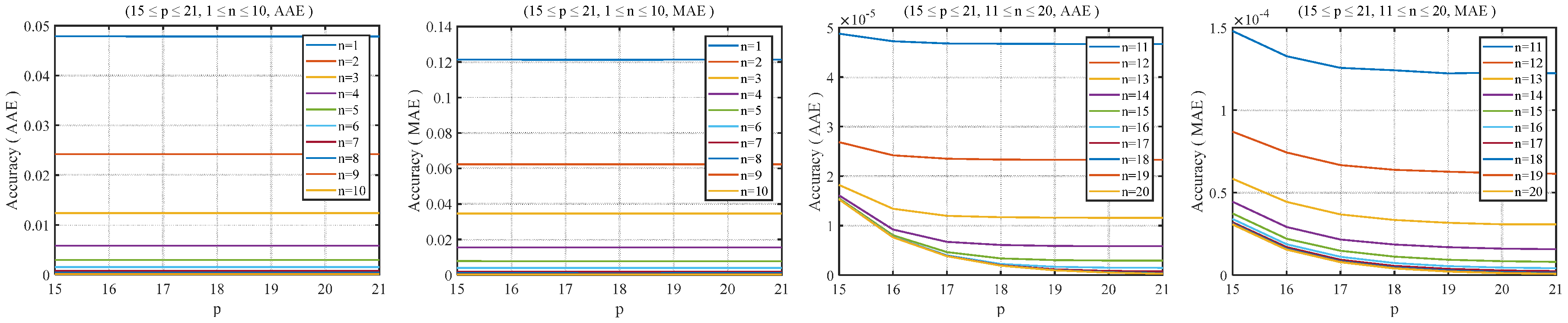
2.3. Software Test for the RHC-VLC-Based Method

Before we go further and design an architecture with adjustable precision, it is necessary to conduct a software simulation for validating and exploring the accuracy of computing S & T . First, we input different data x to verify the correctness of S & T . Then, we explore the accuracy distribution of computing S & T through changing the iterations of VLC and RHC.
In order to evaluate the accuracy of the proposed architecture, we characterize it with maximum absolute error ( M A E ) and average absolute error ( A A E ) and they are defined as:
M A E = m a x ( | V o r i V p r o | i ) , A A E = Σ ( | V o r i V p r o | i ) N U M ,
where 1 i N U M , V o r i stands for the value of original functions, V p r o represents the value of proposed architecture, and N U M means the total test points.
Since the accuracy of RHC and VLC is closely related to the number of iterations, we can first explore the distribution of the respective accuracy of RHC and VLC. All cases set N U M to be 100,000 and the input x is generated by a random number. (Figure 2 and Figure 3 both use logarithmic ordinates.)
The first case: We set the number of iterations (n) of RHC to range from 1 to 20 and the input range is [−1.118, 1.118]. Since all iteration numbers are positive, each iteration of RHC will adopt the iterative formulas, described by Equation (4). As can be seen from Figure 2, when n is greater than 10, the order of magnitude of A A E changes from −4 to −7. The magnitude of M A E varies from −4 to −6 when n is greater than 11. The more times of positive iterations, the higher the accuracy.
The second case: We set the number of negative iterations (m) of RHC to vary from 0 to 4 and the input range is [−2.028, 2.028]. The maximum positive iteration number (n) ranges from 1 to 20. The terms with positive iteration numbers still adopt the iterative formulas, shown as Equation (4), but those with negative iterations will use Equation (9). From Figure 3, we can see that the negative iterations basically do not affect the accuracy of RHC and the order of magnitude of A A E or M A E is the same as Figure 2.
The third case: In order to evaluate the computational accuracy of VLC, we set the number of iterations (p) to scale from 1 to 20 and the input range is [1, 100]. The iterative formulas used in the simulation are shown in Equation (5). The following conclusions can be drawn from Figure 2: The larger the p value, the higher the calculation accuracy of VLC. When p 9 , the order of magnitude of A A E is smaller than −4. However, when M A E reaches the same magnitude, p must be greater than 10.
Next, based on the accuracy of the above two computation modules—RHC and VLC—we use the control variable method to explore the precision distribution of computing S & T . All cases set N U M to be 100,000 and the input x is generated by random number. From Figure 3, we know that the parameter m of RHC has little effect on the accuracy, so we set it to 0 first. In this case, the accuracy of computing S & T is only affected by the iterations n and p. In order to obtain n and p, corresponding to different magnitudes of M A E and A A E , we divide the discussion into three cases. (Input range x: S ( x ) [ 2 , 2 ] and T ( x ) [ 1 , 1 ] .)
Case 1: m = 0 , 1 n 20 , 1 p 7 . The simulation result is shown in Figure 4 and Figure 5. They tell us that, for the same iterations (n and p), the accuracy of t a n h is slightly lower than that of s i g m o i d . Then, when 3 p 7 and 1 n 10 , the accuracy is improved with the increase in p. Finally, if p is small and n is large, the precision stays pretty much the same.
Case 2: m = 0 , 1 n 20 , 8 p 14 . The simulation result is shown in Figure 6 and Figure 7. Similar to Case 1, when 8 p 14 , no matter how n varies in 1 n 10 , the accuracy remains basically the same. However, when n is increased in the range of 11 n 20 , the accuracy is greatly improved. On the whole, the precision under the condition of Case 2 is better than that of Case 1.
Case 3: m = 0 , 1 n 20 , 15 p 21 . The simulation result is shown in Figure 8 and Figure 9. Except for some features common to Case 1 and Case 2, the overall accuracy of Case 3 is higher than that of Case 1 and Case 2 (n in the same range). As p increases, even if n is small or large, the accuracy remains basically the same. As n and p both increase gradually, the precision tends to be of the same magnitude.
From the above experimental results, it can be seen that the computation accuracy of S & T is strongly associated with the combination of RHC and VLC iterations. As long as the iterations of RHC and VLC are determined, the output precision of these two activation functions will be determined accordingly. In this way, the architecture based on the RHC-VLC method is not only with adjustable precision, but is also easy to implement and extend in hardware.

2.4. Proposed Algorithm with Adjustable Precision

Through the simulation verification in the previous subsection, we know the relationship between the computation precision of S & T and the iterations of RHC and VLC. Since different precision magnitudes correspond to multiple combinations of RHC and VLC iterations, we further classify and screen them according to a principle of fewer total iterations (Principle: A A E and M A E are expressed as “ K × 10 E ”, K ϵ ( 1 , 5 ] and E is a negative integer), as shown in Table 3 and Table 4. Here, only partial results corresponding to the order of magnitude of precision are shown. If the magnitude is less than −6, it can be obtained according to the above method, which will not be detailed in this paper.
Next, according to the Section 2.2 and Section 2.3, we propose an algorithm (Algorithm 1) to compute S & T with adjustable precision, which is called the R V S T algorithm in this paper. It can be seen from Table 3 and Table 4, that the accuracy of the same magnitude may correspond to multiple iterative combinations, and it is better to take n smaller and p larger than the criterion. The reason is that according to Equations (4) and (5), the hardware implementation of V L C is less complex than that of R H C . Therefore, the combinations of m, n and p in the R V S T algorithm are determined and they are also the best combinations. The input range is shown in Table 2 and it varies with the value of m. However, the value of m has little effect on the accuracy. In the R V S T algorithm, M A E is used as the accuracy standard. Besides, A A E can also be adopted.
Algorithm 1 R V S T algorithm.
Input: The parameter x that needs to be calculated; the calculated type t ( t = 0 S ( x ) and t = 1 T ( x ) ); the required order of magnitude ( r m ) of M A E (all are positive numbers, for example, 2 actually represents “ 2 ”); m i determines the input range of x
Output: Final result F R
 1:
ift = 0 then
 2:
 if    r m = 2   m = m i , n = 3 , p = 6
 3:
 else if  r m = 3   m = m i , n = 8 , p = 8
 4:
 else if  r m = 4   m = m i , n = 10 , p = 12
 5:
 else if  r m = 5   m = m i , n = 14 , p = 15
 6:
 else        m = 0 , n = 0 , p = 0
 7:
 Return F R = S ( x , m , n , p )
 8:
else
 9:
 if    r m = 2   m = m i , n = 4 , p = 7
  10:
 else if  r m = 3   m = m i , n = 8 , p = 10
  11:
 else if  r m = 4   m = m i , n = 11 , p = 13
  12:
 else if  r m = 5   m = m i , n = 15 , p = 16
  13:
 else        m = 0 , n = 0 , p = 0
  14:
 Return F R = T ( x , m , n , p )
  15:
end if
As can be seen from Algorithm 1, in addition to the conditional statements, there are two functions: S ( ) and T ( ) (more on that below). In general, the algorithm is clear and simple in hardware implementation.
Further, we introduce the algorithm of function S ( ) . The principle of the algorithm is based on Figure 1 and it is termed as S algorithm. It should be noted that the values of 1 / Γ in Figure 1 are different under different iterations of RHC, as shown in Table 5. Another thing to note is that when RHC contains non-positive indexed iterations, the new scale-factor Γ should be redefined as
k = m 0 ( 1 ( 1 2 2 k + 1 ) 2 ) · k = 1 n ( 1 2 2 k )
Similarly, we can derive the algorithm for the function T ( ) from Figure 1, which is called T algorithm. In the hardware implementation, multiplying by 2 is equivalent to moving one bit to the left. For RHC and VLC, only shift-add (or subtract) operations are required. Therefore, Algorithms 1–3, there is no complicated hardware logic, which ensures the efficiency of the whole architecture. Specific hardware implementation of the proposed architecture is detailed in Section 4.
Algorithm 2S algorithm.
Input: The parameter x that needs to be calculated; m, n, and p correspond to the iterations of RHC
and VLC, respectively
Output: S ( ) result S R
 1:
R y 0 = 0
 2:
R z 0 = x
 3:
if     r m = 2  R x 0 = 0.55028235384
 4:
else if   r m = 3  R x 0 = 0.54885034814
 5:
else if   r m = 4  R x 0 = 0.54884903958
 6:
else if   r m = 5  R x 0 = 0.54884895268
 7:
else          R x 0 = 0
 8:
( R x n , R y n , R z n ) = R H C ( R x 0 , R y 0 , R z 0 , m , n )
 9:
V x 0 = R x n + R y n + 1 , V y 0 = 1 , V z 0 = 0
  10:
( V x p , V y p , V z p ) = V L C ( V x 0 , V y 0 , V z 0 , p )
  11:
Return S R = V z p
Algorithm 3T algorithm.
Input: They are the same as S algorithm
Output: T ( ) result T R
 1:
R y 0 = 0
 2:
R z 0 = x · 2
 3:
if      r m = 2  R x 0 = 0.54920653198
 4:
else if    r m = 3  R x 0 = 0.54885034814
 5:
else if    r m = 4  R x 0 = 0.54884897415
 6:
else if    r m = 5  R x 0 = 0.54884895243
 7:
else         R x 0 = 0
 8:
( R x n , R y n , R z n ) = R H C ( R x 0 , R y 0 , R z 0 , m , n )
 9:
V x 0 = R x n + R y n + 1 , V y 0 = 1 , V z 0 = 0
  10:
( V x p , V y p , V z p ) = V L C ( V x 0 , V y 0 , V z 0 , p )
  11:
Return T R = ( 1 V z p ) · 2

3. Proposed Architecture Based on CSM-VLC Method

In this section, we introduce another method based on the CSM (carry-save method) and VLC. The difference between this method and the RHC-VLC-based method is that the latter uses RHC to compute the exponential directly, whereas here the exponential is calculated based on the CSM. Therefore, we focus on how to calculate e x and e 2 x in the following.

3.1. Compute E X and E 2 X

Generally speaking, the expansion of exponential functions in accordance with Taylor’s formula requires a large number of multiplication operations, while the hardware implementation of multiplication not only consumes a lot of logical resources, but it also leads to a long data path delay. In addition, the input range of the exponential functions should not be large, otherwise the data bit width is too large or the precision is not guaranteed in the hardware implementation. Therefore, in order to overcome the above disadvantages, we design a special hardware architecture for e x and e 2 x in t a n h and s i g m o i d functions. First, by means of the mathematical formula transformation, we convert e x and e 2 x into:
e x = 2 ( x ) · l o g 2 e = 2 r 1 , e 2 x = 2 ( 2 x ) · l o g 2 e = 2 r 2 .
When we get the values of r 1 and r 2 , then we can easily separate their integer and decimal parts, assuming: r 1 = I 1 + D 1 , r 2 = I 2 + D 2 , where
I 1 = f l o o r ( ( x ) · l o g 2 e ) , I 2 = f l o o r ( ( 2 x ) · l o g 2 e ) ,
and
D 1 = ( x ) · l o g 2 e f l o o r ( ( x ) · l o g 2 e ) , D 2 = ( 2 x ) · l o g 2 e f l o o r ( ( 2 x ) · l o g 2 e ) ,
f l o o r ( x ) is a function that returns the greatest integer less than or equal to x, which is usually denoted as “ f l o o r ( x ) = [ x ] ”—for example, f l o o r ( 1.2 ) = 2 and f l o o r ( 1.2 ) = 1 . Further, we can simplify Equation (13) as follows:
e x = 2 I 1 + D 1 = 2 I 1 · 2 D 1 = 2 D 1 < < I 1 , f o r I 1 > 0 , 2 D 1 > > ( I 1 ) , f o r I 1 0 , e 2 x = 2 I 2 + D 2 = 2 I 2 · 2 D 2 = 2 D 2 < < I 2 , f o r I 2 > 0 , 2 D 2 > > ( I 2 ) , f o r I 2 0 ,
< < X ” means to move X bit to the left and “ > > Y ” means to move Y bit to the right.
Therefore, two natural exponential functions are transformed into a same exponential function with base 2, and the computation range is changed from “ ( , + ) ” to “[0,1)”, which just needs an extra shift operation. For “ 2 D 1 or 2 D 2 , D 1 , D 2 ϵ [ 0 , 1 ) ”, we can easily implement them according to the required precision by taking advantage of the LUT-based or PWL-based methods.
After introducing the above transformation process, we can obtain the hardware architecture shown in Figure 10, which contains a constant multiplier, an exponential calculator (EC) and a shift unit (SU).
As we mentioned earlier, a multiplier not only consumes a lot of resources in hardware implementation, but also causes long data path delay. So we introduce a method of optimizing the constant multiplier used in this paper, which can greatly reduce its hardware complexity and its critical path. The optimization method includes algorithmic level and architectural level.
First, we talk about the optimization at the algorithmic level. We know that ( x ) · l o g 2 e and ( 2 x ) · l o g 2 e can be written as
( x ) · l o g 2 e = x · l o g 2 1 e , ( 2 x ) · l o g 2 e = x · l o g 2 e 2 ,
where l o g 2 1 e is approximately equal to 1.442695040888963 and l o g 2 e 2 approximates to 2.885390081777927 . We can further get
x · ( 1.442695040888963 ) = x · ( 2 + 0.557304959111037 ) = 2 x + 0.557304959111037 x , x · ( 2.885390081777927 ) = x · ( 2 + 0.885390081777927 ) = 2 x + 0.885390081777927 x .
Then, we introduce the optimization at the architectural level. In binary terms, we know that 0.557304959111037 is approximately ( 0.1000111 ) 2 (= 0.5546875 ) and 0.885390081777927 is approximately ( 0.1110001 ) 2 (= 0.8828125 ). If we design a constant multiplier in the normal way, there will be four shifts and three additions. However, we can simplify it to three shifts or two shifts, one addition and one subtraction, which is called the “3-1-1” or the “2-1-1” method in this paper. The implementation process of this method is as follows.
The above two binary numbers can be further rewritten as:
( 0.1000111 ) 2 = ( 0.1000000 ) 2 + ( 0.0001000 ) 2 ( 0.0000001 ) 2 , ( 0.1110001 ) 2 = ( 1.0000000 ) 2 + ( 0.0000001 ) 2 ( 0.0010000 ) 2 .
In this case, that is
x 1 · ( 0.1000111 ) 2 = x 1 > > 1 + x 1 > > 4 x 1 > > 7 , x 2 · ( 0.1110001 ) 2 = x 2 + x 2 > > 7 x 2 > > 3 .
The top one is “3-1-1”, and the bottom one is “2-1-1” in Equation (20). In general, “one plus and one minus” can be converted to “three plus”; that is, subtracting a number is equal to adding its two’s complement. Then, we turn Equation (20) into:
x 1 · ( 0.1000111 ) 2 = x 1 > > 1 + x 1 > > 4 + ( x 1 > > 7 ) + 1 , x 2 · ( 0.1110001 ) 2 = x 2 + x 2 > > 7 + ( x 2 > > 3 ) + 1 .
Supposing that x 1 and x 2 are all M bits, if we use a traditional method to compute the above formula, 3 M full adders (FAs) are needed and the critical path time is 3 M τ ( τ is the operation time of a full adder). However, we use a method called CSM to reduce both the number of FAs (from 3 M to 2 M ) and the critical path time (from 3 M τ to ( M + 1 ) τ ). Of course, a reduction in the number of FAs means that the area and power consumption of the whole architecture will be also reduced. In fact, we can also consider using the carry select adders [20,21,22] to implement Equation (21), but for the sake of balancing area and speed, we do not adopt it in this paper.
Let the equations for “ x 1 · ( 0.1000111 ) 2 ” and “ x 2 · ( 0.1110001 ) 2 ” look like “ I 1 + I 2 + I 3 + 1 ” and let their results be expressed in terms of “R”, the optimized architecture for computing 0.5546875 x 1 or 0.8828125 x 2 , as is shown in Figure 11.

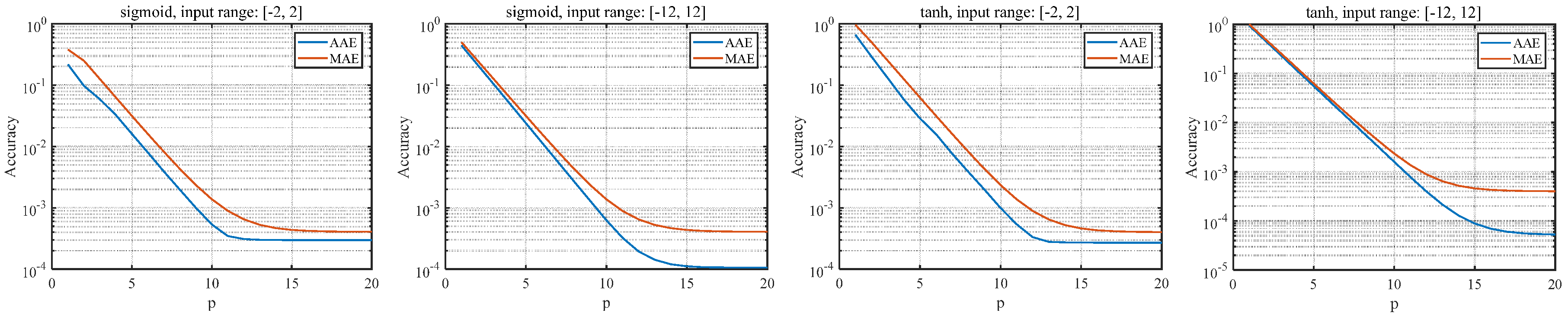
3.2. Software Test for the CSM-VLC-Based Method

Now, we use the accuracy criteria ( A A E and M A E ) to evaluate the precision of this method. Compared with the method based on RHC-VLC, the CSM-VLC-based method has a wider input range. Although there is no scope limitation in nature, we still set two limited test input ranges: [ 2 , 2 ] and [ 12 , 12 ].
Since the iterations (p) of VLC can be set flexibly, the precision of division operation will also change accordingly. Therefore, we set the parameter p from 1 to 20 to explore the accuracy of computing S & T with the CSM-VLC-based method. The final simulation results can be obtained through MATLAB, as shown in Figure 12. (It uses logarithmic ordinate.)
From Figure 12, we can draw the following conclusions: (1) with the increase in p, the accuracy of computing S & T with this method becomes higher; (2) the greater the p value, the more the accuracy tends to remain unchanged; (3) the larger the input range and the larger the p value, the higher the accuracy; (4) compared with the method based on RHC-VLC, the overall computation accuracy of this method is not dominant; (5) the input range of this method is essentially unlimited, but the RHC-VLC-based method needs to adjust the iterations of RHC to expand the input range, so the architecture based on CSM-VLC is superior in this respect.

3.3. Proposed Algorithm with Adjustable Precision

Through the previous simulation verification, we obtain the relationship between the computation accuracy of S & T and the iterations of VLC. Since different precision magnitudes correspond to different iterations of VLC, we first classify and screen them according to a principle of fewer iterations. (Principle: A A E and M A E are expressed as “ K × 10 E ”, K ϵ ( 1 , 5 ] and E is a negative integer), as shown in Table 6. From Figure 12, we know that even if the p value becomes larger, it is difficult to improve the accuracy by another magnitude. Therefore, only M I V corresponding to three kinds of accuracy magnitude are shown in the Table 6, which also lays the foundation for another proposed algorithm based on CSM-VLC with adjustable precision.
According to the final optimization of e x and e 2 x and Table 6, we can obtain another new algorithm (based on CSM-VLC) to compute S & T , which is called the C V S T algorithm (Algorithm 4) in this paper. The specific implementation of V L C ( ) in this algorithm refers to the previous algorithm. In the C V S T algorithm, we use M A E as the accuracy standard and of course, we can also adopt A A E .
Algorithm 4 C V S T algorithm.
Input: They are the same as R V S T algorithm
Output: Final result F R
 1:
ift = 0 then
 2:
V = 2 x + 0.5546875 x
 3:
 if     r m = 2    p = 5
 4:
 else if   r m = 3    p = 8
 5:
 else if   r m = 4    p = 14
 6:
 else          p = 0
 7:
else
 8:
V = 2 x + 0.8828125 x
 9:
 if     r m = 2    p = 6
  10:
 else if   r m = 3    p = 9
  11:
 else if   r m = 4    p = 15
  12:
 else          p = 0
  13:
end if
  14:
I n t = f l o o r ( V )
  15:
F r a = V f l o o r ( V )
  16:
V x 0 = 2 I n t · 2 F r a , V y 0 = 1 , V z 0 = 0
  17:
( V x n , V y n , V z n ) = V L C ( V x 0 , V y 0 , V z 0 , p )
  18:
ift = 0 then
  19:
 Return F R = V z n
  20:
else
  21:
 Return F R = 1 V z n · 2
  22:
end if

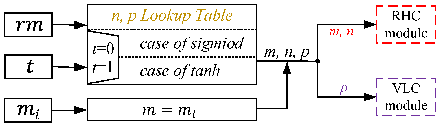
4. Hardware Implementation

After proposing two algorithms with adjustable accuracy to calculate S & T functions, and learning their advantages and disadvantages through software simulation, we further compare their pros and cons through specific hardware implementations, including the comparison with other methods.
For the convenience of expression, we denote the hardware architecture of R V S T algorithm as A R V R ( r m , m i ) . Similarly, the C V S T algorithm in hardware implementation is named A R V C ( r m ) . Here, r m refers to the magnitudes of M A E and m i determines the range of input x.

4.1. General Architecture Based on RHC-VLC Method

According to the R V S T algorithm, we can design two structures: one is a non-pipelined structure, which can save a lot of hardware area. The other is a pipelined structure, which can obtain high throughput. In this paper, all hardware designs adopt the pipelined structure.
The general architecture A R V R ( r m , m i ) is shown in Figure 13, which mainly includes PS (precision selector) module, RHC module, VLC module and Adder. When the inputs ( x , t , r m , m i ) are valid, the sign bit of x will flip if t = 0 , otherwise, x will be shifted left for one bit as with the initial input z 0 of the RHC module. The PS module selects the corresponding iterations ( m , n , p ) according to the values of r m , m i and t, then it transmits them to the RHC module and the VLC module, respectively. After a fixed number of iterations, the output of RHC module is valid, x n and y n of RHC will be added up by adder and used as the initial input x 0 of the VLC module. Similarly, when the output of the VLC module is valid, if t = 1 , z p will convert its sign bit and then be shifted one bit to the left, the result is added up by 1 as the final result of T ( x ) . However, if t = 0 , z p will be directly the final result of S ( x ) .
Next, we detail the architecture of each module, namely the PS module, RHC module and VLC module. First, we introduce the PS module, as shown in Figure 14. Since m i determines the input range of x, which is independent of the current function to be calculated and does not affect the calculation accuracy, it is directly equal to m. The values of r m and t determine the different combinations of n and p. m and n are transmitted to the RHC module and p to the VLC module. See Table 3 and Table 4 for “ c a s e o f s i g m o i d ” and “ c a s e o f t a n h ”.
Figure 15 shows that the inputs and outputs of each iteration of VLC are cascaded back and forth. The kth stage includes the shift operations, which needs to shift x k by k bits to the right. The constants contained in the look-up table are calculated by 2 k . In the same way, Figure 16 describes a pipelined architecture of RHC module. Unlike the VLC module, there are two kinds of architecture in the RHC module. One is the RHC of positive iterative number (called P-RHC), another is that of the non-positive iterative number (called NP-RHC). For the P-RHC, the kth stage needs to shift x k and y k by k bits to the right and the constants in Lookup Table 2 are computed by t a n h 1 ( 2 k ) . However, the kth stage of NP-RHC should shift x k and y k by 2 1 k bits to the right and the elements in Lookup Table 3 are calculated by t a n h 1 ( 1 2 2 k + 1 ) . There are seven cases of the initial value x 0 , the specific constant values are shown in Table 5 and stored in Lookup Table 1.

4.2. General Architecture Based on CSM-VLC Method

Different from A R V R ( r m , m i ) , the input m i is no longer needed in A R V C ( r m ) . In the PS module, there can be no case of r m 5 because the upper limit of r m is 4 (See Table 6 for details). There only exists one parameter p in the PS module and it is passed to the VLC module. The RHC module will be replaced by a CSM-based exponential computing module (called the CEC module), which is shown in Figure 10 and Figure 11 and not further described here. The Adder is no longer needed because the output of the CEC module is equivalent to the output of it.

4.3. Implementation of a Specific Case

We design a specific case A R V R ( 3 , 0 ) and A R V C ( 3 ) , respectively, using Verilog HDL, and synthesize them under the TSMC 40 nm CMOS technology. The report shows that the area of A R V R ( 3 , 0 ) consumes 4290.98 μ m 2 and the power of that costs 1.69 mW at the frequency of 1.5 GHz. Under the same frequency, A R V C ( 3 ) costs the area of 3196.36 μ m 2 and the power of 1.38 mW. Compared with A R V R ( 3 , 0 ) , A R V C ( 3 ) can save 25.51 % area and 18.34 % power. In fact, both architectures can operate at a frequency of more than 2 GHz. In the following section, we present the details of the hardware design, including word length, latency analysis and error analysis.
First, let us look at the word lengths required for each module (Input Range: S ( x ) [ 2 , 2 ] , T ( x ) [ 1 , 1 ] ). According to Section 2.3, we know that the A A E of A R V R ( 3 , 0 ) are 4.77 × 10 3 for the s i g m o i d function, and 3.84 × 10 3 for the t a n h function, respectively. The A A E of A R V C ( 3 ) are 4.31 × 10 3 for the s i g m o i d function, and 3.29 × 10 3 for the t a n h function, respectively. To achieve the accuracy, we set the fractional part of the input or output data of top-level module to be nine bits. The minimum number that nine fractional bits can represent is 1 / ( 2 9 ) = 1.95 × 10 3 , which is lower than M A E , mentioned above ( 1 / ( 2 8 ) = 3.91 × 10 3 > 3.84 × 10 3 ).
From Figure 2 and Figure 3, we know that the M A E of the RHC module ( m = 0 , n = 8 ) is 2.82 × 10 2 for the s i g m o i d or t a n h functions. For A R V R ( 3 , 0 ) , the M A E of the VLC module is 3.91 × 10 3 ( p = 8 ) for the s i g m o i d function, and 9.76 × 10 4 ( p = 10 ) for the t a n h function, respectively. For A R V C ( 3 ) , the M A E of VLC module is the same as A R V R ( 3 , 0 ) for the s i g m o i d function, and 1.95 × 10 3 ( p = 9 ) for the t a n h function. Therefore, we set the fractional part of input or output data of RHC module to be six bits, whose minimum number is 1 / ( 2 6 ) = 1.56 × 10 2 . The fractional part of input or output data of the VLC module are set to be 11 bits ( 1 / ( 2 11 ) = 4.88 × 10 4 ). Since the M A E of computing e x using the CEC module (Input Range: [−2, 2]) is 2.68 × 10 2 , and that of computing e 2 x using CEC module (Input Range: [−1, 1]) is 1.32 × 10 2 , respectively, we set the fractional part of input or output data of CEC module to be seven bits ( 1 / ( 2 7 ) = 7.81 × 10 3 ). The fractional part of input or output data of Adder is the same as the RHC module. The required integer bits of input or output data of each module can be calculated from the input range of the top-level module. The word length setting of each module is outlined in Table 7.
Next, we analyze the latency of A R V R ( 3 , 0 ) and A R V C ( 3 ) . In these two cases, m = 0 , n and p vary with r m and t, the RHC module has ( n + 1 ) cascaded stages. Because n is smaller than 13 in this special case, the RHC module only just needs 1 repeated stages ( n = 4 ). Each stage needs one clock cycle. Thus, the RHC module requires ( n + 2 ) clock cycles. The VLC module has ( p + 1 ) cascaded stages and it needs ( p + 1 ) clock cycles. The Adder also needs additional one clock cycle. On the whole, the latency of computing S & T based on RHC-VLC method is n + p + 4 clock cycles. For the method based on CSM-VLC, since the CEC module can compute the value of e x or e 2 x in one clock cycle, the latency of this method is ( p + 2 ) clock cycles in total. From Table 4 and Table 6, it can be concluded that 20 clock cycles are needed to calculate the s i g m o i d function by the RHC-VLC method, and 22 clock cycles are needed to calculate the t a n h function. If the method based on CSM-VLC is used, 10 clock cycles are needed to calculate s i g m o i d function and 11 clock cycles are needed to calculate t a n h function.
As for arbitrary A R V R ( r m , m i ) and A R V C ( r m ) , different order of magnitude of accuracy correspond to different number of iterations (n and p) of CORDIC, as shown in Table 4 and Table 6, and the total latency is also different. It is important to note that when n = 13 , the RHC module requires two more clock cycles according to the convergence.
Finally, we make an error analysis of the two cases. We generate three groups of 10,000 random numbers by MATLAB and take them as the test benchmark of the example circuit. The accuracy of the specific cases are evaluated by comparing the outputs from Vivado with the results of MATLAB’s original functions. After the comparison, we find that the order of magnitude of A A E and M A E keeps the same for both hardware implementation and software validation. Additionally, we use another metric “bit position error” [23] to compute the probability error (PE) of each bit. Taking the A A E of computing s i g m o i d function as an example, Figure 17 shows that the PE of all bits is lower than 0.5. Of all the bits, the PE of the last two is close to 0.5, which indicates that these two bits are not very accurate. Overall, however, the accuracy of the example circuits is as expected. In addition, we can also find that A R V R ( 3 , 0 ) and A R V C ( 3 ) have roughly the same probability of error, and the phenomenon is basically consistent with the software simulation results.

4.4. Comparison with Existing Methods

In this section, in order to illustrate that our proposed methods have the advantages of efficient hardware architecture with adjustable precision and high speed, we analyze the cost of implementing S & T with adjustable precision in other methods from the perspective of hardware implementation.

4.4.1. Comparison with LUT-Based Method

The LUT-based method typically stores all possible results in memory. The more data that needs to be stored in memory, the larger the hardware area. Therefore, it will consume a lot of logic and storage resources when using this method to implement a hardware architecture with adjustable precision and input range. If the input range is [ M , N ] and the accuracy is required to be R A = 2 a , and the amount of data to be stored will be
D a T o = ( N M ) × R A 1 + 1 .
Each piece of data is composed of an m integer bit and n fractional bits. In that case, all of the data need B i t T o = D a T o ( m + n ) bits. That is
B i t T o = [ ( N M ) × 2 a + 1 ] ( m + a ) ,
where n is equal to a. It can be seen from the formula that the hardware area required to store these data is positively correlated with the accuracy or input range. For example, if a = 5 , M = 1 , N = 1 , R A will be 2 5 ( 3.125 × 10 2 ) , D a T o will be 65. m is at least 1 and n is 5. B i t T o will be 390. However, as the accuracy increases from 3.125 × 10 2 to 4.883 × 10 4 , a ( n = a ) is at least 11. D a T o will be 4097 and B i t T o will be 49,164. Thus, it can be seen that when order of magnitude of accuracy is changed from 2 to 4 , the required hardware area will be increased by approximately by 126 (49,164/390) times.
Although the LUT-based method has a low latency at low precision, a large amount of data needs to be stored at high precision. For example, to reach the precision level of 10 4 , the number of node data and result data is 2048, respectively ( 1 / 2048 = 4.88 × 10 4 ). In order to find the result data, the latency of serial search mode will be huge. Although the parallel search mode can be adopted, the number of parallel paths should not be large considering the area overhead. Assuming that a 32-way parallel search is adopted, and 64 nodes data of each way are compared in a serial way. Each comparison consumes one clock cycle, then at least 64 cycle clocks are required, which is higher than our methods. Obviously, the low latency advantage of this method will not exist when we need high precision.
Since memory in hardware costs a lot of area, it would be costly and undesirable to use this method to compute S & T functions with adjustable precision and variable input ranges. This method is only applicable to the case of narrow input range and low precision requirement, so as to give full play to the maximum benefit of short delay. The flexible precision and input ranges mean that the data are diverse and it is hard to be compatible with the method’s data fixation.

4.4.2. Comparison with PWL-Based Method

The PWL-based method approximates the target functions into many linear segments. In each input interval, the results are computed according to the corresponding linear segment. Suppose the target function is f ( x ) and the input range is [ M , N ] . After PWL segmentation, the target function is divided into a number of small linear line segments S i ( k i ) , each k i belongs to [ M i , N i ] and [ M i , N i ] belongs to [ M , N ] . In this method, the linear segmentation of f ( x ) is usually carried out by software simulation in advance according to the accuracy requirement. Then, in hardware implementation, the slope and intercept of the linear segment are stored in memory. In other words, if the method is used to design a hardware architecture with adjustable precision or flexible input range, the segmentation process at the software level must be implemented in hardware. Otherwise, when the accuracy or input range needs to be changed, we must first use the software for linear segmentation, which is not only inefficient, but also tedious.
Further, we analyze the cost of designing a hardware architecture with adjustable precision or flexible input range based on the PWL method. From [24], we learn that, in order to obtain the slope and intercept of all linear segments, the PWL-based method needs division and multiplication operations for many times. Moreover, if we want to achieve the optimal segmentation results, the number of iterations is also difficult to determine, because it is related to the required precision and input range. In the hardware implementation, the multiplier is also required to compute the final result.
Finally, we make an analysis of the latency. In order to build an adjustable-precision hardware architecture, we need to use dividers and multipliers to obtain all slopes and intercepts. Assuming that the latency of multiplier and divider is one clock cycle each (in order to improve the working frequency, it is actually far more than one clock cycle), the input range is divided into N intervals. Each interval requires at least one multiplication and division operation, that is, to achieve the slope and intercept of the fitting line segment of each interval, it requires at least 2 N clock cycles. From [24], in order to obtain the maximum absolute error of 1 × 10 3 , 19 segments ( N = 19 ) are needed to calculate s i g m o i d function and 27 segments ( N = 27 ) are needed to calculate t a n h function. Therefore, the total latency of the PWL-based method is much higher than that of our proposed methods.
In basic mathematical operations, the hardware implementation of division and multiplication is the most complicated, which not only consumes a lot of logic resources, but also reduces the working frequency of the whole architecture. Compared with our proposed architecture to implement S & T functions with adjustable precision and extensible input range in this paper, the PWL-based method is worse and incomparable.

4.4.3. Comparison with Other Related Methods

In addition to the above mainstream methods, there are also some other methods to compute t a n h and s i g m o i d , such as stochastic computing [25] or a mixture of stochastic logic and PWL [11].
In [25], we learn that the S & T functions can be implemented in stochastic computing according to the Horner’s rule for Maclaurin expansion. It is shown that, if the coefficients are alternately positive and negative and their magnitudes are monotonically decreasing, a polynomial can be implemented using multiple levels of NAND gates based on Horner’s rule. Truncated Maclaurin series expansions of arithmetic functions are used to generate polynomials which satisfy these constraints. In contrast to the PWL-based method, it does not require the multipliers, but rather a stochastic number generator to convert digital values to stochastic bit streams. The most obvious disadvantages are that the precision is not high and the input range is limited, so it is difficult to build an architecture with adjustable precision and flexible input range to compute S & T .
The method [11] can improve the accuracy of the calculation results through linear feedback registers, but it needs to produce sufficient and uncorrelated random numbers. Compared with [25], it can also reduce the area. However, it is still hard to build a hardware architecture with adjustable precision and extensible input range compared with our methods.
In order to reveal the strengths and weaknesses of the above methods and our methods, we implement the hardware architectures based on these methods. Synthesized under the TSMC 40 nm COMS technology, their performance indicators are shown in Table 8.
In conclusion, our methods have the following characteristics, which are difficult for other methods to be compatible with for all advantages.
  • Efficient hardware: Our RHC-VLC-based method only requires shift-and-add (or subtract) operations, which can avoid the direct use of inefficient multiplication and division. For the constant multiplier used in the CSM-VLC-based method, we also made specific optimization and design to improve the hardware efficiency.
  • Adjustable precision: Both of our methods can easily adjust the accuracy of calculation results by increasing or decreasing the number of CORDIC iterations.
  • Extensible range: According to the application requirements, the method based on RHC-VLC can adjust the negative iterations of RHC freely to expand or narrow the input range. In theory, the method based on CSM-VLC even has no limitation of input range.
  • High speed: The hardware architecture based on our proposed methods can work at the frequency of 1.5 GHz, or even higher, such as 2 GHz.

5. Conclusions

In this paper, an efficient hardware architecture with adjustable precision and extensible input range is proposed to compute t a n h and s i g m o i d functions for the first time. At first, we introduce two methods in detail—RHC-VLC based and CSM-VLC based. Then, we use MATLAB to conduct accuracy simulation to further find out the relationship between accuracy distribution and CORDIC iterations. Next, at the RTL level, we implement a special case of these two methods and compare them under the TSMC 40 nm COMS technology. Finally, we analyze the costs and drawbacks of other approaches to building an architecture with adjustable precision, and demonstrate that our proposed methods combine the following three advantages: efficient hardware, adjustable precision and high working frequency.

Author Contributions

H.C. conceived and designed the methodology and architecture to implement the sigmoid and tanh functions; H.C. performed the experiments with support from L.J. and H.Y.; H.C. analyzed the experimental results; H.C., L.J., and H.Y. contributed task decomposition and corresponding implementations; H.C. wrote the paper; Z.L. and Z.Y. helped to revise the manuscript; L.L. and Y.F. supervised the project. All authors have read and agreed to the published version of the manuscript.

Funding

This work was supported by the National Nature Science Foundation of China under Grant No. 61176024, Nanjing University Technology Innovation Fund.

Conflicts of Interest

The authors declare no conflict of interest.

References

  1. Namin, A.H.; Leboeuf, K.; Muscedere, R.; Wu, H.; Ahmadi, M. Efficient Hardware Implementation of the Hyperbolic Tangent Sigmoid Function. In Proceedings of the IEEE International Symposium on Circuits and Systems, Taipei, Taiwan, 24–27 May 2009; pp. 2117–2120. [Google Scholar]
  2. Sartin, M.A.; da Silva, A.C.R. Approximation of Hyperbolic Tangent Activation Function Using Hybrid Methods. In Proceedings of the International Workshop on Reconfigurable and Communication-Centric Systems-on-Chip (ReCoSoC), Darmstadt, Germany, 10–12 July 2013. [Google Scholar]
  3. Gomar, S.; Mirhassani, M.; Ahmadi, M. Precise Digital Implementations of Hyperbolic Tanh and Sigmoid Function. In Proceedings of the Asilomar Conference on Signals, Systems and Computers, Pacific Grove, CA, USA, 6–9 November 2016; pp. 1586–1589. [Google Scholar]
  4. Piazza, F.; Uncini, A.; Zenobi, M. Neural Networks with Digital LUT Activation Functions. In Proceedings of the International Conference on Neural Networks, Nagoya, Japan, 25–29 October 1993; Volume 2, pp. 1401–1404. [Google Scholar]
  5. Leboeuf, K.; Namin, A.H.; Muscedere, R.; Wu, H.; Ahmadi, M. High Speed VLSI Implementation of the Hyperbolic Tangent Sigmoid Function. In Proceedings of the International Conference on Convergence and Hybrid Information Technology, Busan, Korea, 11–13 November 2008; Volume 1, pp. 1070–1073. [Google Scholar]
  6. Meher, P.K. An Optimized Lookup-Table for the Evaluation of Sigmoid Function for Artificial Neural Networks. In Proceedings of the IEEE/IFIP International Conference on VLSI and System-on-Chip, Madrid, Spain, 27–29 September 2010; pp. 91–95. [Google Scholar]
  7. Low, J.Y.L.; Jong, C.C. A Memory-Efficient Tables-and-Additions Method for Accurate Computation of Elementary Functions. IEEE Trans. Comput. 2013, 62, 858–872. [Google Scholar] [CrossRef]
  8. Myers, D.J.; Hutchinson, R.A. Efficient Implementation of Piecewise Linear Activation Function for Digital VLSI Neural Networks. Electron. Lett. 1989, 25, 1662–1663. [Google Scholar] [CrossRef]
  9. Basterretxea, K.; Tarela, J.M.; del Campo, I. Approximation of Sigmoid Function and the Derivative for Hardware Implementation of Artificial Neurons. IEE Proc. Circuits Devices Syst. 2004, 151, 18–24. [Google Scholar] [CrossRef]
  10. Armato, A.; Fanucci, L.; Scilingo, E.; Rossi, D.D. Low-Error Digital Hardware Implementation of Artificial Neuron Activation Functions and Their Derivative. Microprocess. Microsyst. 2011, 35, 557–567. [Google Scholar] [CrossRef]
  11. Nguyen, V.; Luong, T.; Le Duc, H.; Hoang, V. An Efficient Hardware Implementation of Activation Functions Using Stochastic Computing for Deep Neural Networks. In Proceedings of the IEEE International Symposium on Embedded Multicore/Many-Core Systems-on-Chip (MCSoC), Hanoi, Vietnam, 12–14 September 2018; pp. 233–236. [Google Scholar]
  12. Zhang, M.; Vassiliadis, S.; Delgado-Frias, J.G. Sigmoid Generators for Neural Computing Using Piecewise Approximations. IEEE Trans. Comput. 1996, 45, 1045–1049. [Google Scholar] [CrossRef]
  13. Xie, Z. A Non-Linear Approximation of the Sigmoid Function Based on FPGA. In Proceedings of the IEEE Fifth International Conference on Advanced Computational Intelligence (ICACI), Nanjing, China, 18–20 October 2012; pp. 221–223. [Google Scholar]
  14. Zamanlooy, B.; Mirhassani, M. Efficient VLSI Implementation of Neural Networks with Hyperbolic Tangent Activation Function. IEEE Trans. Very Large Scale Integr. (VLSI) Syst. 2014, 22, 39–48. [Google Scholar] [CrossRef]
  15. Feng, F.; Li, L.; Wang, K.; Fu, Y.X.; Pan, H.B. Design and Application Space Exploration of a Domain-Specific Accelerator System. Electronics 2018, 7, 45. [Google Scholar] [CrossRef] [Green Version]
  16. Volder, J.E. The CORDIC Trigonometric Computing Technique. IRE Trans. Electron. Comput. 1959, EC-8, 330–334. [Google Scholar] [CrossRef]
  17. Walther, J.S. The Story of Unified CORDIC. J. VlSI Signal Process. Syst. Signal Image Video Technol. 2000, 25, 107–112. [Google Scholar] [CrossRef]
  18. Chen, H.; Jiang, L.; Luo, Y.Y.; Lu, Z.H.; Fu, Y.X.; Li, L.; Yu, Z.Z. A CORDIC-Based Architecture with Adjustable Precision and Flexible Scalability to Implement Sigmoid and Tanh Functions. In Proceedings of the IEEE International Symposium on Circuits & Systems, Sevilla, Spain, 10–21 October 2020. [Google Scholar]
  19. Hu, X.; Harber, R.G.; Bass, S.C. Expanding the Range of Convergence of the CORDIC Algorithm. IEEE Trans. Comput. 1991, 40, 13–21. [Google Scholar] [CrossRef]
  20. Bedrij, O.J. Carry-Select Adder. IRE Trans. Electron. Comput. 1962, EC-11, 340–346. [Google Scholar] [CrossRef]
  21. Ramkumar, B.; Kittur, H.M. Low-Power and Area-Efficient Carry Select Adder. IEEE Trans. Very Large Scale Integr. (VLSI) Syst. 2012, 20, 371–375. [Google Scholar] [CrossRef]
  22. Kesava, R.B.S.; Rao, B.L.; Sindhuri, K.B.; Kumar, N.U. Low Power and Area Efficient Wallace Tree Multiplier Using Carry Select Adder with Binary to Excess-1 Converter. In Proceedings of the Conference on Advances in Signal Processing (CASP), Pune, India, 9–11 June 2016; pp. 248–253. [Google Scholar]
  23. Mopuri, S.; Acharyya, A. Low-Complexity Methodology for Complex Square-Root Computation. IEEE Trans. Very Large Scale Integr. (VLSI) Syst. 2017, 25, 3255–3259. [Google Scholar] [CrossRef]
  24. Sun, H.Q.; Luo, Y.Y.; Ha, Y.J.; Shi, Y.H.; Gao, Y.; Shen, Q.H.; Pan, H.B. A Universal Method of Linear Approximation With Controllable Error for the Efficient Implementation of Transcendental Functions. IEEE Trans. Circuits Syst. I Regul. Pap. 2020, 67, 177–188. [Google Scholar] [CrossRef]
  25. Parhi, K.K.; Liu, Y. Computing Arithmetic Functions Using Stochastic Logic by Series Expansion. IEEE Trans. Emerg. Top. Comput. 2019, 7, 44–59. [Google Scholar] [CrossRef]
Figure 1. The architecture of computing S ( x ) and T ( x ) based on RHC and VLC. The red path is for computing T ( x ) , the purple path is for computing S ( x ) , and the black path is shared.
Electronics 09 01739 g001
Figure 2. RHC & VLC: Accuracy distribution corresponding to different n or p.
Electronics 09 01739 g002
Figure 3. RHC: Accuracy distribution corresponding to different m.
Electronics 09 01739 g003
Figure 4. S i g m o i d : Accuracy distribution corresponding to Case 1.
Electronics 09 01739 g004
Figure 5. T a n h : Accuracy distribution corresponding to Case 1.
Electronics 09 01739 g005
Figure 6. S i g m o i d : Accuracy distribution corresponding to Case 2.
Electronics 09 01739 g006
Figure 7. T a n h : Accuracy distribution corresponding to Case 2.
Electronics 09 01739 g007
Figure 8. S i g m o i d : Accuracy distribution corresponding to Case 3.
Electronics 09 01739 g008
Figure 9. T a n h : Accuracy distribution corresponding to Case 3.
Electronics 09 01739 g009
Figure 10. The architecture of computing exponential function.
Electronics 09 01739 g010
Figure 11. The optimized constant multiplier proposed by carry-save method.
Electronics 09 01739 g011
Figure 12. Accuracy simulation of computing S & T based on CSM-VLC method.
Electronics 09 01739 g012
Figure 13. The general architecture ( A R V R ( r m , m i ) ) of computing S & T .
Electronics 09 01739 g013
Figure 14. The architecture of PS module in A R V R ( r m , m i ) .
Electronics 09 01739 g014
Figure 15. The pipelined architecture of VLC module.
Electronics 09 01739 g015
Figure 16. The pipelined architecture of RHC module.
Electronics 09 01739 g016
Figure 17. Bit position error of computing s i g m o i d function.
Electronics 09 01739 g017
Table 1. Outputs of RHC and VLC.
Mode of CORDICOutputs
RHC x n = Γ ( x 0 · c o s h z 0 + y 0 · s i n h z 0 )
y n = Γ ( y 0 · c o s h z 0 + x 0 · s i n h z 0 )
z n = 0
VLC x n = x 0
y n = 0
z n = z 0 + y 0 / x 0
Table 2. An Extension of the Input Ranges.
m θ max ( m , 15 ) x for S ( x ) x for T ( x )
02.028[−2.028, 2.028][−1.014, 1.014]
13.745[−3.745, 3.745][−1.872, 1.872]
26.863[−6.863, 6.863][−3.431, 3.431]
312.755[−12.755, 12.755][−6.377, 6.377]
424.192[−24.192, 24.192][−12.096, 12.096]
5
Table 3. Sigmoid: Relationship Between the Magnitudes of Accuracy and Iterations.
Accuracy
Magnitude
Accuracy
Type
RHC&VLC
( m , n , p )
K
Value
MTI 1
m + n + p
E = 2 AAE(0,2,4)3.496
MAE(0,3,6)3.999
(0,4,5)4.13
E = 3 AAE(0,5,7)4.8412
MAE(0,8,8)4.7716
(0,9,7)3.78
(0,10,6)4.53
E = 4 AAE(0,8,11)4.3319
MAE(0,10,12)4.7222
E = 5 AAE(0,11,15)4.7726
(0,12,14)3.59
MAE(0,14,15)4.5129
(1) MTI: Minimum Total Iterations.   (2) Assuming m = 0 ; Input Range: [−2, 2].
Table 4. Tanh: The Corresponding Relationship between the Magnitudes of Accuracy and Iterations.
Accuracy
Magnitude
Accuracy
Type
RHC&VLC
( m , n , p )
K
Value
MTI
m + n + p
E = 2 AAE(0,2,6)4.958
(0,3,5)4.18
MAE(0,4,7)3.3911
(0,5,6)4.49
E = 3 AAE(0,6,8)4.7514
MAE(0,8,10)3.8418
(0,9,9)4.72
E = 4 AAE(0,9,12)4.3521
MAE(0,11,13)4.7824
E = 5 AAE(0,12,16)4.7728
(0,13,15)3.63
MAE(0,15,16)4.4831
(1) Assuming m = 0 ; Input Range: [−1, 1].
Table 5. The Parameter Value 1 / Γ in S Algorithm.
No . ( m , n ) 1 / Γ Value
1(0,3) 0.66143783 · k = 1 3 ( 1 2 2 k ) 0.55028235384
2(0,4) 0.66143783 · k = 1 4 ( 1 2 2 k ) 0.54920653198
3(0,8) 0.66143783 · k = 1 8 ( 1 2 2 k ) 0.54885034814
4(0,10) 0.66143783 · k = 1 10 ( 1 2 2 k ) 0.54884903958
5(0,11) 0.66143783 · k = 1 11 ( 1 2 2 k ) 0.54884897415
6(0,14) 0.66143783 · k = 1 14 ( 1 2 2 k ) 0.54884895268
7(0,15) 0.66143783 · k = 1 15 ( 1 2 2 k ) 0.54884895243
(1) Assuming m = 0 ;   (2) Input Range: [−2, 2].
Table 6. Sigmoid: Relationship between the Magnitudes of Accuracy and the Iterations.
Accuracy
Magnitude
Accuracy
Type
Function
Type
K
Value
MIV 1
p
E = −2AAESigmoid3.244
Tanh2.845
MAESigmoid3.165
Tanh3.166
E = −3AAESigmoid3.967
Tanh3.898
MAESigmoid4.318
Tanh3.299
E = −4AAESigmoid3.5211
Tanh3.2612
MAESigmoid4.6614
Tanh4.6115
(1) MIV: Minimum Iterations of VLC. (2) Input Range: [−2, 2].
Table 7. Word Length Setting.
ModuleDataSign
bit
Integral
bit
Fractional
bit
Total
bit
top-levelInput12912
Output10910
RHCInput1269
Output13610
CECInput12710
Output03710
AdderInput13913
Output03912
VLCInput031114
Output011112
Table 8. Hardware Performance Comparison Between Our Methods and Existing Methods.
Purpose: To Build a Hardware Architecture with Adjustable Precision and Extensible Input Range.
MethodLUT [6]PWL [10]MSC-PWL 1 [11]RHC-VLC
(Proposed)
CSM-VLC
(Proposed)
Area62,376.21 μ m 2 11,521.68 μ m 2 8638.49 μ m 2 4364.57 μ m 2 4048.64 μ m 2
Power7.75 mW5.14 mW3.29 mW1.89 mW1.75 mW
Frequency1 GHz700 MHz800 MHz1.5 GHz1.5 GHz
Input Range[−2, 2][−1, 1][−1, 1] S ( x ) [ 2 , 2 ]
T ( x ) [ 1 , 1 ]
[−2, 2]
Range of MAE 10 1 10 4 10 1 10 3 10 1 10 3 10 1 10 4 10 1 10 4
Range of AAE 10 1 10 4 10 1 10 3 10 1 10 3 10 1 10 4 10 1 10 4
Has multipliers
or dividers?
NoMultipliers
and Dividers
Multipliers
and Dividers
An optimized
constant multiplier
No
1 MSC-PWL: Mixture of Stochastic Computing and PWL.
Publisher’s Note: MDPI stays neutral with regard to jurisdictional claims in published maps and institutional affiliations.

