Flux Weakening Control Technique without Look-Up Tables for SynRMs Based on Flux Saturation Models

Abstract

This paper presents a flux weakening algorithm for synchronous reluctance motors (SynRMs) based on parameters estimated at standstill. Recently, flux saturated motors have been studied. Flux saturation models were identified and look-up tables were generated based on the saturation model for maximum torque per ampere (MTPA) and flux weakening operations. The operation with tables would degrade the accuracy of operating points when the table size is not enough. The proposed method implements a flux weakening operation without tables, and the operating points are determined with voltages and currents on operating points. Therefore, the accuracy can be maintained. In addition, the computation time to generate the tables is not needed, so the initial commissioning process can be reduced. The proposed method consists of two parts: the determination of a flux weakening region and the modification of current references. The flux weakening region is determined by the angle between direction vectors along the constant torque and voltage decreasing directions in the d-q axis current plane. After identifying the flux weakening region, the current references are modified for flux weakening according to the direction vector and appropriate magnitude. The direction and magnitude are determined by the operating point of the currents and magnitude of the output voltage, respectively. Using the flux saturation model for SynRMs, the flux weakening direction can be determined accurately. As a result, flux weakening can be performed precisely. The experimental results prove the validity of the proposed method.

1. Introduction

Recently, synchronous reluctance motors (SynRMs) have attracted attention as electric motors that can replace induction machines, which are the most widely used motors. The stator of SynRMs is similar to those of other AC motors. It has symmetric three-phase sinusoidal distributed stator windings that are excited by balanced AC currents. The rotor has no windings or magnets. The manufacturing cost is relatively low owing to the simple structure, and the torque per volume is greater than that of induction motors [1,2,3].

The stator flux is controlled by the instantaneous stator current, as there is no permanent magnet in the rotor. The stator flux can be varied widely, and SynRMs have a broad range of flux weakening operations. SynRMs are designed with a large inductance and high salient ratio, providing a high torque and power density. SynRMs have nonlinear flux saturation characteristics.

Many studies [4,5,6,7,8,9,10,11,12,13,14,15,16,17] have been performed for flux saturation models using the flux saturation characteristics considering cross-coupling. These are described by the flux functions of the d-q axis currents or current functions of the d-q axis fluxes [4,5,6].

The flux saturation model can be obtained experimentally by the currents, voltages, and electrical angular speed at the operating point. There are three ways to obtain the model. The first method is to make an estimation at a constant or varying speed [7,8,9,10,11,12]. The second method is estimating the parameters by locking the rotor with a physical device [13,14]. The third method is to estimate the parameters at standstill. To prevent the motor from rotating, proper testing methods should be considered [6,15,16,17,18]. Among the three methods, the third method does not need any additional equipment or test conditions (e.g., rotation), so that it is applicable for all systems, including sensorless drives.

The saturation characteristic of SynRMs affects the performance of the current controller. The performance of the current controller can be improved by considering the saturation characteristics. Normally the proportional–integral (PI) controller gains are set by considering the stator inductance and resistance of the motor [19,20,21]. If the gains are appropriately selected, the transfer function of the current controller becomes a first-order low-pass filter (LPF) by pole-zero cancellation. Therefore, by setting the gains according to the operation point using the flux saturation model, the performance of the controller can be improved. Another approach to the current controller is a model-based current control [22,23]. The model-based current control utilizes the flux saturation models, so that the effect of the flux model nonlinearity is mitigated, and the control performance is improved. The current or flux is set as the state variable by the method. For machines that are severely saturated, such as SynRMs, the model-based current control provides a better performance compared with that of the conventional PI current controller.

The torque equation is expressed by the quantities in the rotor reference frame. The control objects are the d-q axis currents. For a flux weakening operation that includes flux saturation, the current references are generated by look-up tables [24,25,26,27]. The torque equation can also be expressed in the coordinate system of the stator flux and current, which generate the torque. The torque is simply the product of the flux and current. The control method in this coordinate system is called the stator flux oriented control (SFOC) [28]. The control objects are the stator flux and current. Two look-up tables are required for SFOC in the whole operating region, including flux weakening.

To implement flux weakening, the look-up tables are utilized to obtain the operating points. The tables can be determined by an initial commissioning [17], as well as off-line calculations [29]. There are some associated issues with flux weakening control based on these tables. Many arithmetic operations are required to obtain the tables. The computational burden can be reduced by decreasing the table sizes; however, this degrades the accuracies of the tables. When the sizes of the tables are insufficient, the operating points of the references are generated discontinuously. In addition, the impreciseness of the identified flux models generates the inaccuracy of the tables. These problems can be mitigated by considering the information at the operating points such as the output voltages and currents during operation.

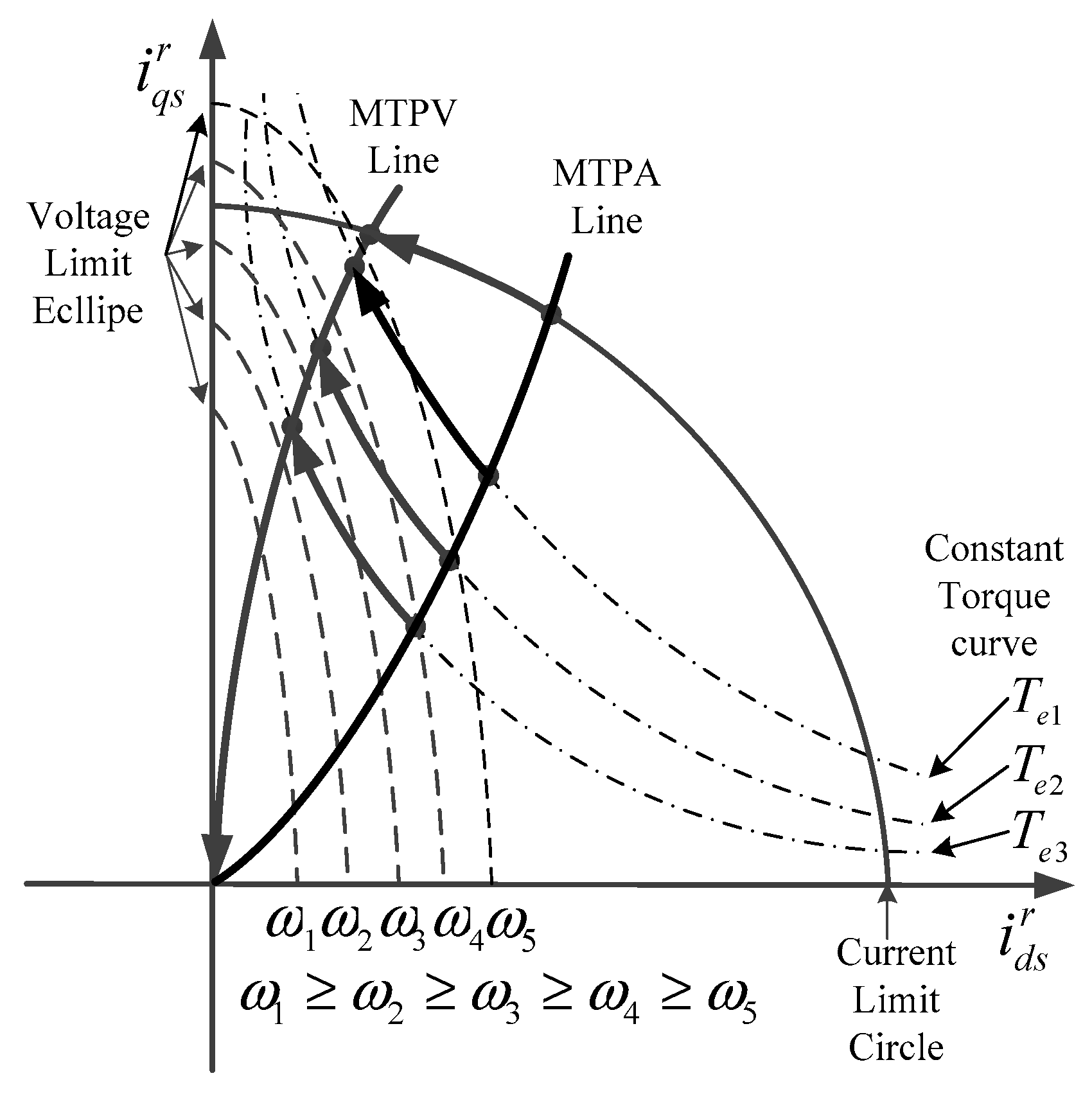
This paper proposes a flux weakening method based on current reference modification. The proposed method modifies the operating point in real time. The determination of the operating point movement is based on the information of the voltages and currents at the operating point. The direction and magnitude of the movement are calculated, and the point follows the SynRM current trajectory, as shown in Figure 1. Therefore, the proposed method does not require any tables to achieve the flux weakening control. The flux weakening performance can be improved by the flux saturation model. There is no additional procedure to generate tables for the flux weakening control in the conventional methods. The proposed method utilizes the voltage and current information on the operating point, so that the accuracy can be kept.

In Section 2, the flux saturation model of this paper is described. Section 3 contains a description of the proposed flux weakening algorithm. In Section 4, the results of the proposed algorithm, tested on a 3 kW SynRM, are presented. Section 5 concludes this paper.

2. SynRM Model

2.1. Basic Equation

In a rotor reference frame, the stator voltage equations are given by

$$\begin{array}{l}{V}_{ds}^r=R_s{i}_{ds}^r+\frac{d{\lambda }_{ds}^r}{dt}-{\omega }_r{\lambda }_{qs}^r\\ V_{qs}^r=R_s{i}_{qs}^r+\frac{d{\lambda }_{qs}^r}{dt}+{\omega }_r{\lambda }_{ds}^r\end{array}$$

(1)

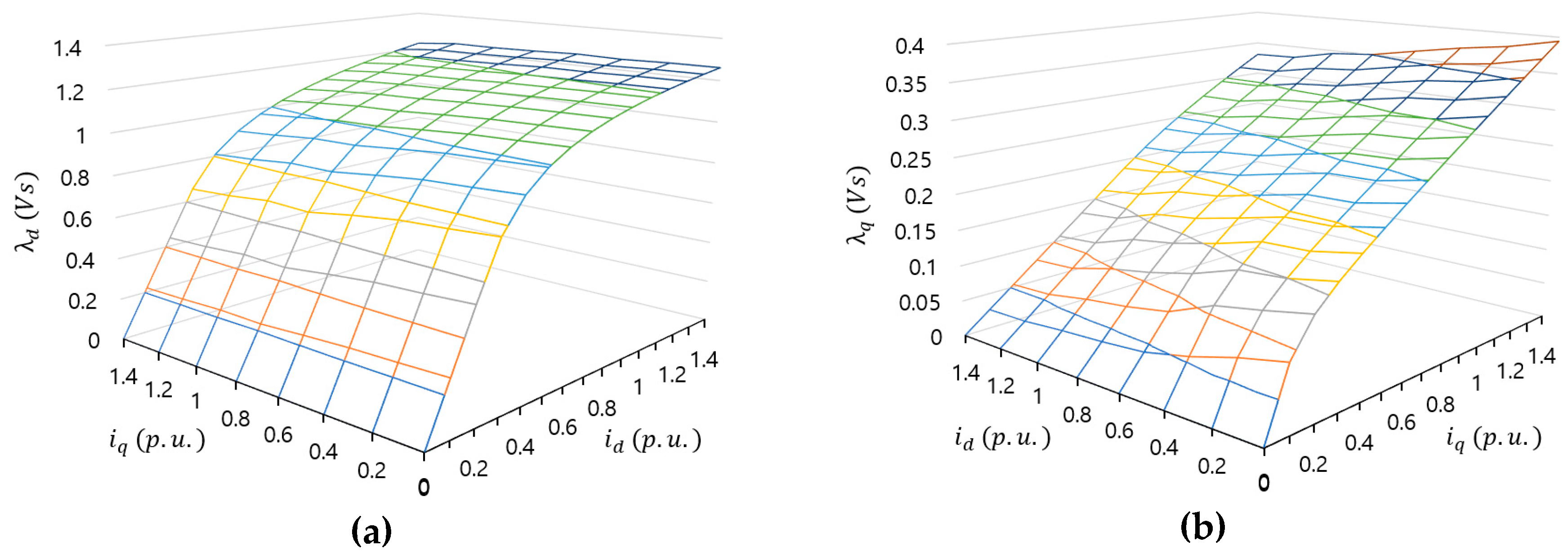
where ${\mathrm{V}}_{\mathrm{ds}}^{\mathrm{r}}$ and ${\mathrm{V}}_{\mathrm{qs}}^{\mathrm{r}}$ are the d-q axis voltages; $R_s$ is the stator resistance; $i_{ds}^r$ and $i_{qs}^r$ are the d-q axis currents; and ${\omega }_r$ is the electrical angular velocity. The d-q axis fluxes, ${\lambda }_{ds}^r$ and ${\lambda }_{qs}^r$, are nonlinear functions of $i_{ds}^r$ and $i_{qs}^r$, as shown in Figure 2. The torque equation is given by

$$T_e=\frac{3}{2}\frac{P}{2}\left({\lambda }_{ds}^r(i_{ds}^r,i_{qs}^r)·i_{qs}^r-{\lambda }_{qs}^r(i_{ds}^r,i_{qs}^r)·i_{ds}^r\right)$$

(2)

where P represents the poles of the motor.

2.2. Flux Saturation Model

To accurately operate flux weakening, the flux saturation characteristics of SynRMs should be considered. A standstill self-identification method [18] can be used to obtain the flux model. The d-axis flux saturation model is given by Equation (3). Depending on the magnitude of the current, it is divided into two areas:

$${\lambda }_d(I_d)=\{\begin{array}{ll}{L}_{0d}·I_d& for\left|I_d\right|<I_{thr}\\ sign(I_d){\lambda }_{0d}+L_{1d}{I}_d+\frac{{\beta }_d}{I_d}& for\left|I_d\right|\ge I_{thr}\end{array}$$

(3)

where $I_d$ is the d-axis current; ${\lambda }_d$ is the d-axis flux; $L_{0d}$ is the inductance in a linear region; and ${\lambda }_{0d}$, $L_{1d}$, and ${\beta }_{\mathrm{d}}$ are the constant weight coefficients in a saturation region.

The coefficients of Equation (3) are estimated using Multiple Linear Regression (MLR). At $I_{\mathrm{thr}}$, the dynamic inductances $L_{\mathrm{dyna}}$ and apparent inductances $L_{\mathrm{app}}$ in the saturation region are equal [18]. This is expressed as

$$L_{d,app}(I_{thr})=L_{d,dyna}(I_{thr})for\left|I\right|\ge I_{thr}.$$

(4)

Using Equation (3), Equation (4) is expressed as

$$\frac{{\lambda }_0}{I_{thr}}+L_1+\frac{\beta }{I_{thr}^2}=L_1-\frac{\beta }{I_{thr}^2}for\left|I\right|\ge I_{thr}.$$

(5)

${\mathrm{I}}_{\mathrm{thr}}$ is expressed as

$$I_{thr}=-\frac{2\beta }{{\lambda }_0}.$$

(6)

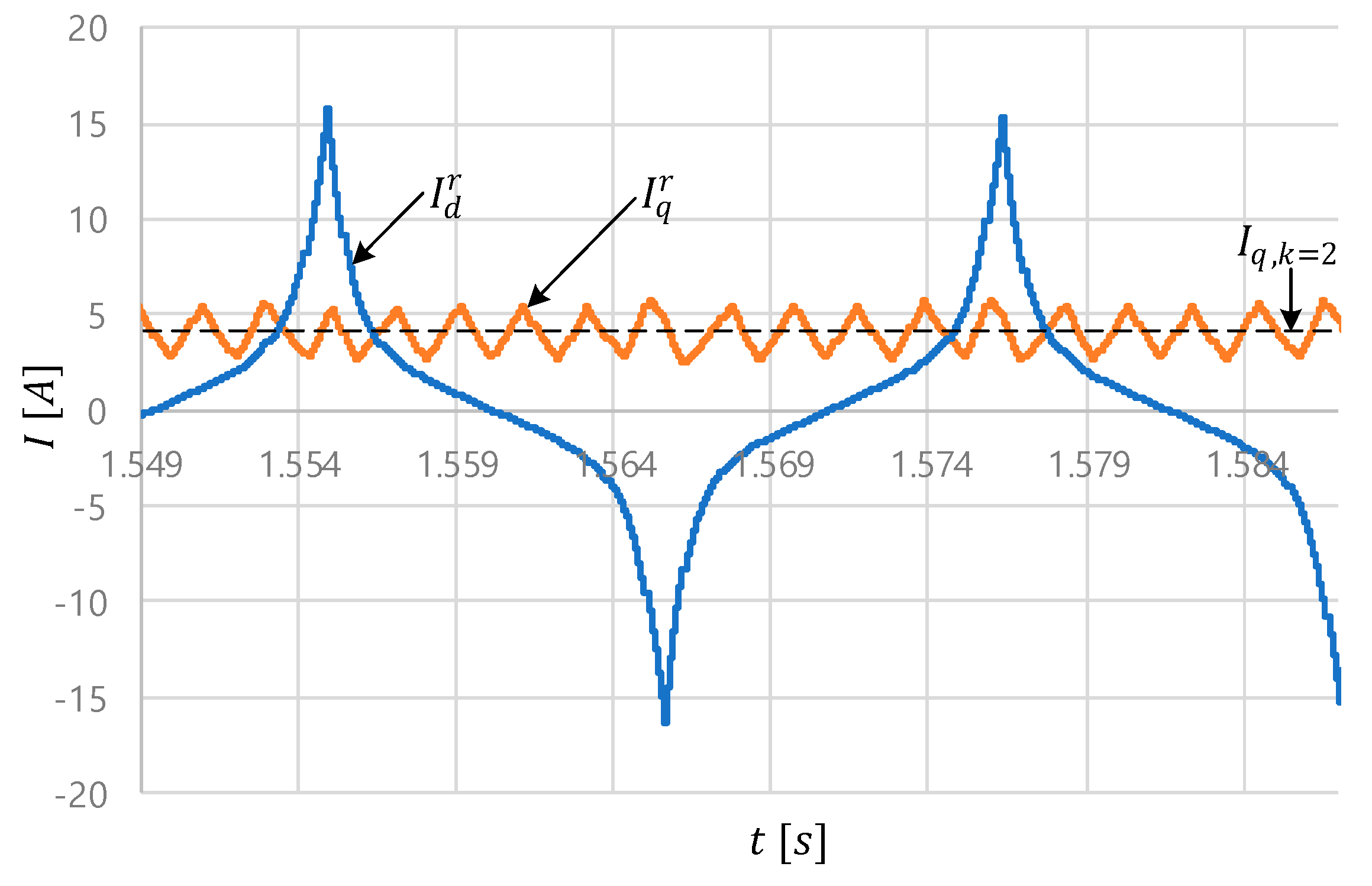
The flux saturation model is identified under the various q-axis currents in order to consider the cross-coupling effect. This paper used the flux saturation model [18]. The flux saturation model does not include cross-coupling terms. So, the flux saturation models were estimated considering the magnitude of the q-axis current. The hysteresis control was used to control the currents. Figure 3 shows the d-q axis current waveform to estimate the d-axis flux saturation model with ${\mathrm{I}}_{\mathrm{q},\mathrm{k}}$ of k = 2 and M = 5.

The magnitude of the q-axis current is selected as

$$I_{q,k}=(I_{rated}/M)·k,k=0,1,\cdots ,K$$

(7)

where $M$ determines the equally spaced magnitudes of the q-axis current, i.e., M = 5, and $k$ determines the magnitude of the q-axis current. $K$ denotes the maximum magnitude of the q-axis current during the identification of the d-axis flux model. As a result, the d-axis flux saturation models of the q-axis current are obtained. The d-axis flux function of $I_d$ with the q-axis current of is expressed as

$${{\lambda }_d(I_d)|}_{I_{q,k}}=\{\begin{array}{ll}{L}_{0d,k}·I_d& for\left|I_d\right|<I_{thr,k}\\ sign(I_d)·{\lambda }_{0d,k}+L_{1d,k}·I_d+\frac{{\beta }_{d,k}}{I_d}& for\left|I_d\right|\ge I_{thr,k}\end{array}.$$

(8)

Figure 2a shows the results of Equation (8). Using the interpolation method, the d-axis flux for the operating point can be calculated by

$${\lambda }_d(I_{d0},I_{q0})=\frac{{{\lambda }_d(I_{d0})|}_{I_{q,k+1}}-{{\lambda }_d(I_{d0})|}_{I_{q,k}}}{I_{q,k+1}-I_{q,k}}·(I_{q0}-I_{q,k})+{{\lambda }_d(I_{d0})|}_{I_{q,k}},\mathrm{for}{I}_{q,k}\le I_{q0}<I_{q,k+1}.$$

(9)

The quantities at the operating point are marked with the subscript 0. Similarly, the q-axis flux model can be obtained.

The apparent and dynamic inductances at the operating point can be calculated from the flux saturation model of Equation (8). The apparent inductance is expressed as

$${L_{app,d}|}_{I_{d0},I_{q0}}\equiv \frac{\lambda }{I}=\frac{{\lambda }_d(I_{d0},I_{q0})}{I_{d0}}.$$

(10)

The dynamic inductance is expressed as

$${L_{dyna,d}|}_{I_{d0},I_{q0}}\equiv \frac{\partial \lambda }{\partial I}={\frac{\partial {\lambda }_d(I_d,I_{q0})}{\partial I_d}|}_{I_{d0}}.$$

(11)

3. Proposed Flux Weakening Control Algorithm

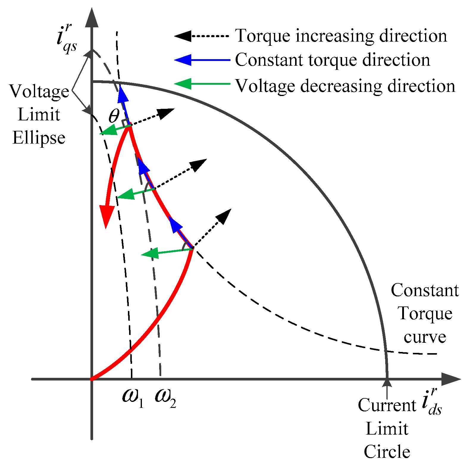
The operation trajectory of the SynRM is shown in Figure 4. The operating points in the constant torque region are on the maximum torque per ampere (MTPA) line. As the speed increases, the magnitude of the voltage limit curve decreases. The operating point moves along a constant torque curve to satisfy the voltage limitation. The area of the flux weakening operation along the constant torque curve is called the flux weakening region one (FWR1). As the speed increases further, the torque cannot be maintained in the FWR1 due to the voltage limitation. Therefore, the magnitude of the torque decreases, and the voltage limitation is satisfied. This operating point moves along the maximum torque per voltage (MTPV) curve. This region is called the flux weakening region two (FWR2). At the transition from FWR1 to FWR2, the constant torque and voltage limit curves meet at a point. The flux weakening region at the operating point is determined by the angle between the direction vectors of the curves.

3.1. Determination of Directions

Figure 4 shows the direction of the SynRM flux weakening. The flux weakening region is determined by the angle, θ, between the constant torque and voltage decreasing directions. If the angle is less than 90°, the operating point moves along the constant torque curve. If the angle is greater than 90°, it moves along the MTPV curve due to the voltage limitation. The operating region changes from FWR1 to FWR2. The inner product of the constant torque and voltage decreasing directions is used to calculate the angle, θ.

3.1.1. Constant Torque Direction

The magnitude of the torque is constant in FWR1. The constant torque direction is obtained using a torque equation given by Equation (2). A partial derivative can be used to obtain the gradient of function. The gradient means the direction of fastest increase. The torque increasing direction is calculated using the partial derivative. Since the direction is expressed in the d-q current plane, the partial derivative of torque with respect to d-q currents was used. The torque increasing direction at the operating point is expressed as

$$\left(\frac{\partial T_e}{\partial i_{ds}^r},\frac{\partial T_e}{\partial i_{qs}^r}\right).$$

(12)

Since the constant torque direction is perpendicular to the torque increasing direction, the constant torque direction is derived from the torque increasing direction as

$$(X_d,X_q)\equiv \left(-\frac{\partial T_e}{\partial i_{qs}^r},\frac{\partial T_e}{\partial i_{ds}^r}\right).$$

(13)

The magnitude is given by

$$X=\sqrt{X_d{}^2+X_q{}^2}.$$

(14)

3.1.2. Voltage Decreasing Direction

The voltage decreasing direction was obtained by the gradient descent method [30]. The cost function is expressed as

$$J=\frac{1}{2}\left\{{\left(V_{ds}^r\right)}^2+{\left(V_{qs}^r\right)}^2\right\}.$$

(15)

On the flux weakening region, the motor voltage is high, and the voltage drop on the stator resistance is relatively low compared to the motor voltage. So, the voltage drop on the stator resistance can be neglected. At the steady state, the output voltages on the d-q axis are given by

$$V_{ds}^r\approx -{\omega }_r·{\lambda }_{qs}^r(i_{ds}^r,i_{qs}^r),V_{qs}^r\approx {\omega }_r·{\lambda }_{ds}^r(i_{ds}^r,i_{qs}^r).$$

(16)

The direction vector, which reduces the magnitude of the output voltage, and its magnitude are given by Equation (17) and (18), respectively.

$$\left(Y_d,Y_q\right)\equiv -\nabla J=-\left(\frac{\partial J}{\partial i_{ds}^r},\frac{\partial J}{\partial i_{qs}^r}\right),$$

(17)

$$Y=\sqrt{Y_d{}^2+Y_q{}^2}.$$

(18)

Using Equation (13) and (17), θ is given by

$$\cos \theta =\frac{\left(X_d,X_q\right)·\left(Y_d,Y_q\right)}{X·Y}.$$

(19)

The flux weakening region can be determined by Equation (19) at the operating point. If θ is greater than 90°, the region is in FWR2. In FWR2, the operating point should be moved along the MTPV direction.

3.1.3. MTPV Direction

The MTPV condition is satisfied at the point where the voltage limit ellipse meets the constant torque curve. The condition is described by

$$\frac{\partial T_e}{\partial i_{ds}^r}·\frac{\partial V_{mag}^2}{\partial i_{qs}^r}-\frac{\partial T_e}{\partial i_{qs}^r}·\frac{\partial V_{mag}^2}{\partial i_{ds}^r}=0$$

(20)

where ${\mathrm{V}}_{\mathrm{mag}}$ is the magnitude of the output voltage. It is expressed as

$$V_{mag}=\sqrt{{\left(V_{ds}^{r*}\right)}^2+{\left(V_{qs}^{r*}\right)}^2}.$$

(21)

In FWR2, the current trajectory moves along the MTPV lines, and the operating point moves toward the origin, as shown in Figure 3. The d-axis current under the MTPV condition is small, so the d-axis flux is in the linear region, and the q-axis flux is almost linear. It could be considered that the d-q axis flux is a linear function in FWR2 for simplicity. The MTPV condition can be simplified as

$${\lambda }_{qs}^r(i_{qs}^r,i_{ds}^r)-{\lambda }_{ds}^r(i_{ds}^r,i_{qs}^r)=0.$$

(22)

To calculate the direction of the MTPV, the MTPV condition, $f_{MPTV}$, is defined as

$$f_{MTPV}\equiv {\lambda }_{qs}^r(i_{qs}^r,i_{ds}^r)-{\lambda }_{ds}^r(i_{ds}^r,i_{qs}^r).$$

(23)

The direction vector for increasing $f_{MPTV}$ is expressed as

$$\left(\frac{\partial f_{MTPV}}{\partial i_{ds}^r},\frac{\partial f_{MTPV}}{\partial i_{qs}^r}\right).$$

(24)

The direction vector for increasing $f_{MTPV}$ is perpendicular to the tangential direction vector of $f_{MTPV}$, which is the MTPV direction. Therefore, the MTPV direction and its magnitude are expressed by Equation (25) and (26), respectively.

$$(W_d,W_q)\equiv \left(-\frac{\partial f_{MTPV}}{\partial i_{qs}^r},\frac{\partial f_{MTPV}}{\partial i_{ds}^r}\right)$$

(25)

$$W=\sqrt{W_d{}^2+W_q{}^2}$$

(26)

For simplicity, the direction vector can be calculated using the apparent inductance, rather than the dynamic inductance. In this case, the flux is given by the product of the inductance and current, and the partial derivative of the flux to the current is equal to the apparent inductance of Equation (10). Therefore, the direction vectors can be calculated using Equation (10).

However, for a precise flux weakening operation, the dynamic inductance can be utilized in order to calculate the direction vector with consideration of the dynamic inductance, and the direction vectors can be calculated using Equation (11).

3.2. Determination of the Magnitude of a Change for Reference Modification

To implement the flux weakening operation, the operating point must be moved in accordance with the output voltage. The operating point of the current is moved with the error of the output voltage. The error of the output voltage is given by

$$\Delta V=V_{mag}-\frac{V_{dc}}{\sqrt{3}}·\eta$$

(27)

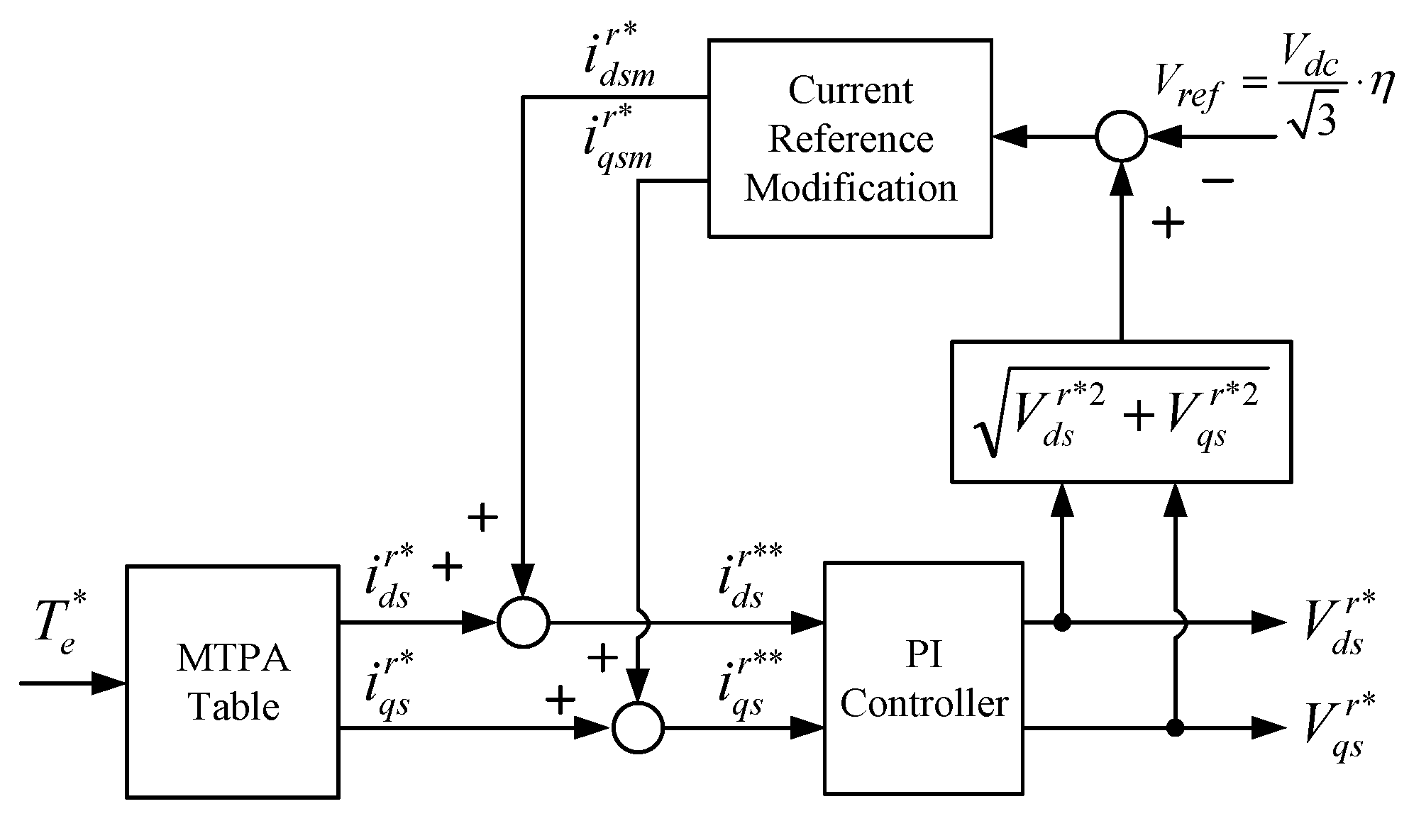
where $V_{dc}$ is the DC link voltage and $\eta$ is the voltage margin for the current controller. For the output voltage magnitude limitation, the current references should be modified from the current references $i_{ds}^{r^{*}}$ and $i_{qs}^{r^{*}}$ obtained from the MTPA table. The modified current references, $i_{ds}^{r^{**}}$ and $i_{qs}^{r^{**}}$, can be expressed as

$$i_{ds}^{r**}=i_{ds}^{r*}+i_{dsm}^{r*},i_{qs}^{r**}=i_{qs}^{r*}+i_{qsm}^{r*}.$$

(28)

The modification of the currents, $i_{dsm}^{r^{*}}$ and $i_{qsm}^{r^{*}}$, can be obtained in the form of integrals;

$$i_{dsm}^{r*}={\displaystyle \int M_{d}dt},i_{qsm}^{r*}={\displaystyle \int M_{q}dt}$$

(29)

where $M_d$ and $M_q$ are the magnitudes of a change, which indicate a direction and its magnitude for the modification of the current references. These can be calculated by the direction of the modified current reference and magnitude of the output voltage error according to the flux weakening region:

$$M_d=\{\begin{array}{l}{\alpha }_1·\Delta V·\frac{X_d}{X},\mathrm{in}\mathrm{the}\mathrm{FWR}1\\ {\alpha }_2·\Delta V·\frac{W_d}{W},\mathrm{in}\mathrm{the}\mathrm{FWR}2\end{array}$$

(30)

$$M_q=\{\begin{array}{l}{\alpha }_1·\Delta V·\frac{X_q}{X},\mathrm{in}\mathrm{the}\mathrm{FWR}1\\ {\alpha }_2·\Delta V·\frac{W_q}{W},\mathrm{in}\mathrm{the}\mathrm{FWR}2\end{array}$$

(31)

where ${\alpha }_1$ and ${\alpha }_2$ are the reference modification gains of FWR1 and FWR2, respectively. When the output voltage is not saturated, this algorithm does not operate, and $i_{dsm}^{r^{*}}$ and $i_{qsm}^{r^{*}}$ are set to zero.

The block diagram of the proposed algorithm is shown in Figure 5. The MTPA table was made by searching the operating points where the maximum torque is generated among the currents that have the same magnitude. The cross-saturation flux model was used for making the MTPA table.

4. Simulations and Experiments

4.1. Experimental Equipment and Conditions

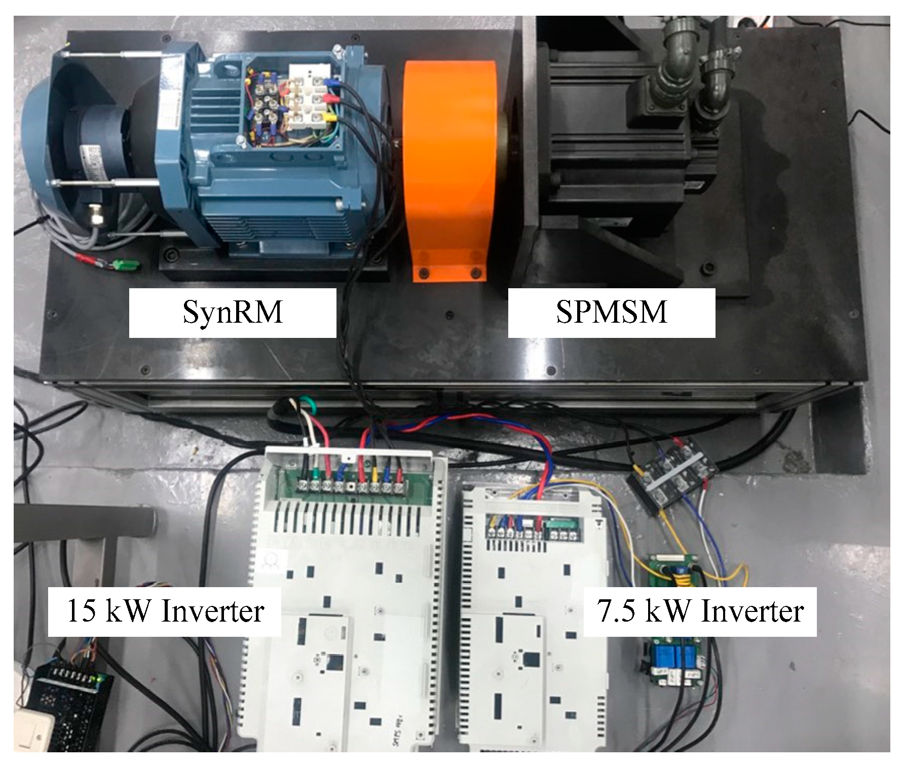
Experiments were performed using a M-G set consisting of a 3 kW SynRM and 5 kW surface-mounted permanent magnet synchronous motor (SPMSM), as shown in Figure 6. Two 7.5 kW and 15 kW inverters were used to drive the SynRM and SPMSM, respectively.

Table 1. Nominal parameters of the 3 kW SynRM.

Nominal Parameter	Value [unit]
Rated power	3.0 [kW]
Rated speed	1500 [r/min]
Number of poles	4
Rated voltage	400 [${\mathrm{V}}_{\mathrm{rms}}$]
Rated current	7 [${\mathrm{A}}_{\mathrm{rms}}$]
Stator resistance	1.9059 [Ω]
d-axis inductance	220 [mH]
q-axis inductance	40 [mH]

provides the nominal parameters of the tested SynRM. The DC link voltage of the inverters for the motor drive was 530 V, with a switching frequency of 5 kHz. The inverters were fed by the space vector pulse width modulation (SVPWM).

The performances of the proposed flux weakening algorithm on FWR1 and FWR2 were tested. The SPMSM was controlled by a speed controller. The SynRM was controlled by a torque controller with the flux weakening operation. The saturation characteristics of the SynRMs were considered in the current controller, which uses a model-based current controller [22]. The bandwidth of the current controller was 200 Hz.

The d-q axis flux saturation models were identified up to the 1.4 p.u. d-q axis currents based on the standstill self-identification method [18]. For the calculation of Equation (7), M = 5 and K = 7. When k = 0 in Equation (8), the flux model becomes a self-axis flux saturation model. When k is not zero, the flux model is under cross-coupling effects. The identification results are shown in Figure 2. Extrapolation can be used if the current operating point is outside the measured range.

Generally, SynRMs are designed for operation up to FWR1. However, to verify the feasibility of the proposed flux weakening algorithm up to FWR2, simulations and experiments were performed under the limitation of only 40% of the DC link voltage by setting $\mathsf{\eta }=0.4$. The voltage reference in Figure 4, V_ref, was set to 212 V. The reference modification gains ${\alpha }_1$ and ${\alpha }_2$ were set to ${\mathsf{\omega }}_{\mathrm{r}}/40$.

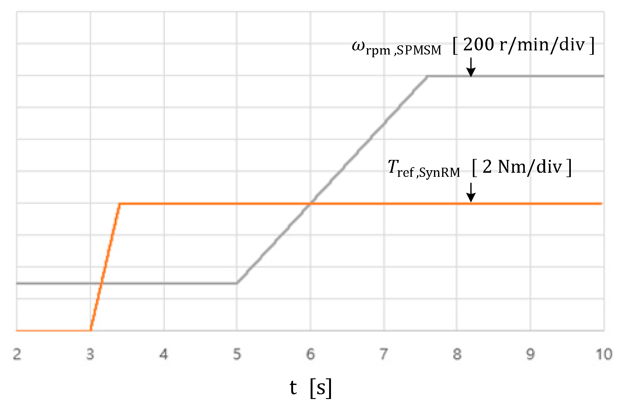
Figure 7 shows an experimental sequence to verify the proposed algorithm. SPMSM controlled the speed, and the initial speed was 300 r/min. Then, the torque reference of SynRM was increased to 8 Nm. Thereafter, the speed was increased to 1600 r/min. As the speed increases, the output voltages are saturated, and the flux weakening control was performed. According to the speed, the output torque will decrease.

The flux saturation characteristics of the simulation motor were set similarly, considering the flux saturation characteristics of Figure 2. The operating conditions of the simulations are the same as the operating conditions of the experiments.

4.2. Results and Discussion

To verify the performance of the algorithm, the operating point of the current, and the torque according to a change in the speed, were checked. The torque was obtained by the output of the speed controller of the SPMSM. Three cases were tested to evaluate the flux weakening performance with respect to the accuracy of the flux model:

• using the apparent inductance of the self-axis flux saturation model,
• using the dynamic inductance of the self-axis flux saturation model, and
• using the dynamic inductance of the cross-coupled flux saturation model.

The first case is simple, and the flux weakening algorithm is easily implemented. The third case is the most complex, because the dynamic inductance is calculated during the flux weakening operation. The simulation results for each case are shown in Figure 8, Figure 9 and Figure 10. Their trajectories are demonstrated in Figure 11. The experimental results for each case are shown in Figure 12, Figure 13 and Figure 14. Their trajectories of experiments are in Figure 15.

4.2.1. Simulations

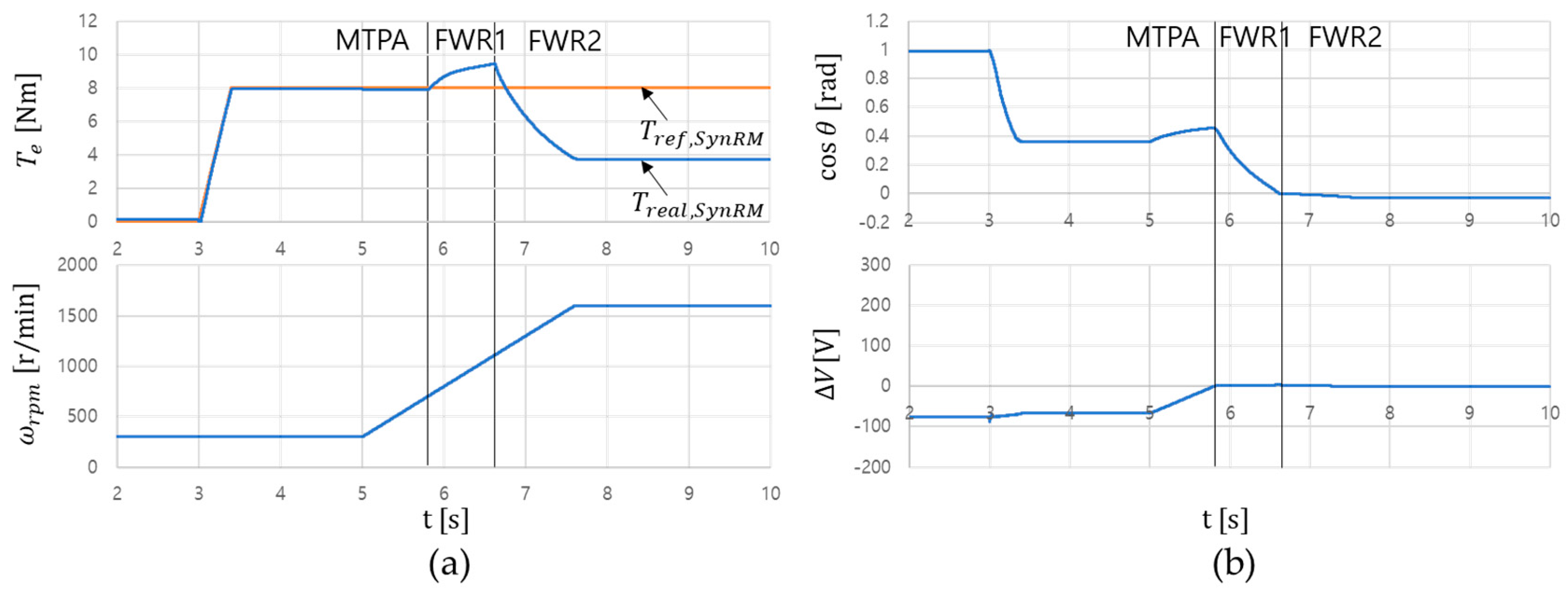
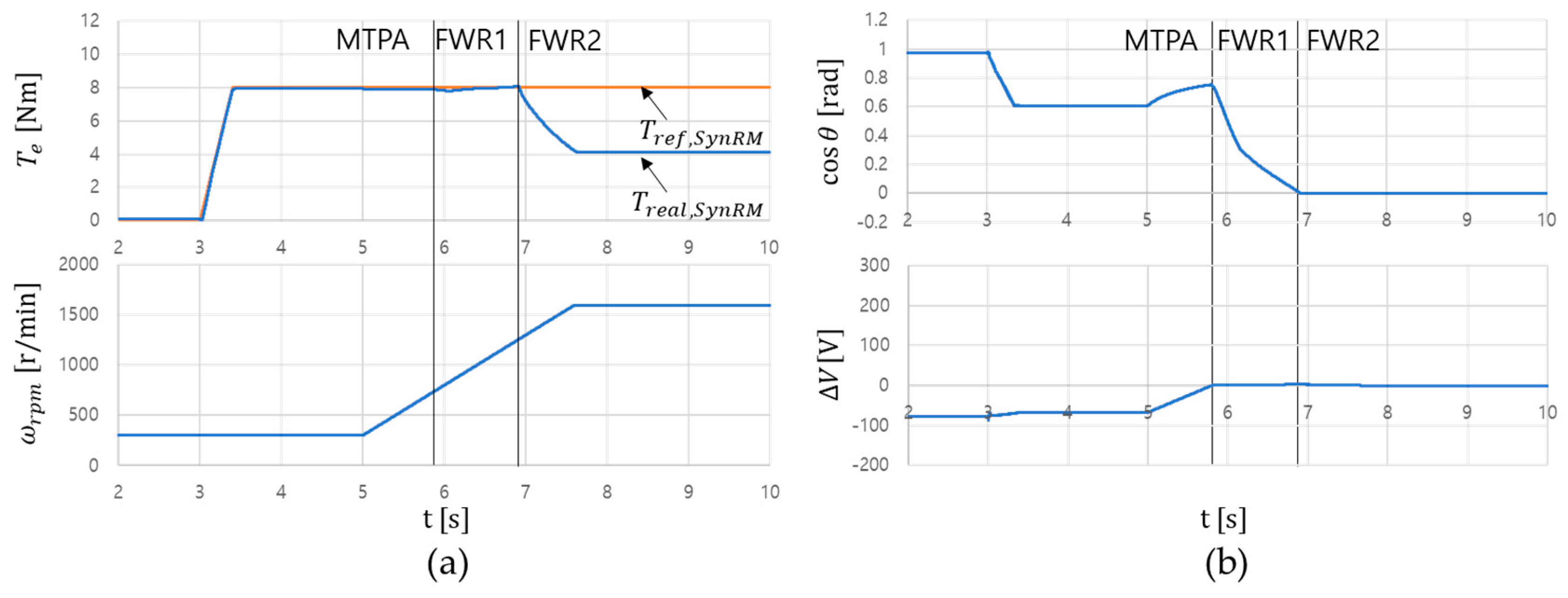
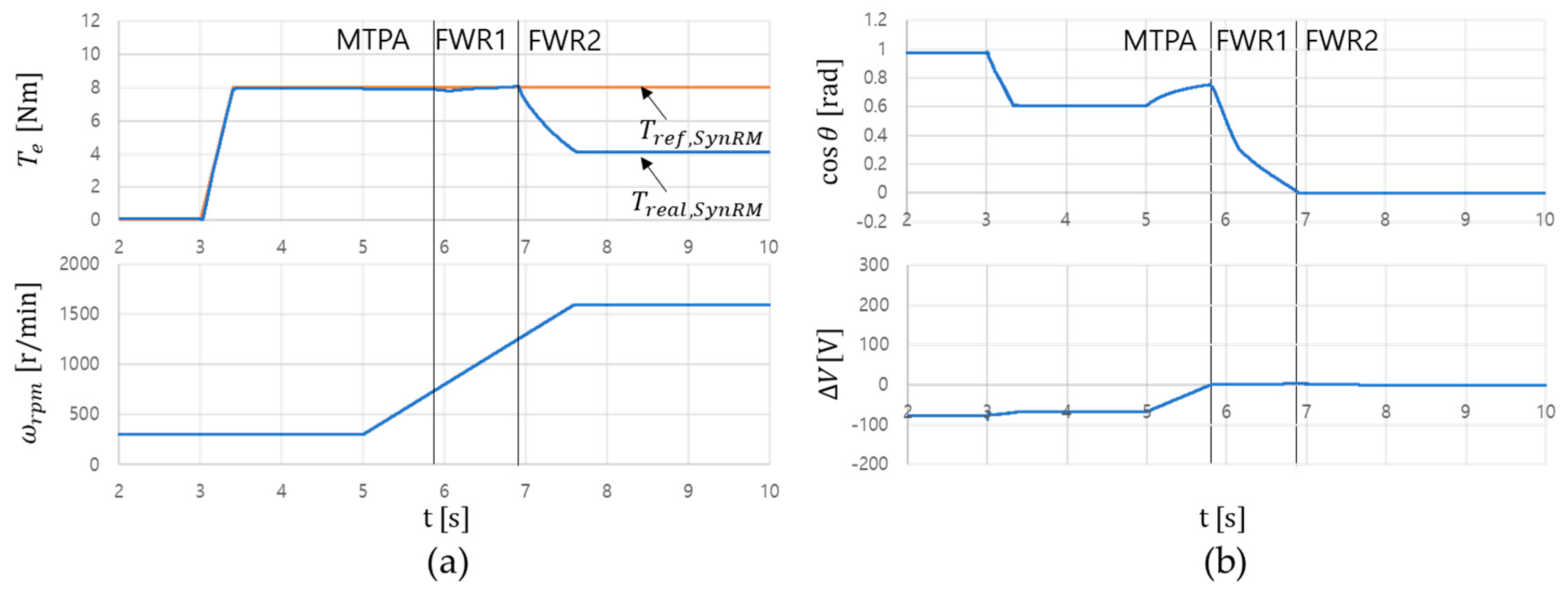
Figure 8, Figure 9 and Figure 10 show the simulation results for the three cases. Figure 8a, Figure 9a, and Figure 10a show the speed and torque of the SynRM. The torque reference and real torque of the SynRM are demonstrated. In Figure 8a, the real torque was increased as speed increased in FWR1. On the other hand, Figure 9a and Figure 10a show different waveforms. The real torque is maintained in FWR1. From the waveforms, the use of the apparent inductance degrades the flux weakening performance.

Figure 8b shows cosθ and ∆V in the proposed method. The operating point moved from the MTPA line to the FWR1 when ∆V approached zero. As the speed increased further, cosθ approached zero. After that, the operating point moved from FWR1 to the FWR2. As explained before, the proposed method worked well.

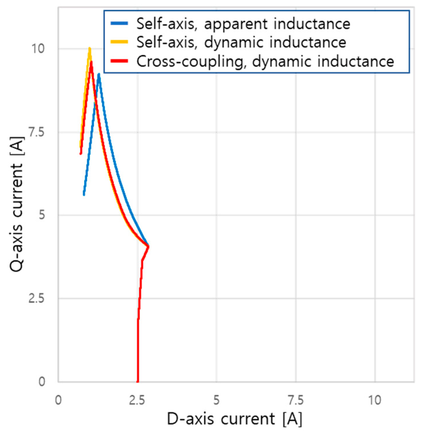
Figure 11 shows the current trajectory for three cases. The blue, yellow, and red lines represent the results of Figure 8, Figure 9 and Figure 10, respectively. By comparing the blue line with the others, it can be seen that the trajectory obtained using the dynamic inductance of the flux model differs greatly from that obtained using the apparent inductance. Detailed explanations and the discussion will be addressed with experiments.

4.2.2. Experiments

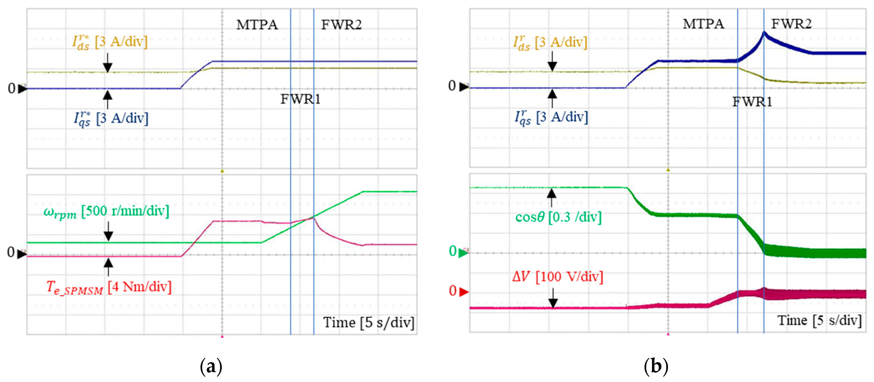
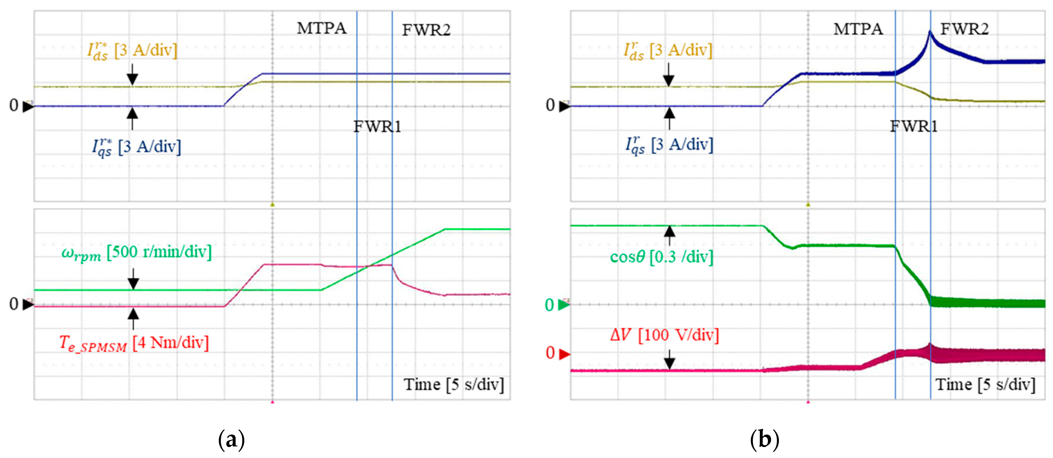
Figure 12 shows the experimental results for the first case. Figure 12a shows the current references from the MTPA table ($i_{ds}^{r^{*}}$ and $i_{qs}^{r^{*}}$), as well as the speed and torque of the SPMSM. The MTPA table was determined using the identified flux model performed before the experiments. Figure 12b shows the d-q axis currents, $\cos \theta$, and $\Delta V$. The d-q axis currents were regulated as the modified currents, $i_{ds}^{r^{**}}$ and $i_{qs}^{r^{**}}$. These were modified from the current references from the MTPA tables, $i_{ds}^{r^{*}}$ and $i_{qs}^{r^{*}}$. The differences between the real currents and those from the MTPA tables provide the modifications of the currents, $i_{dsm}^{r^{*}}$ and $i_{qsm}^{r^{*}}$.

During the operation on the MTPA line, the real currents were equal to the current references from the MTPA table, $i_{ds}^{r^{*}}$ and $i_{qs}^{r^{*}}$. As the speed increased, $\Delta V$ approached zero. When $\Delta V$ became zero, the operating point transitioned from the MTPA line to FWR1, as shown in Figure 12b. As the speed increased further, $\cos \theta$ approached zero. When $\cos \theta$ became zero, the operating point transitioned from FWR1 to FWR2. During the flux weakening operation from the MTPA line to FWR2, the current references from the MTPA table remained constant. Therefore, the proposed method worked well. However, as shown in Figure 12a, during the operation on FWR1, the torque of the SPMSM increased. Since the operating point on FWR1 should move along the constant torque line, the trajectory of the currents on FWR1 was not exact. This inaccuracy may be due to the use of the apparent inductance for the flux weakening algorithm. For the first case, the direction vectors were calculated using the apparent inductance of the self-axis flux saturation model.

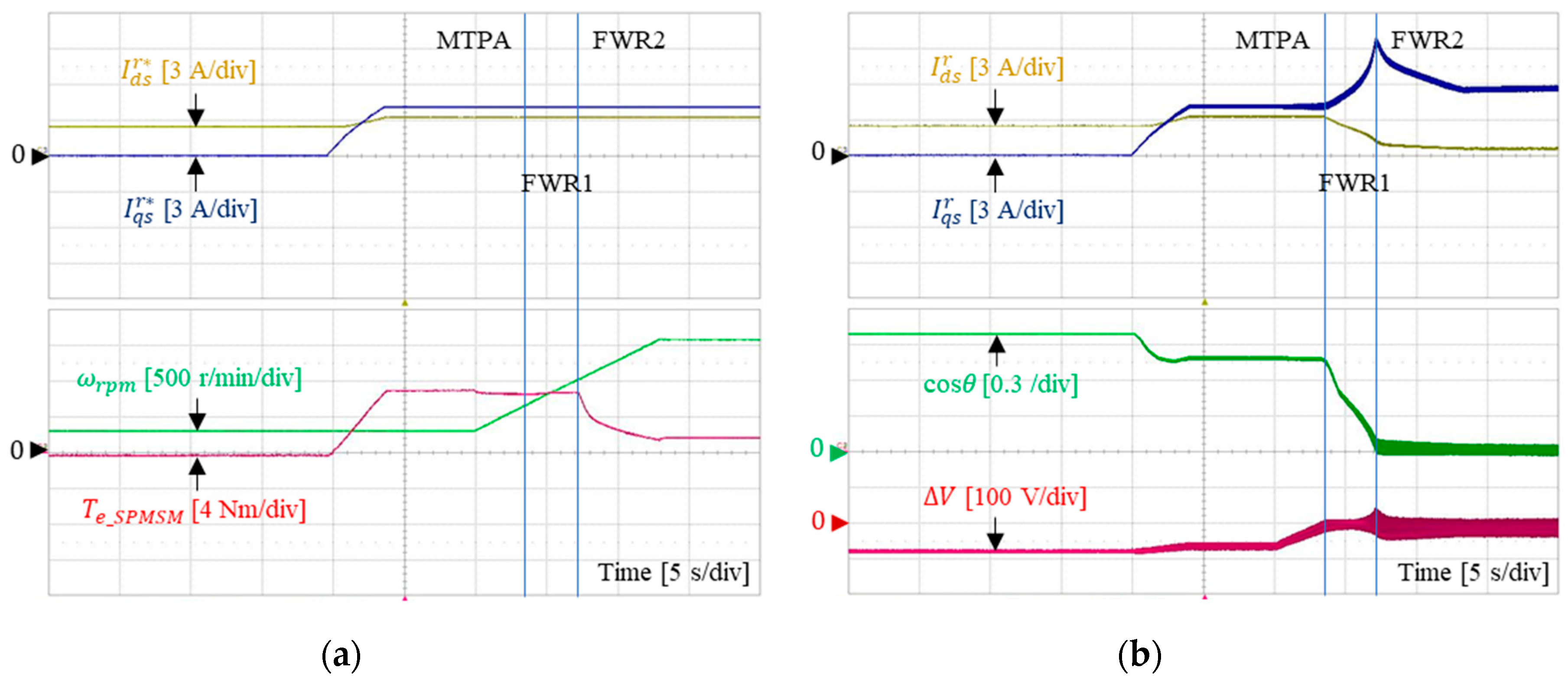
The waveforms of Figure 13 and Figure 14 are the same of those of Figure 12. The only difference between the methods used to obtain these curves were the calculation methods of $\partial \lambda /\partial I$, which is the variation of the flux with respect to the current. For Figure 13, the direction vectors were calculated using the dynamic inductance of the self-axis flux saturation model, whereas for Figure 14, the same calculation was performed using the dynamic inductance of the cross-coupled flux model.

In Figure 13a, the torque in FWR1 is almost constant with a slight increase. The flux weakening operation shown in Figure 13 is more accurate than that shown in Figure 12. Figure 13b shows the flux weakening operation according to the magnitude of the voltage error and angle.

In Figure 14a, the torque in FWR1 is almost constant. Therefore, it can be concluded that the performance of the flux weakening algorithm for the case of Figure 14 was the best of the three experiments.

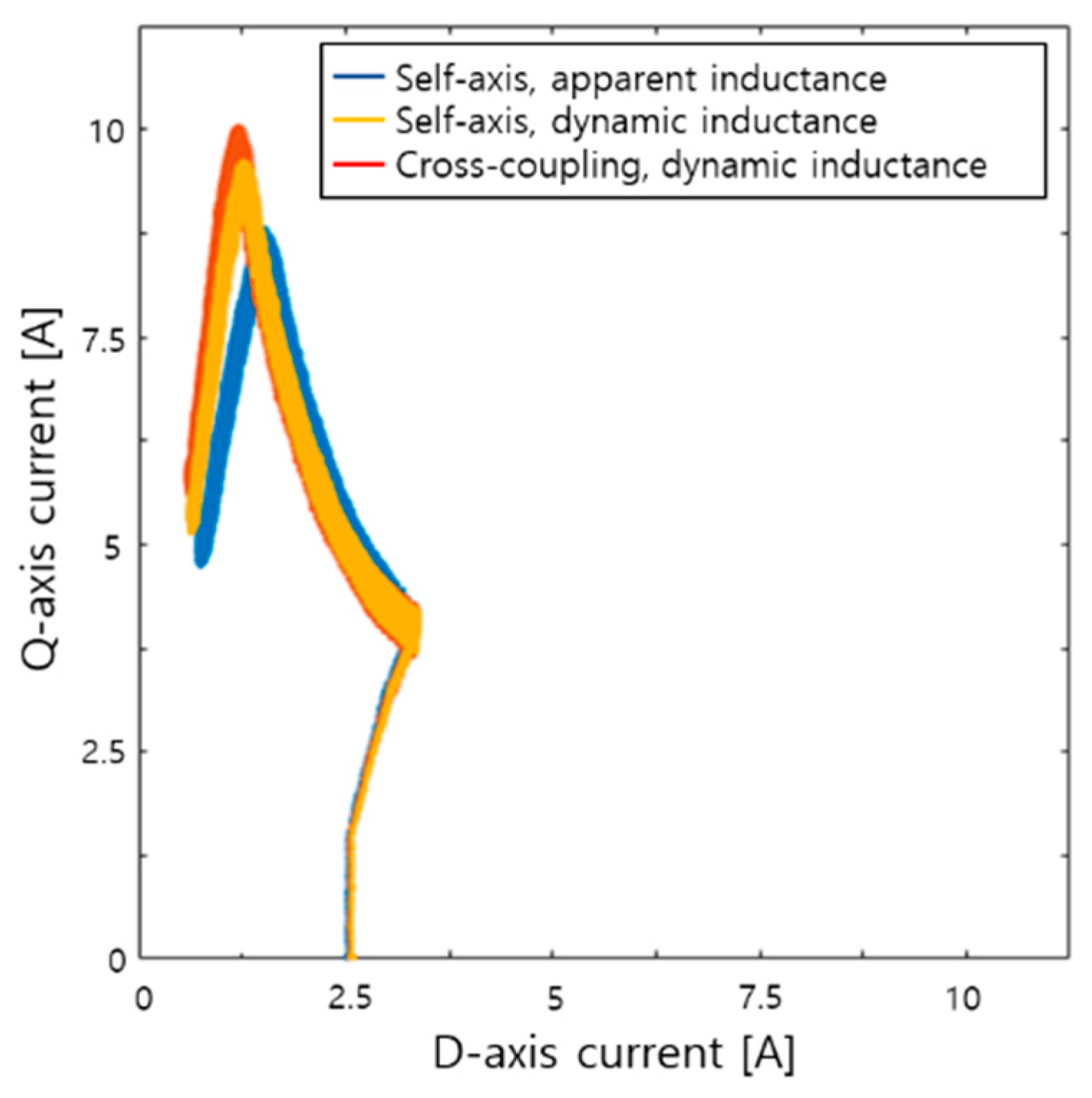
Figure 15 shows the trajectories of the currents in Figure 12, Figure 13 and Figure 14. The blue, yellow, and red lines represent the experimental results corresponding to Figure 12, Figure 13 and Figure 14, respectively. By comparing the blue line with the others, it can be seen that the trajectory obtained using the dynamic inductance of the flux model differs greatly from that obtained using the apparent inductance. From the figures, it can be seen that the use of accurate flux modeling is necessary for flux-saturated machines. Although the implementation of the flux weakening algorithm is complex, the flux weakening operation is precise when the dynamic inductance of the cross-coupled flux model is used.

5. Conclusions

This paper presents a flux weakening control algorithm using a flux saturation model that takes cross-coupling into account. The determination of a flux weakening region and the modification of current references were proposed. The flux weakening region is determined by the angle between direction vectors along the constant torque and voltage decreasing directions in the d-q axis current plane. After identifying the flux weakening region, the current references are modified for flux weakening according to the direction vector and appropriate magnitude. The direction and magnitude are determined by the operating point of the currents and magnitude of the output voltage, respectively.

Using the flux saturation model for SynRMs, the flux weakening direction can be determined accurately. As a result, flux weakening was performed without any tables. It is confirmed that accurate flux weakening control is possible by calculating the direction vectors and determining the operating region. Uses of apparent inductance and dynamic inductance were tested for the proposed method. To use the dynamic inductance obtained from the flux saturation model shows the best performance.

Compared to the conventional method based on the tables, the proposed method does not need the computation time to generate the tables, so that the initial commissioning process can be reduced. The simulations and experiments show that the algorithm is stable based on the modified current reference. The experimental results reveal the validity of the proposed algorithm, which can be applied to general-purpose inverters for high-speed SynRM drives.

References

- Boazzo, B.; Vagati, A.; Pellegrino, G.; Armando, E.; Guglielmi, P. Multipolar Ferrite-Assisted Synchronous Reluctance Machines: A General Design Approach. IEEE Trans. Ind. Electron. 2015, 62, 832–845. [Google Scholar] [CrossRef]
- Capolino, G.; Cavagnino, A. New Trends in Electrical Machines Technology—Part II. IEEE Trans. Ind. Electron. 2014, 61, 4931–4936. [Google Scholar] [CrossRef]
- Vagati, A. The synchronous reluctance solution: A new alternative in AC drives. In Proceedings of the IECON’94: 20th International Conference on Industrial Electronics, Control and Instrumentation, Bologna, Italy, 5–9 September 1994; pp. 1–13. [Google Scholar]
- Bianchi, N.; Bolognani, S. Magnetic models of saturated interior permanent magnet motors based on finite element analysis. In Proceedings of the 1998 IEEE Industry Applications Conference, St. Louis, MO, USA, 12–15 October 1998; pp. 27–34. [Google Scholar]
- Iwaji, Y.; Nakatsugawa, J.; Sakai, T.; Aoyagi, S.; Nagura, H. Motor drive system using nonlinear mathematical model for permanent magnet synchronous motors. In Proceedings of the 2014 International Power Electronics Conference (IPEC-Hiroshima 2014-ECCE ASIA), Hiroshima, Japan, 18–21 May 2014; pp. 2451–2456. [Google Scholar]
- Hinkkanen, M.; Pescetto, P.; Mölsä, E.; Saarakkala, S.E.; Pellegrino, G.; Bojoi, R. Sensorless Self-Commissioning of Synchronous Reluctance Motors at Standstill Without Rotor Locking. IEEE Trans. Ind. Appl. 2017, 53, 2120–2129. [Google Scholar] [CrossRef] [Green Version]
- Rahman, K.M.; Hiti, S. Identification of machine parameters of a synchronous motor. IEEE Trans. Ind. Appl. 2005, 41, 557–565. [Google Scholar] [CrossRef]
- Armando, E.; Bojoi, R.I.; Guglielmi, P.; Pellegrino, G.; Pastorelli, M. Experimental Identification of the Magnetic Model of Synchronous Machines. IEEE Trans. Ind. Appl. 2013, 49, 2116–2125. [Google Scholar] [CrossRef]
- Qu, Z.; Tuovinen, T.; Hinkkanen, M. Inclusion of magnetic saturation in dynamic models of synchronous reluctance motors. In Proceedings of the XXth International Conference on Electrical Machines (ICEM), Marseille, France, 2–5 September 2012; pp. 994–1000. [Google Scholar]
- Pellegrino, G.; Boazzo, B.; Jahns, T.M. Magnetic Model Self-Identification for PM Synchronous Machine Drives. IEEE Trans. Ind. Appl. 2015, 51, 2246–2254. [Google Scholar] [CrossRef] [Green Version]
- Odhano, S.A.; Bojoi, R.; Roşu, Ş.G.; Tenconi, A. Identification of the Magnetic Model of Permanent-Magnet Synchronous Machines Using DC-Biased Low-Frequency AC Signal Injection. IEEE Trans Ind. Appl. 2015, 51, 3208–3215. [Google Scholar] [CrossRef]
- Hanic, Z.; Vrazic, M.; Maljkovic, Z. Steady-state synchronous machine model which incorporates saturation and cross-magnetization effects. In Proceedings of the 2013 Fourth International Conference on Power Engineering, Energy and Electrical Drives (POWERENG), Istanbul, Turkey, 13–17 May 2013; pp. 1553–1557. [Google Scholar]
- Stumberger, B.; Stumberger, G.; Dolinar, D.; Hamler, A.; Trlep, M. Evaluation of saturation and cross-magnetization effects in interior permanent-magnet synchronous motor. IEEE Trans. Ind. Appl. 2003, 39, 1264–1271. [Google Scholar] [CrossRef]
- Kilthau, A.; Pacas, J.M. Parameter-measurement and control of the synchronous reluctance machine including cross saturation. In Proceedings of the 2001 IEEE Industry Applications Society 36th Annual Meeting—IAS’01, Chicago, IL, USA, 30 September–4 October 2001; pp. 2302–2309. [Google Scholar]
- Vagati, A.; Pastorelli, M.; Franceschini, G.; Drogoreanu, V. Flux-observer-based high-performance control of synchronous reluctance motors by including cross saturation. IEEE Trans. Ind. Appl. 1999, 35, 597–605. [Google Scholar] [CrossRef]
- Odhano, S.A.; Giangrande, P.; Bojoi, R.I.; Gerada, C. Self-Commissioning of Interior Permanent—Magnet Synchronous Motor Drives with High-Frequency Current Injection. IEEE Trans. Ind. Appl. 2014, 50, 3295–3303. [Google Scholar] [CrossRef]
- Awan, H.A.A.; Song, Z.; Saarakkala, S.E.; Hinkkanen, M. Optimal Torque Control of Saturated Synchronous Motors: Plug-and-Play Method. IEEE Trans. Ind. Appl. 2018, 54, 6110–6120. [Google Scholar] [CrossRef] [Green Version]
- Bedetti, N.; Calligaro, S.; Petrella, R. Stand-still self-identification of flux characteristics for synchronous reluctance machines using novel saturation approximating function and multiple linear regression. IEEE Trans. Ind. Appl. 2016, 52, 083–3092. [Google Scholar] [CrossRef]
- Bae, B.-H.; Sul, S.-K. A compensation method for time delay of full-digital synchronous frame current regulator of PWM AC drives. IEEE Trans. Ind. Appl. 2003, 39, 802–810. [Google Scholar] [CrossRef]
- Chang, S.-H.; Chen, P.-Y. Self-tuning gains of PI controllers for current control in a PMSM. In Proceedings of the 2010 5th IEEE Conference on Industrial Electronics and Applications, Taichung, Taiwan, 15–17 June 2010; pp. 1282–1286. [Google Scholar]
- Tursini, M.; Parasiliti, F.; Zhang, D. Real-time gain tuning of PI controllers for high-performance PMSM drives. IEEE Trans. Ind. Appl. 2002, 38, 1018–1026. [Google Scholar] [CrossRef]
- Awan, H.A.A.; Saarakkala, S.E.; Hinkkanen, M. Current Control of Saturated Synchronous Motors. In Proceedings of the Tenth Annual IEEE Energy Conversion Congress and Exposition (ECCE 2018), Portland, OR, USA, 23–27 September 2018; pp. 6953–6959. [Google Scholar]
- Hinkkanen, M.; Qu, Z.; Awan, H.A.A.; Tuovinen, T.; Briz, F. Current control for IPMSM drives: Direct discrete-time pole-placement design. In Proceedings of the 2015 IEEE Workshop on Electrical Machines Design, Control and Diagnosis (Wemdcd), Torino, Italy, 26–27 March 2015; pp. 156–164. [Google Scholar]
- Mansouri, B.; Piaton, J. Magnetic Saturation Aids Flux-Weakening Control: Using Lookup Tables Based on a Static Method of Identification for Nonlinear Permanent-Magnet Synchronous Motors. IEEE Electrification Magazine 2017, 5, 53–61. [Google Scholar] [CrossRef]
- Trancho, E.; Ibarra, E.; Arias, A.; Kortabarria, I.; Juergens, J.; Marengo, L.; Fricasse, A.; Gragger, J.V. PM-Assisted Synchronous Reluctance Machine Flux Weakening Control for EV and HEV Applications. IEEE Trans. Ind. Electron. 2018, 65, 2986–2995. [Google Scholar] [CrossRef] [Green Version]
- Lee, J.; Nam, K.; Choi, S.; Kwon, S. A Lookup Table Based Loss Minimizing Control for FCEV Permanent Magnet Synchronous Motors. In Proceedings of the 2007 IEEE Vehicle Power and Propulsion Conference (VPPC), Arlington, TX, USA, 9–12 September 2007; pp. 175–179. [Google Scholar]
- Bae, B.-H.; Patel, N.; Schulz, S.; Sul, S.-K. New field weakening technique for high saliency interior permanent magnet motor. In Proceedings of the 38th IAS Annual Meeting on Conference Record of the Industry Applications Conference, Salt Lake City, UT, USA, 12–16 October 2003; pp. 898–905. [Google Scholar]
- Awan, H.A.A.; Hinkkanen, M.; Bojoi, R.; Pellegrino, G. Stator-Flux-Oriented Control of Synchronous Motors: Design and Implementation. In Proceedings of the Tenth Annual IEEE Energy Conversion Congress and Exposition (ECCE 2018), Portland, OR, USA, 23–27 September 2018; pp. 6571–6577. [Google Scholar]
- Ferdous, S.M.; Garcia, P.; Oninda, M.A.M.; Hoque, M.A. MTPA and Field Weakening Control of Synchronous Reluctance motor. In Proceedings of the 9th International Conference on Electrical and Computer Engineering, Dhaka, Bangladesh, 20–22 December 2016; pp. 598–601. [Google Scholar]
- Ioannou, P.A.; Sun, J. Robust Adaptive Control; Prentice-Hall: Upper Saddle River, NJ, USA, 1996; pp. 785–786. [Google Scholar]
Figure 1.
Synchronous reluctance motor (SynRM) current trajectories.
Figure 2.
Flux linkages as functions of the currents including cross-coupling: (a) and (b) .
Figure 3.
Estimating the d-axis flux model with an of k = 2 and M = 5.
Figure 4.
Flux weakening directions of the SynRM.
Figure 5.
Block diagram of the proposed algorithm.
Figure 6.
Experimental test setup.
Figure 7.
Experimental sequence.
Figure 8.
Simulation results with the apparent inductance of the self-axis flux saturation model: (a) simulation conditions and (b) operation of the proposed algorithm.
Figure 9.
Simulation results with the dynamic inductance of the self-axis flux saturation model: (a) simulation conditions and (b) operation of the proposed algorithm.
Figure 10.
Simulation results with the dynamic inductance of the cross-coupled flux saturation model: (a) simulation conditions and (b) operation of the proposed algorithm.
Figure 11.
Results of comparing the operating points of the currents in Figure 8, Figure 9 and Figure 10.
Figure 12.
Experimental results with the apparent inductance of the self-axis flux saturation model: (a) maximum torque per ampere (MTPA) current reference and experimental conditions and (b) operation of the proposed algorithm.
Figure 13.
Experimental results with the dynamic inductance of the self-axis flux saturation model: (a) MTPA current reference and experimental conditions and (b) operation of the proposed algorithm.
Figure 14.
Experimental results with the dynamic inductance of the cross-coupled flux saturation model: (a) MTPA current reference and experimental conditions and (b) operation of the proposed algorithm.
Figure 15.
Results of comparing the operating points of the currents in Figure 12, Figure 13 and Figure 14.