Researching Why-Not Questions in Skyline Query Based on Orthogonal Range

Abstract

This paper aims to answer “why-not” questions in skyline queries based on the orthogonal query range (i.e., ORSQ). These queries retrieve skyline points within a rectangular query range, which improves query efficiency. Answering why-not questions in ORSQ can help users analyze query results and make decisions. We discuss the causes of why-not questions in ORSQ. Then, we outline how to modify the why-not point and the orthogonal query range so that the why-not point is included in the result of the skyline query based on the orthogonal range. When the why-not point is in the orthogonal range, we show how to modify the why-not point and narrow the orthogonal range. We also present how to expand the orthogonal range when the why-not point is not in the orthogonal range. We effectively combine query refinement and data modification techniques to produce meaningful answers. The experimental results demonstrate that the proposed algorithms have high-quality explanations for why-not questions in ORSQ in the real and synthetic datasets.

1. Introduction

In the past ten years, big data has received widespread attention. However, the data themselves have no value. After collection, storage [1], processing [2] and analysis, they generate value. For example, in intelligent communication systems, users use wireless sensors [3,4,5,6,7] and mobile devices to collect data, and then analyze the data to provide decision-making basis for programs. The wireless sensor is a type of wireless data communication collector which integrates data acquisition, data management, data communication and, other functions. In this paper, we will research a new problem, which is related to data analysis.

With the development of information technology, the performance of the database has been continuously improved. Many issues, such as privacy protection [8] and fault detection [9], have made great progress. However, the current database is still imperfect, and availability is one of the key points to refine the database. In the research of improving database usability, the “Why-Not” questions [10] have received more and more attention. In ordinary queries, users do not know the specific execution process of the query. When users find that the query results do not have the information they want, they often feel confused or even frustrated. The why-not question can explain to users why the expected results are lost, and help users solve the problem.

To introduce skyline queries based on the orthogonal query range (i.e., ORSQ), we firstly introduce the orthogonal range [11]. Queries based on the orthogonal range are retrieved within the range R, where $R=R_1\cap \dots \cap R_n$, $R_i$ is continuous and $i\in \{1,2,\dots ,n\}$. Compared with unrestricted range queries, these queries greatly narrow the query range and improve query efficiency. To date, orthogonal range queries have been extensively and intensively studied in the fields of computational geometry and databases. Next, we introduce the skyline query [12], which aims to find a collection of data points that are not dominated by any other points. It is often used for multi-objective decision making. In short, ORSQ finds data that users may be interested in within a given orthogonal range. Given a dataset of objects O and an orthogonal range R, the ORSQ retrieves objects within R that are not dominated by other objects. Point $o_1\in O$ dominates point $o_2\in O$, if and only if the coordinate value of $o_1$ in any axis is less than or equal to the coordinate value of the corresponding axis of $o_2$, and cannot all be equal to.

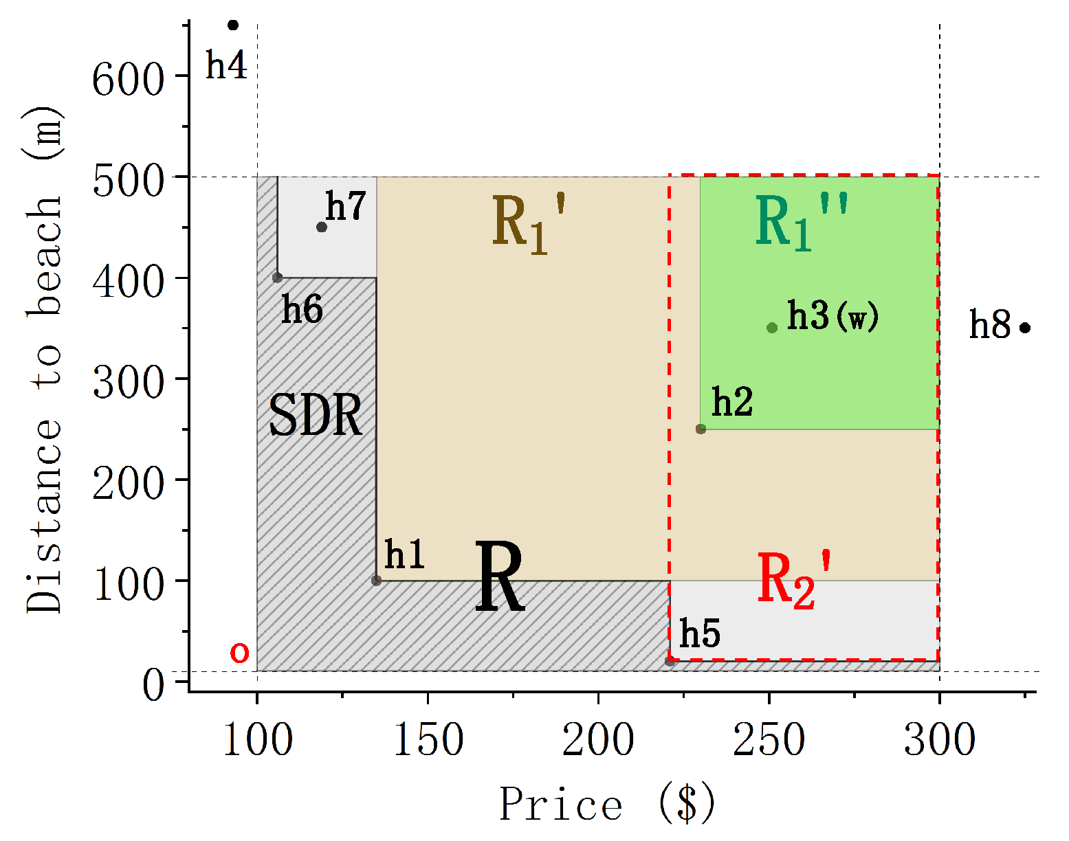
Suppose a newly-wed couple is going to Nassau for their honeymoon. They already have the expected hotel, but they still want to know which hotels (https://www.booking.com) are cheap near the beach. In Figure 1, we execute a skyline query on all Nassau hotels and get skyline points: $\{s{p}_1,s{p}_2,s{p}_3\}$. Although $s{p}_1$ and $s{p}_2$ are cheap, they are youth hostels but not romantic at all for lovers. Moreover $s{p}_3$ is too close to the beach. To solve this problem, they can set the values of attributes which can be accepted. Let the price range be 100 $–300 $ and the distance range from the beach be 10 m–500 m. The new skyline points based on the data in the orthogonal range R (i.e., the shaded area) can be found as $\{s{p}_1^{\prime },s{p}_2^{\prime },s{p}_3^{\prime }\}$. This means that they may be more interested in hotels $\{s{p}_1^{\prime },s{p}_2^{\prime },s{p}_3^{\prime }\}$. They only need to choose one of them, which greatly saves screening time. Consider the expected hotel is $h_2$ in Figure 2a. Why is $h_2$ not in the query results? This is the problem to be solved in this paper, that is, why-not questions in ORSQ.

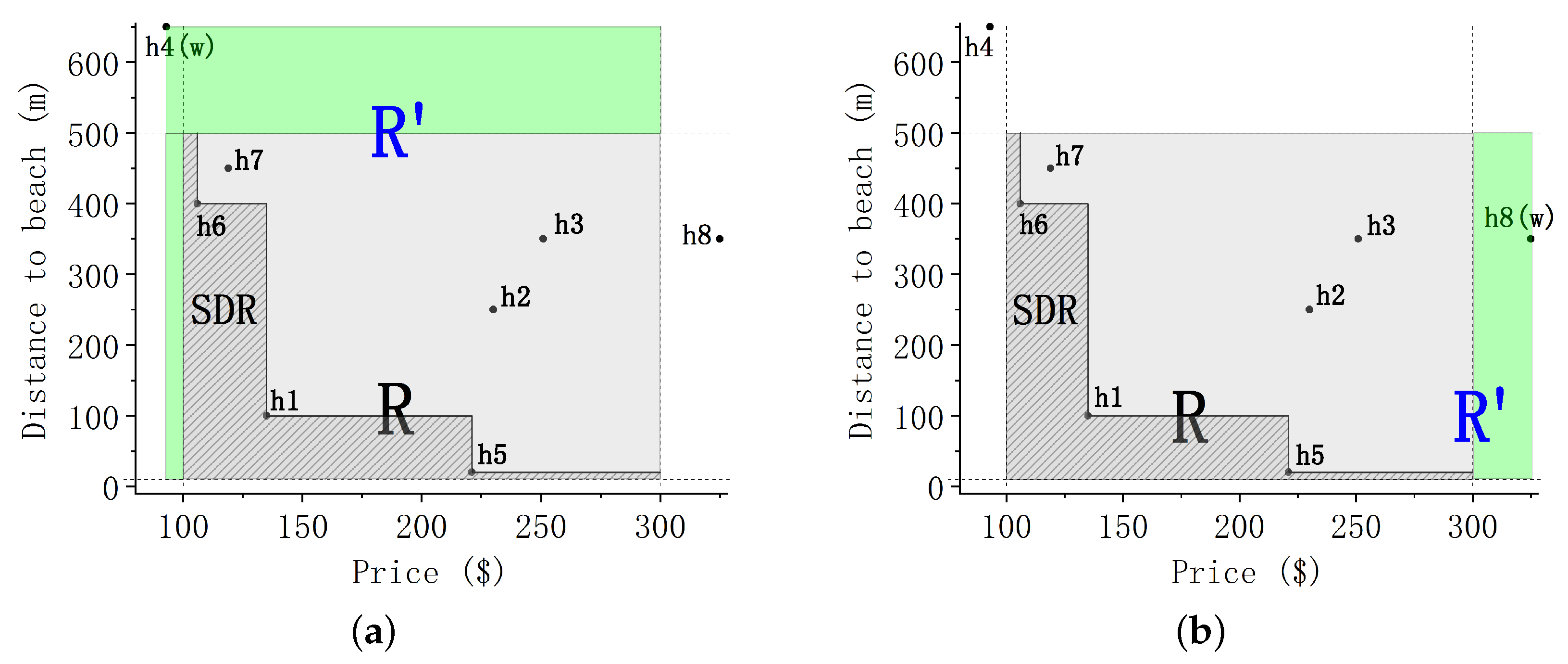
There are two main objectives of this paper. On the one hand, it is necessary to find out why the expected tuple does not appear in the result of ORSQ. On the other hand, we need to answer how to include the tuple in the result of ORSQ. Hereinafter, Figure 2 will be used as examples. For a more concise and clear explanation, we extract some data from Figure 1 as explanatory data (i.e., Figure 2b), and the corresponding ORSQ is shown in Figure 2a.

In summary, this paper aims to answer why-not questions in ORSQ. First of all, we answer why there is a “why-not” question. Secondly, we illustrate strategies of modifying the why-not point and the orthogonal range by analyzing the causes, so that the query results include the why-not point. For these strategies, we propose cost formulas. It is understood that this is the first attempt to research the why-not questions in skyline queries based on the orthogonal range. The main contributions of this paper are summarized as follows:

• Provide the meaning and semantics of the why-not questions in ORSQ.
• Propose strategies for modifying the why-not point and the orthogonal range according to the cause of the problem.
• Present how to modify the why-not point and the orthogonal range so that the why-not point is included in results.
• Prove algorithms with experiments.

This is the organizational structure of the paper. In the second section, we review the related work. In the third section, we describe the preliminary knowledge. According to the location of the why-not point, the fourth section describes how to solve the why-not questions in ORSQ by modifying the why-not point or the orthogonal range. In the fifth section, the experimental results are presented in terms of effectiveness and performance. In the sixth section, we summarize the paper.

2. Related Work

Range-based preference query. Wang et al. [13] first tried to solve the problem of dynamic skyline calculations considering range queries. To solve it, they proposed an effective algorithm based on the grid index and a novel variant of the well-known Z-order curve. Kalavagattu et al. [14] considered the problem of the dominating point set in two-dimension. Given an orthogonal query rectangle, the dominant point set is found in it. Rahul and Janardan [15] researched algorithms for range-skyline queries. Lin and Xu et al. [16] researched range-based skyline queries in mobile environments, and proposed two algorithms: index-based and not based on any index. Jiang et al. [17] and Fu et al. [18] researched continuous range-based skyline queries problem in road networks. Li et al. [19] researched why-not questions of Top-k queries on the orthogonal region. They adjusted the initial query by automatically updating the query so that the result of the new query contains why-not points with minimum cost.

Why-Not questions. Researchers have mainly proposed five explanations to answer why-not questions. First of all, operation positioning [20,21,22] refers to finding out the operation that causes the expected result to be lost. Secondly, data modification [23,24,25,26] refers to inserting new data or modifying existing data to make the missing tuple into query results. Thirdly, query refinement [27] refers to updating the query so that the new query results contain the missing tuple. Next, the key to the ontology-based approach [28] is to get a most-general explanation for why-not questions with the ontology provided by the user or automatically generated from data and patterns. Finally, the hybrid explanation [29,30] encompasses the variety of previously defined types of explanations to explain a larger set of missing-answers. Although operation positioning and ontology-based approach explain the reason for the expected tuple loss, they cannot help users solve the problem of expected tuple loss.

Why-Not questions in variant skyline queries. Islam and Zhou et al. [31] answered why-not questions in reverse skyline queries. They used data modification and query refinement strategies to propose solutions: (1) modify the data separately, (2) modify the query separately and (3) the integration of the above solutions. Miao et al. [32] made the greatest contribution to this paper. They researched “why-not” questions in range-based skyline queries in road networks. To deal with it, they proposed three strategies: (1) modifying the query range, (2) modifying the attributes of the why-not point and (3) modifying both of them. It is worth noting that their range refers to the range of distance. The orthogonal range in this paper is based on orthogonal regions proposed by Li et al. [19].

As far as we know, there is not much research to solve the why-not question in skyline queries. Next, we will formally define and formalize "why-not" questions in ORSQ, and then propose solutions based on data modification and query refinement technologies.

3. Preliminaries

Let $D=(D^1,\dots ,D^d)$ be a d-dimensional data space, $O\subseteq D$ is the dataset of objects, $E\subseteq O$ is the dataset of objects users expect and $R\subseteq O$ is the dataset of objects within the orthogonal query range. Each $D^i$ represents the i-th dimension and consists of numeric values only. Point $o\in O$ is expressed as $o=\{o^1,\dots ,o^d\}$, where $o^i\in D^i$ and $i\in \{1,\dots ,d\}$. Similarly, point $e\in E$ is expressed as $e=\{e^1,\dots ,e^d\}$. Dataset $R_i\subseteq D^i$ represents the range of the i-th dimension, where $R\subseteq R_i$. Firstly, we relate the definitions of orthogonal range, skyline query (i.e., SQ), skyline query based on orthogonal range (i.e., ORSQ) and skyline dominance region (i.e., SDR). We then introduce the definition of why-not questions in ORSQ.

Definition 1

(Orthogonal range). Given a dataset of objects O, ranges of attributes $R_i$ and $R_i\subseteq O$, the orthogonal range specifies the users’ retrieval range R, where $R=R_1\cap \dots \cap R_d$ iff $\forall i\in \{1,\dots ,d\}$, $v_1^i\in D^i$, $v_2^i\in D^i$ : $v_1^i\le R_i\le v_2^i$.

Equivalently, the orthogonal range refers to the intersection of ranges in each dimension which are continuous and non-segmented. Take Figure 2a for example. Let $d=2$, the attributes are the hotel price and the distance from the hotel to the beach. The range of price is $R_1(100\$\le R_1\le 300\$)$, and the range of distance from hotel to beach is $R_2(100$ m $\le R_2\le 5000$ m). The shaded part is the orthogonal range R, where $R=R_1\cap R_2$ and the points in R are $\{h_1,h_2,h_3,h_5,h_6,h_7\}$. When executing a query, we only need to search in R. This is very effective in improving query efficiency and can provide users with query results that better meet their needs.

Definition 2

(Skyline Query). Given a dataset of objects O, the skyline query SQ retrieves all points $o\in O$ that are not dominated by any other points. These points are also called Skyline Points (i.e., SP), where SP $\subseteq O$. Point $o_1$ dominates point $o_2$ iff (1) $\forall i\in \{1,\dots ,d\}$ : $o_1^i\le o_2^i$ and (2) $\exists j\in \{1,\dots ,d\}$ : $o_1^j<o_2^j$.

In a nutshell, skyline queries focus on the definition of dominance. Take Figure 1 for example, where we execute a skyline query on all hotels and get SP $=\{s{p}_1,s{p}_2,s{p}_3\}$. Point $s{p}_2^{\prime }\notin$ SP because $s{p}_2$ and $s{p}_3$ dominate $s{p}_2^{\prime }$.

Lemma 1.

Let $s{p}_i\in$ SP, $i\in \{1,\cdots ,n\}$. If $n\ge 2$, SP are distributed in a stepwise manner.

Proof. 

Prove it in a two-dimensional space Firstly. Assume that in $D^1$, they are arranged in the order of $s{p}_1^1\le s{p}_2^1\le \cdots \le s{p}_n^1$. Suppose they have coincident points, namely, $\exists i,j\in \{1,\cdots ,n\}$ and $i\ne j$ : $s{p}_i^1=s{p}_j^1$. Then, unless $s{p}_i^2=s{p}_j^2$, there will always be points that are dominated. However, this is inconsistent with the given condition that they are all skyline points. Next, let us assume that in $D^1$ $\forall i,j\in \{1,\cdots ,n\}$ and $i<j$ : $s{p}_i^1<s{p}_j^1$. Since they are not dominated by any points, there must be $s{p}_i^2>s{p}_j^2$. That is, $s{p}_1,s{p}_2,\cdots ,s{p}_n$ are arranged in a ladder. In high dimensional space, the same can be proved. □

Definition 3

(Skyline query based on orthogonal range). Given a dataset of objects O and the orthogonal range $R\subseteq O$. In ORSQ, users execute SQ in R to find skyline points (i.e., SP$\left(R\right)$) that they might be interested in.

In Figure 1, the skyline query without a limited query range gets SP $=\{s{p}_1,s{p}_2,s{p}_3\}$. These hotels have their shortcomings and do not meet the needs of all users. The traditional skyline query blindly chooses the best result in the whole range, but it is not always helpful to users. Therefore, in Figure 2a, we specify the orthogonal query range R, and get SP$\left(R\right)=\{h_1,h_5,h_6\}$. This helps users find information they are more interested in by considering their actual consumption level and preferences.

Definition 4

(Skyline Dominance Region). Points in SDR are not dominated by any skyline points.

Take Figure 2a for instance. The slant shaded region is the dominant region of the skyline query based on R. Points in SDR cannot be dominated by any points in the query range. It is worth noting that the boundary of SDR is related to skyline points.

Lemma 2.

SDR boundary is determined by the query range and straight lines passing through skyline points coordinate and parallel to the coordinate axis.

Proof. 

Let SP $=\{s{p}_1,\dots ,s{p}_n\}$ and $i\in \{1,\dots ,n\}$. Each line is equivalent to treating skyline points as the origin respectively and dividing the coordinate axis again. According to Definition 2, we can easily get that points $o\in O$ in the upper right corner of the coordinate chart are always dominated by certain skyline points. Equivalently, $\exists o\in O$ and $\exists j\in \{1,2,\dots ,d\}$ : $s{p}_i^j<o^j$. Therefore, we have to exclude the upper right corner of each skyline point. In addition, the boundary of SDR also needs to consider the boundary of the query range. □

Definition 5

(Why-not questions in ORSQ). Given a dataset of objects O, the orthogonal range $R\subseteq O$ and the expected object $e\in O$. There are three different aspects of why-not questions in ORSQ: (1) find out why e does not appear in SP$\left(R\right)$; (2) propose solutions so that the why-not point w is included in the query result of ORSQ; (3) find the optimal solution and minimize the cost of solving the problem.

For the first aspect, according to Definition 3, $e\notin$ SP$\left(R\right)$ has two reasons: (1) e is in the orthogonal query range, but it is dominated by other points in the range; (2) e is not within the orthogonal query range. Take Figure 2a as an example, points in the orthogonal range R are $\{h_1,h_2,h_3,h_5,h_6,h_7\}$ and SP$\left(R\right)=\{h_1,h_5,h_6\}$. If $e=h_2$, then $e=w$. Because $h_2$ is dominated by $h_1$. If $e=h_4$, then $e=w$. Because $h_4\notin R$.

For the second and third problems, we have to propose different solutions for different reasons. When (1) $w\in R$, we have three solutions: (1) modify the why-not point w, (2) narrow the orthogonal range R and (3) the integration of the above solutions. When (2) $w\notin R$, it is necessary to expand R to $R^{\prime }$ so that $w\in R^{\prime }$. We then test whether e is included in SP$\left(R^{\prime }\right)$. If $e\in$ SP$\left(R^{\prime }\right)$ then the problem is resolved, otherwise the problem is returned to (1). The following is a brief explanation of the application and implementation steps of these solutions.

Modify w. The main idea is to modify w to $w^{\prime }$ so that $w^{\prime }\in$ SP$\left(R\right)$. It involves Definition 4. This solution preserves the initial skyline points and provides users with information similar to w.

Modify R. The main idea is to modify R to $R^{\prime }$ so that $w\in$ SP$\left(R^{\prime }\right)$. It includes two strategies: expanding R and narrowing R. When $w\notin R$, we expand R. When $w\in R$, there must be $s{p}_i$ dominates w, where $s{p}_i\in$ SP$\left(R\right)$ and $i\in \{1,\dots ,n\}$. The fact cannot be changed even if R is expanded. So we narrow R and exclude the skyline points that dominate w. Last but not least, narrowing the range will lose the original skyline points, although it is also possible to get new skyline points different from w. In this solution, extracting orthogonal range data is the key. The calculation steps are as follows: (1) Input file name of original data $originalData$, file name of extracted data $generateData$, the orthogonal range R and the flag $fg$. Parameter $fg=True$ when extracting orthogonal range data during an initial query or expanding the orthogonal range; $fg=False$ when narrowing the orthogonal range. (2) Initialize the extraction result $result$ to $False$. Read the maximum and minimum values in each dimension from R. And then judge whether values are reasonable. If reasonable, $result=True$, otherwise return $result$. (3) Then open and read $originalData$, open and write $generateData$. (4) Traversing the data in $originalData$, and writing the data into $generateData$ if there is data matching the orthogonal range. (5) Close $originalData$, $generateData$ and return $result$.

Modify both of them. The above solutions have their advantages and disadvantages. If the difference between w and $w^{\prime }$ is large or the narrowed range is too small, this has no practical significance. To this end, we can combine these solutions to provide a compromise solution.

In this paper, we focus on the second and third aspects. The first problem is easy to calculate. Focusing on the second aspect, we can propose solutions based on the distribution of w. The steps to solve why-not questions in ORSQ are as follows. Firstly, we judge whether w is included in R. If $w\in R$, we select a solution among modifying the why-not point (i.e., MWP), narrowing the orthogonal range (i.e., MRN) and the integration of the above solutions (i.e., MWR). If not, we expand the orthogonal range (i.e., MRE). If the problem still exists, we choose one of the above three solutions. However, an algorithm may produce a variety of answers, such as the MWR algorithm. Considering the third question, we can find the answer with the minimum cost. The pseudo-code of the total algorithm of the why-not questions in ORSQ is shown in Algorithm 1.

Algorithm 1 Why-Not questions in ORSQ

1: $flag1\leftarrow isInRange\left(\right)$ 2: if$flag1$then 3:  $//$If the why-not point is in the range, we select a strategy from MWP, MRN and MRW. 4: else 5:   MRE()  $//$Modify and Expand the Orthogonal Range 6:   $flag2\leftarrow$ ORSQ() 7:   $//$Execute a skyline query in the new range to judge whether the why-not question is solved. 8:   if $flag2$ then 9:    $//$If the problem is not solved, we select a strategy from MWP, MRN and MRW. 10:   end if 11: end if

4. Solutions to Why-Not Questions in ORSQ

In this section, we will present how to modify the why-not point w and the orthogonal range R according to whether w is within R, and include the why-not point in the new query results with minimum cost. We discuss solutions in three cases: (1) $d=2$ and $w\in R$; (2) $d=2$ and $w\notin R$; (3) $d>2$ and $w\notin R$. For more specific explanations, we use hotels as objects in the examples.

4.1. Case 1: $d=2$ and $w\in R$

When $w\in R$ but $w\notin$ SP$\left(R\right)$, we have three algorithms to make the new query results contain the why-not point, namely modifying the why-not point (i.e., MWP algorithm), narrowing the orthogonal range (i.e., MRN algorithm), and the integration of the above algorithms (i.e., MWR algorithm).

4.1.1. Modifying the Why-Not Point

Definition 6

(MWP). Given a dataset of hotels H, the orthogonal range $R\subseteq H$ and the expected hotel $e\in R$. When $e\notin$ SP$\left(R\right)$(i.e., $e=w$), modify the why-not point w to $w^{\prime }$, so that $w^{\prime }\in$ SP$\left(R\right)$. And the cost in Formula (1) should be as small as possible.

$$cost(w,w^{\prime })=|w-w^{\prime }|=\frac{|dist(w,o)-dist(w^{\prime },o)|}{dist(w,o)}$$

(1)

Assuming that $h_i,h_j\in H$ where $i,j\in \{1,2,\cdots ,n\}$ and $i\ne j$. Let $d=2$, $h\in H$ is expressed as $h=\{h^1,h^2\}$. The Euclidean distance between them is calculated as Formula (2).

$$|h_i{h}_j|=\sqrt{{(h_i^1-h_j^1)}^2+{(h_i^2-h_j^2)}^2}$$

(2)

In Formula (1), point $o\in R$ is a point whose coordinates correspond to the minimum values of R in each dimension, and $dist(w,o)$ represents the Euclidean distance between w and o. Similarly, $dist(w^{\prime },o)$ represents the Euclidean distance between $w^{\prime }$ and o. The cost of the MWP algorithm reflects the difference before and after the modification of w.

As shown in Figure 3, point $e=h_3$ is the why-not point w because points $\{h_1,h_5\}$ dominates $h_3$. To modify w to $w^{\prime }\in$ SP$\left(R\right)$, we need to find the moving region. In this moving region, the why-not point can dominate all points within R and cannot be dominated by any other points. However, considering the practical significance, when w is modified to $w^{\prime }\in$ SDR, users can only get SP$\left(R\right)=\left\{w^{\prime }\right\}$. Therefore, we need to find a critical condition that will not lose the original skyline points and will also provide points that users may be interested in. That is, we need to find points in the boundary of SDR that has the shortest Euclidean distance from w to $w^{\prime }$. These points are generated in a candidate set C, which includes mapping points $C_{mp}$ from w to skyline points and turning points $C_{tp}$ between skyline points, where $C=C_{mp}\cup C_{tp}$. In Figure 3, $e=w$ and $C_{mp}=\{B,D\}$, $C_{tp}=\{A,C\}$. Obviously, in $\Delta wB{h}_1$, $dist(w,B)<dist(w,h_1)$ because $\angle B{h}_{1}w<\angle wB{h}_1$. Similarly, we get these facts that $dist(w,C)<dist(w,h_1)$, $dist(w,A)<dist(w,h_6)$ and $dist(w,D)<dist(w,h_5)$. We can get the fact: $\forall i\in \{1,\dots ,n\}$ and $\forall j\in \{1,\dots ,k\}$, $dist(w,b{p}_i)\ge dist(w,c_j)$ where $c_j\in C$, $b{p}_i\in BP$ and $BP$ is a point set on the SDR boundary.

In a few words, the MWP algorithm is to find a candidate set. We calculate turning points $C_{tp}$ between skyline points firstly. Let $d=2$, the number of points in SP$\left(R\right)$ is n and SP$\left(R\right)$ arranged in ascending order according to $D^1$. The point of $C_{tp}$ consists of the abscissa of the next skyline point and the ordinate of the current skyline point. As shown in Formula (3).

$$C_{tp}=\left\{(s{p}_{i+1}^1,s{p}_i^2)\right\};s{p}_i\in SP\left(R\right),i\in \{1,\cdots ,n-1\},s{p}_i^1<s{p}_{i+1}^1$$

(3)

Next, we calculate $C_{mp}$. The coordinates of $C_{mp}$ are related to the arrangement order of SP$\left(R\right)$ and w on each coordinate. Firstly, we merge SP$\left(R\right)$ and w into a list $skylineW$, and then sort the list by $D^1$ and $D^2$ respectively to obtain $ox$ and $oy$. Later, we find out the order $wpxo$ of the abscissa of w in $ox$, $wpyo$ of the ordinate of w in $oy$. The general formula of $C_{mp}$ is given below:

$$C_{mp}=\{(o{x}_{wpxo}^1,o{x}_{wpxo-1}^2),(o{y}_{wpyo-1}^1,o{y}_{wpyo}^2)\}$$

(4)

Finally, we find the point with the shortest Euclidean distance from w in C. We define the cost of the MWP algorithm in Formula (1). The closer the point is to point o, the smaller the cost is. But compared to the cost, users prefer the change of w as small as possible. Algorithm 2 gives the pseudo-code for all of the above calculation steps.

Algorithm 2 MWP(w, SP$\left(R\right)$)

Input:w: the coordinates of the why-not point; SP$\left(R\right)$: Results obtained after executing SQ$\left(R\right)$ Output:$w^{\prime }$: the modified why-not point 1: $orderSPX\leftarrow$ sorted(SP$\left(R\right)$, $s{p}^1$), 2: $length\leftarrow len\left(orderSPX\right)$ 3: $//$Calculate $C_{tp}$ 4: for i in range(length) do 5:  if i + 1 < length then 6:   $d\leftarrow distance(w,(s{p}_{i+1}^1,s{p}_i^2))$ 7:   $C.append\left([s{p}_{i+1}^1,s{p}_i^2,d]\right)$ 8:  end if 9: end for 10: $//$Calculate $C_{mp}$ 11: $skylineW\leftarrow$ SP$\left(R\right)$ 12: $wpx,wpy\leftarrow w$ 13: $skylineW.append\left(\right[wpx,wpy\left]\right)$ 14: $ox\leftarrow sorted(skylineW,o{x}^1)$ 15: $oy\leftarrow sorted(skylineW,o{y}^2)$ 16: $wpxo\leftarrow search(ox,wpx)$ 17: $wpyo\leftarrow search(oy,wpy)$ 18: $d\leftarrow distance(w,(o{x}_{wpxo}^1,o{x}_{wpxo-1}^2))$ 19: $//$$C_{mp}$ for X 20: $C.append\left([o{x}_{wpxo}^1,o{x}_{wpxo-1}^2,d]\right)$ 21: $d\leftarrow distance(w,(o{y}_{wpyo-1}^1,o{y}_{wpyo}^2))$ 22: $//$$C_{mp}$ for Y 23: $C.append\left([o{y}_{wpyo-1}^1,o{y}_{wpyo}^2,d]\right)$ 24: $orderDistance\leftarrow sorted(C,C^3)$ 25: $w^{\prime }\leftarrow orderDistance\left[0\right]$  $//w^{\prime }$ 26: return$w^{\prime }$

Example: Consider the shaded part given in Figure 3 is the orthogonal range R, the expected point $e=h_3$ is the why-not point w and results of SQ$\left(R\right)$ are SP$\left(R\right)=\{h_1,h_5,h_6\}$. According to Algorithm 2, $C_{tp}$ = {[A(135,400),126.31], [C(221,100),251.79]}, $C_{mp}$ = {[B(135,350),116.00], [D(251,20),330.00]}. And $orderDistance$ = {(B,116.00), (A,126.31), (C,251.79), (D,330.00)}. This means that users can replace w with point B(135,350) and take it into account.

Complexity analysis: The complexity of MWP is mainly determined by calculating the candidate set C and sorting C by Euclidean distance. In addition, the calculation of the Euclidean distance in steps 6, 18, 21 can be considered to be completed in constant time. Moreover, the complexity of calculating $C_{tp}$ in steps 4–9 is $O\left(N\right)$, and the complexity of calculating $C_{mp}$ in steps 11–23 is mainly the complexity of Python’s built-in list sorting (i.e., $O(N\ast lo{g}_{2}N)$) and binary search ($O\left(lo{g}_{2}N\right)$). Similarly, the complexity of sorting C in step 24 is also ($O(N\ast lo{g}_{2}N)$). Therefore, the overall complexity of MWP is $O(N\ast lo{g}_{2}N)$.

4.1.2. Narrowing the Orthogonal Range

Definition 7

(MRN). Given a dataset of hotels H, the orthogonal range $R\subseteq H$ and the expected hotel $e\in R$. When $e\notin$ SP$\left(R\right)$(i.e., $e=w$), narrow R to $R^{\prime }$, so that the why-not point $w\in$ SP$\left(R^{\prime }\right)$. Moreover, the cost in Formula (5) should be as small as possible.

$$cost(R,R^{\prime })=|R-R^{\prime }|=\frac{|S\left(R\right)-S\left(R^{\prime }\right)|}{S\left(R\right)}$$

(5)

Parameter S represents the space of R. If $d=2$, R is a rectangle and $S\left(R\right)$ represents the area of R. If $d=3$, R is a cuboid and $S\left(R\right)$ represents the volume of R. Other dimensions are analogous. The cost of MRN reflects the difference between R and $R^{\prime }$.

In Figure 4, point $e=h_3$ and e is the why-not point. To narrow R to $R^{\prime }$ and $w\in$ SP$\left(R^{\prime }\right)$, we must exclude some skyline points SP${\left(R\right)}_{part}=\{h_1,h_5\}$ that dominate w. The steps for calculating SP${\left(R\right)}_{part}\subseteq$ SP$\left(R\right)$ are as follows: (1) Merge w and SP$\left(R\right)$ into a list $skylineW$, arrange it as $ox$ from small to large in $D^1$. (2) Find the position $wpxo$ of w in $ox$. (3) Set $wpxo$ as the loop length and traverse $ox$. If $o{x}_i^2\le w_i^2$ where $i\in \{1,2,\dots ,wpxo\}$, this indicates that the current skyline point $o{x}_i$ dominates w.

The narrowed range is determined by the coordinates of SP$\left(R\right)$ and the boundary of R. The boundary of the narrowed range is calculated as follows: (1) Calculate SP${\left(R\right)}_{part}$ that dominate w. Point $s{p}_i\in$ SP${\left(R\right)}_{part}$ is expressed as $s{p}_i=\{s{p}^1,s{p}^2,\cdots ,s{p}^d\}$, $i\in \{1,2,\cdots ,k\}$. (2) Calculate $R^{\prime }$ as shown in Formula (6), the narrowed range $R^{\prime }$ is determined by the coordinates of SP${\left(R\right)}_{part}$ and the boundary of R. (3) After narrowing R for the first time, we execute SQ($R^{\prime }$) to judge whether the why-not question exists. If it still exists, repeat the above steps until the problem is solved. (4)Next, the corresponding narrowed range is calculated at the next point in SP${\left(R\right)}_{part}$. (5)Finally, we will get some narrowed ranges. The final result is the result with minimum cost. Algorithm 3 gives the pseudo-code for all of the above calculation steps.

$$\begin{array}{c}\hfill SP{\left(R\right)}_{part}=\left\{(s{p}_i^1,s{p}_i^2)\right\},i\in \{1,2,\cdots ,k\}\\ \hfill R^{\prime }=\left\{(s{p}_i^1\le D^1\le xmax,s{p}_i^2\le D^2\le ymax)\right\},SP{\left(R\right)}_{part}\notin R^{\prime }\end{array}$$

(6)

Example: Take Figure 4 for example. The shaded area is the original orthogonal range R. Let the expected point $e=h_3$, and get SP$\left(R\right)=\{h_1,h_5,h_6\}$. According to the method of calculating SP${\left(R\right)}_{part}$, SP${\left(R\right)}_{part}=\{h_1,h_5\}$ ($k=2$). For $h_1$, R is first narrowed to $R_1^{\prime }$ and SP${\left(R_1^{\prime }\right)}_{part}=\left\{h_2\right\}$. However, the why-not point w is dominated by $h_2$ and the problem still exists. Based on $R_1^{\prime }$, we further narrow down the range to $R_1^{″}$ and SP${\left(R_1^{″}\right)}_{part}=\varnothing$, the problem is solved. Similarly, for $h_5$, R is first narrowed to $R_2^{\prime }$ and SP${\left(R_2^{\prime }\right)}_{part}=\left\{h_2\right\}$. Then, we further narrow down the range to $R_2^{″}$ based on $R_2^{\prime }$, which $R_2^{″}=R_1^{″}$. Finally, we can get the narrowed range $R_1^{″}$.

Complexity analysis: The complexity of MRN is mainly consists of sorting $skylineW$ in step 6 (i.e., $O(N\ast lo{g}_{2}N)$), finding the position of the abscissa of w in $ox$ in step 7 (i.e., $O\left(lo{g}_{2}N\right)$) and traversing SP${\left(R\right)}_{part}$ in steps 8–22. Suppose there are n elements in SP(R) and k elements in SP${\left(R\right)}_{part}$. The best case is that each point in SP${\left(R\right)}_{part}$ only needs to be narrowed by once, and the complexity is $O(k\ast |SQ\left(R\right)\left|\right)$, where SQ(R) represents the complexity of ORSQ and is equal to $O(N\ast logN)$. On the other hand, the worst case is that we need to narrow the range multiple times until no skyline points dominate w. Suppose that the problem is solved after M cycles ($M>k$). Then, the complexity is $O(M\ast |$SQ$\left(R\right)\left|\right)$. Consequently, the overall time complexity of MRN is $O(M\ast N\ast logN)$.

Algorithm 3 MRN (w, SP$\left(R\right)$, R)

Input:w: the coordinates of the why-not point; SP$\left(R\right)$: Results of SQ$\left(R\right)$; R: the original orthogonal range Output:$R^{\prime }$: the narrowed orthogonal range 1: $wpx,wpy\leftarrow w$ 2: $skylineW\leftarrow$ SP$\left(R\right)$ 3: $xmin,xmax,ymin,ymax\leftarrow R$ 4: $S\leftarrow |xmax-xmin|\ast |ymax-ymin|$ 5: $skylineW.append\left(\right[wpx,wpy\left]\right)$ 6: $ox\leftarrow sorted(skylineW,s{w}^1)$ 7: $wpxo\leftarrow search(ox,wpx)$ 8: for i in range($wpxo$) do 9:  if $o{x}^2\le wpy$ then 10:   $nxmi\leftarrow o{x}^1,nymi\leftarrow o{x}^2$ 11:   $R^{\prime }\leftarrow nxmi,xmax,nymi,ymax$ 12:   SP$\left(R^{\prime }\right),flag\leftarrow SQ(R^{\prime },w)$ 13:   if not $flag$ then 14:    $//$If $flag$ is $False$, the why-not question still exists. 15:    MRN$(w,SP\left(R^{\prime }\right),R^{\prime })$ 16:   else 17:    $S^{\prime }\leftarrow |xmax-nxmi|\ast |ymax-nymi|$ 18:    $cost\leftarrow |S-S^{\prime }|/S$ 19:    $//$Save $R^{\prime }$ and $cost$ 20:   end if 21:  end if 22: end for 23: return$R^{\prime }$

4.1.3. Modifying the Why-Not Point and Narrowing the Orthogonal Range

As we have already analyzed, we will not lose the initial skyline points if we apply the MWP algorithm. If the difference between w and $w^{\prime }$ is too large, it is meaningless. Moreover, if we narrow the range R, we will lose the existing skyline points, although we may get new skyline points. If the narrowed range is too small, we also have no choice, and this is not what we want to see. To solve the above two problems, a hybrid method of modifying w and narrowing R is proposed. This approach can neutralize two problems to expect a compromise result. We hope to narrow R to $R^{\prime }$ to get points that we might be interested in that are closer to w. If necessary, we modify w. We formally define the MWR algorithm as follows:

Definition 8

(MWR). Given a dataset of hotels H, the orthogonal range $R\subseteq H$ and the expected hotel $e\in R$. When $e\notin$ SP$\left(R\right)$(i.e., $e=w$), narrow R to $R^{\prime }$, and if necessary, modify the why-not point w to $w^{\prime }$, so that $w^{\prime }\in$ SP($R^{\prime }$). And the cost in Formula (7) should be as small as possible.

$$cost(w^{\prime },R^{\prime })={\lambda }_1\ast cost(w,w^{\prime })+{\lambda }_2\ast cost(R,R^{\prime })$$

(7)

As shown in Formula (7), we will discuss the cost of MWR according to the situation. When only w is modified, ${\lambda }_1=1$ and ${\lambda }_2=0$. When only R is modified, ${\lambda }_1=0$ and ${\lambda }_2=1$. When both are modified, ${\lambda }_1=0.5$ and ${\lambda }_2=0.5$.

When there is only one type of result: (1) Only w is modified, the final result is the scheme with the smallest Euclidean distance. (2) Only R is modified, the final result is the scheme with the minimum cost. (3) Both w and R are modified, results of the shortest Euclidean distance in the same range are first selected, and the one with the minimum cost of these results is the final result. When the result contains multiple types of results, that is, it includes condition(a): only narrowing R, and condition(b): narrowing R and modifying w. We obtained two final solutions according to (2) and (3), respectively.

To avoid meaningless narrowing, we need to determine the limit of the narrowed range. Here, we stipulate that only one skyline point dominates w is the limit. The main steps of the MWR algorithm are as follows: (1) Calculate $count$, which is the number of points in SP${\left(R\right)}_{part}$. (2) If $count=1$, we execute the MWP algorithm. (3) If $count\ne 1$, after narrowing the orthogonal range once, we execute SQ$\left(R^{\prime }\right)$ to determine whether the problem exists. (4) If the problem persists, return to (1). (5) If not, return parameters of the current range.

Example: Take Figure 5 for illustration. The shaded area is the original orthogonal range R. In Figure 5a, let the expected point $e=h_7$, and get SP$\left(R\right)=\{h_1,h_5,h_6\}$. Point $e=h_7$ is the why-not point w, because $h_6\in$ SP$\left(R\right)$ dominates w. Through the MWR algorithm, we first calculate the number of points in SP${\left(R\right)}_{part}$ and $count=1$. In this case, directly modify w. In Figure 5b, let $e=h_3$. Because points $\{h_1,h_5\}$ dominate e, $count=2$. We first narrow down the range to $R^{\prime }$ to get SP$\left(R^{\prime }\right)=\left\{h_2\right\}$. Then, recalculate $count=1$. At this time, directly modify w in $R^{\prime }$.

Complexity analysis: The complexity of MWR consists mainly of (1) calculating the number of elements of SP${\left(R\right)}_{part}$, (2) MWP (i.e., $O(N\ast lo{g}_{2}N)$) and (3) narrowing the orthogonal range until it reaches the limit. According to the calculation steps mentioned above, the complexity of (1) is $O(N\ast lo{g}_{2}N)$. The complexity of (3) is similar to the complexity of MRN, except when $flag$ is $False$, MWR is re-executed instead of MRN. Combined with the complexity of MRN, the complexity of (3) is $O(M\ast N\ast logN)$. Therefore, the overall complexity of the MWR algorithm is $O(M\ast N\ast logN)$.

4.2. Case 2: $d=2$ and $w\notin R$

In Section 4.1, we discussed how to solve why-not questions in ORSQ when w is in R. Next, we will discuss another case: w is not in R. Considering that the distribution of w is random, the two-dimensional space is divided as shown in Figure 6, where R is the orthogonal query range (shaded region). When $w\notin R$, then it may be distributed in A1–A4, B1–B2, or C1–C2.

Obviously, when $e\notin R$, $e\notin SP\left(R\right)$. This means that e is the why-not point w. Moreover, the new query results cannot contain w simply by modifying the why-not point and narrowing the orthogonal range. Because SQ$\left(R\right)$ retrieves data in R. Therefore, we need to expand the orthogonal range so that w is included in the new orthogonal range. We formally define the MRE algorithm as follows.

Definition 9

(MRE). Given a dataset of hotels H, the orthogonal range $R\subseteq H$ and the expected hotel $e\notin R$. When $e\notin$ SP$\left(R\right)$(i.e., $e=w$), expand R to $R^{\prime }$ so that $w\in R^{\prime }$. The problem is then converted to Case 1. Moreover, the cost in Formula (8) should be as small as possible.

The cost of the MRE algorithm is discussed separately. When $w\in$ SP$\left(R^{\prime }\right)$, the cost is the same as Formula (5). When $w\notin$ SP$\left(R^{\prime }\right)$, the cost depends on the solution chosen.

The calculation steps of the MRE algorithm are as follows: (1) Expand R to $R^{\prime }$. Obviously, the boundary of $R^{\prime }$ are related to the boundary of R ($xmin$, $xmax$, $ymin$, $ymax$) and the coordinates of w ($wpx$, $wpy$). The minimum value on the x-axis of $R^{\prime }$ is the smaller one between $wpx$ and $xmin$. The maximum value on the x-axis of $R^{\prime }$ is the larger one between $wpx$ and $xmax$. Other dimensions and so on. (2) Execute SQ$\left(R^{\prime }\right)$ to determine if the why-not question exist. (3) If it does not exist, the problem is solved. If it still exists, the problem is turned to Case 1 ($w\in R^{\prime }$).

$$\left\{\begin{array}{cc}cost(R,R^{\prime }),\hfill & w\in SP\left(R^{\prime }\right)\hfill \\ cost(w^{\prime },R^{\prime }),\hfill & w\notin SP\left(R^{\prime }\right),MWP\hfill \\ cost(R,R^{″}),\hfill & w\notin SP\left(R^{\prime }\right),MRN\hfill \\ cost(w^{\prime },R^{″}),\hfill & w\notin SP\left(R^{\prime }\right),MWR\hfill \end{array}\right.$$

(8)

Example: In Figure 7, the orthogonal range $R=\{h_1,h_2,h_3,h_5,h_6,h_7\}$, SP$\left(R\right)=\{h_1,h_5,h_6\}$. In Figure 7a, let point $e=h_4$ and e is the why-not point w. According to the MRE algorithm, we expand R to $R^{\prime }$ so that $w\in R^{\prime }$. Next, we calculate SP$\left(R^{\prime }\right)$ and get the conclusion that $w\in$ SP$\left(R^{\prime }\right)$. The why-not question has been solved. In Figure 7b, let point $e=h_8$, then $e=w$. Repeat the above steps and we find that $w\notin$ SP$\left(R^{\prime }\right)$. It is no longer possible to solve the problem by expanding the orthogonal range. The problem is changed to Case 1: the why-not point is in the query range.

Complexity analysis: The complexity of MRE is primarily related to expanding the orthogonal range (i.e., $O\left(1\right)$), skyline queries within the new range (i.e., $O\left(\right|$SQ(R)$\left|\right)$), and the strategy we choose in Case 1.

4.3. Case 3: $d>2$ and $w\notin R$

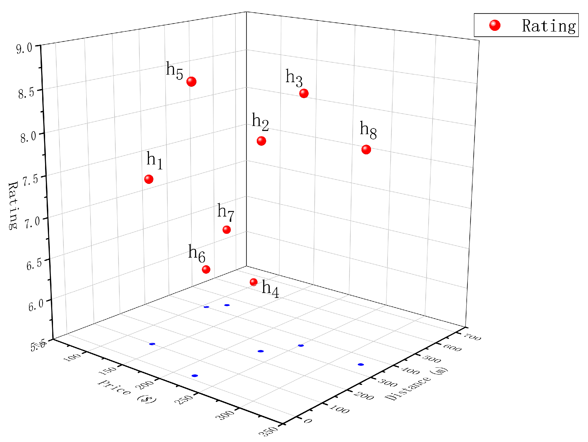
In the multidimensional case, the solution is similar to that in the two-dimensional case. If $w\notin R$, we need to expand R so that w is included in the new orthogonal range. Without a doubt, the change in R should be as small as possible. Take Figure 8 as an example. The attributes are the hotel price, the distance from the hotel to the beach and the hotel rating. The range of price is $R_1(100\$\le R_1\le 300\$)$, the range of distance is $R_2(100\mathrm{m}\le R_2\le 500\mathrm{m})$ and the range of rating is $R_3(7\le R_3\le 10)$. The orthogonal range $R=R_1\cap R_2\cap R_3$ and the points in R are $\{h_1,h_2,h_3,h_5\}$. If the expected hotel is $h_8$, we only need to expand $R_1$ to $100\$\le R_1^{\prime }\le 350\$$.

If the why-not point w is in the orthogonal range, we have three solutions:

Modify the why-not point. Firstly, we execute the skyline query in the new orthogonal range to find the boundary of the SDR region. Then, based on the boundary of the SDR, we find the range in which the why-not point can move, so that the modified why-not point is not dominated by any point, and the cost is as small as possible.

Narrow the orthogonal range. In order that the why-not point is not dominated by other points, we can narrow the orthogonal range so that the new orthogonal range contains the why-not point and does not contain the point that dominates w. When the result of the skyline query in the new orthogonal query range contains the why-not point, we stop narrowing the orthogonal range.

Narrow the orthogonal range and modify the why-not point if necessary. If the modified why-not point or the narrowed orthogonal range is too far from the expected effect, it has no good reference value and little significance to solve the problem. To this end, we can amend both at the same time in the hope of reaching a compromise solution.

5. Experimental Results and Discussion

We use Nassau’s real hotel dataset, namely a data set collected from Booking.com, and two types of synthetic data, namely anti-correlation data and independent data, of three different sizes (10 K, 50 K and 100 K tuples) to evaluate strategies for why-not questions in ORSQ. According to the method proposed by Borzsony et al. [33], we generate synthetic data sets. The real hotel dataset has properties related to price, distance to the beach, rating, etc. In the experiments, we considered in a two-dimensional space, two numerical properties, namely price, and distance to the beach. It is important to answer the “why-not” questions in real datasets. Take hotels as an example, travelers can find hotels more quickly according to their consumption levels and preferences and can get hotels closer to the why-not point, which is more in line with their expectations.

All experiments were performed on a 3.9 GHz central processor and 8.0 GB of main memory. We use the BBS algorithm to calculate skyline points. The page_size of BTree on the disk is 2048 bytes, the pointer_size is 4, and the key_size is 8. All algorithms proposed in this paper are implemented by Python. The experimental results will be shown below from the effectiveness and performance of the algorithms.

5.1. Effectiveness

In this section, we use Nassau’s hotel dataset to demonstrate the effectiveness of the algorithms. More specifically, the four different strategies proposed in this paper are: (1) only modify the why-not point (MWP). (2) only narrow the orthogonal range (MRN), (3) simultaneously modify the why-not point and narrow the orthogonal range (MWR), (4) expand the orthogonal range (MRE) and combine other strategies.

Firstly, we execute the skyline query on the dataset $H=[0,750]\ast [0,2900]$ with a price range of 0 $–750 $ and a distance range of 0 m–2900 m, and get the result SP $=\left\{\right(37,1500),(40,50),(134,0\left)\right\}$. However, these hotels are not suitable for honeymooners. To solve this, the orthogonal query range $R=[100,300]\ast [10,500]$ is selected. Then, we get SP$\left(R\right)=\{h_1,h_5,h_6\}$, as shown in Figure 2b. To test the effectiveness of algorithms, we select a data point as the why-not point w in the remaining non-Skyline points according to the region division of Figure 6.

When $w\in R$ and $w=h_2$, the running process and results of MWP, MRN, and MWR algorithms are shown in

Table 1. Results of MWP, MRN and MWR algorithms, where $w=h_2$ and $w\in R$ ($h_2=(230,250)$).

Algorithm	Process		Results
MWP	$[135,250,95.0]$		$w^{\prime }=(135,250)$
	$[221,100,150.27]$
	$[135,400,177.55]$
	$[230,20,230.0]$
MRN	$(135,100)$	$(139,250)$	$[139,300]\ast [250,500]$
		$(149,150)$	$[149,300]\ast [150,500]$
		$(199,100)\to (206,100)$	$[206,300]\ast [100,500]$
	$(221,20)$	$(230,250)$	$[221,300]\ast [10,500]$
MWR	$(135,100)$	$(139,250)$	$[139,300]\ast [250,500]$
		$(149,150)$	$[149,300]\ast [150,500]$
		$(199,100)\to (206,100)$	$[199,300]\ast [100,500]$
		$[206,250,24.0]$	$w^{\prime }=(206,250)$
		$[230,100,150.0]$
	$(221,20)$	$(230,250)$	$[221,300]\ast [20,500]$

. In the MWP algorithm, we find the coordinates of the candidate set C, and then calculate the distance between w and C. The point with the smallest distance is $w^{\prime }$. In the MRN algorithm, we first find SP${\left(R\right)}_{part}$, which dominate w. Then, we gradually narrow the orthogonal range for each point of SP${\left(R\right)}_{part}$ until the problem was solved. In the MWR algorithm, we calculate the number of elements $count$ in SP${\left(R\right)}_{part}$. If $count=1$, we directly modify the why-not point. If $count>1$, R is gradually narrowed until $count\le 1$.

When $w\notin R$, we need to execute the MRE algorithm first and then combine other algorithms. Because the MWR algorithm combines the MWP algorithm and the MRN algorithm, we use the combination algorithm of the MRE algorithm and the MWR algorithm to prove the effectiveness. The main steps are: (1) Expand R to $R^{\prime }$, and then calculate whether $w\in$ SP$\left(R^{\prime }\right)$. (2) If so, the why-not question is solved. If not, we adopt the MWR algorithm. The running process and results of $w=h_4$ and $w=h_8$ are shown in

Table 2. Results of MRE + MWR combination algorithm, where $w\notin R$. ($h_4=(93,650)$ and $h_8=(325,350)$).

w	Process				Results
$h_4$	X$[93,300]$ Y$[10,650]$		$(93,650)$		$[93,300]\ast [10,650]$
			$(94,200)$
			$(135,100)$
			$(221,20)$
$h_8$		$(135,100)$		$(156,500)$	−
	X$[100,325]$ Y$[10,500]$		$(139,250)$ $(149,150)$	$(179,350)$	$[179,325]\ast [350,500]$ $(325,350,0.0)$
				$(230,250)$	$[230,325]\ast [250,500]$ $(325,300,50.0)$
			$(199,100)$	$(206,100)$	$[199,325]\ast [100,500]$ $(206,350,119.0)$
		$(221,20)$	$(230,250)$		$[221,325]\ast [20,500]$ $(230,350,95.0)$

.

5.2. Performance

In this section, we present the performance of algorithms using two types of synthetic datasets of three different sizes (10 k, 50 k and 100 k). We use the running time and cost as the performance evaluation criteria. Let R is the original orthogonal range, SP$\left(R\right)\in R$ represents the query results of SQ$\left(R\right)$, and SP${\left(R\right)}_{part}\in$ SP$\left(R\right)$ represents the point set that dominates the why-not point w. Among them, the number of elements in SP$\left(R\right)$ is n, and the number of elements in SP${\left(R\right)}_{part}$ is k ($n\ge k$). Next, we show the performance of algorithms in two cases based on the distribution of w.

5.2.1. Case 1: $w\in R$

In this case, we compare the performance of MWP, MRN and MWR algorithms. For different types and sizes of data sets, we randomly select a point as the why-not point according to the size of k respectively.

The cost of anti-correlation data and independent data are respectively shown in

Table 3. Cost for anti-corr-data ($w\in R$).

(a) [anti_corr_10k (n = 11)
k	dist(w,o)	MWP	MRN	MWR
1	0.1999999	0.036493058	0.619200000	$(w^{\prime },R)$	0.036493058
2	0.4999999	0.140293099	0.672000000	$(w^{\prime },R^{\prime })$	0.336884177
3	0.6082763	0.141371469	0.740800000	$(w^{\prime },R^{\prime })$	0.319404796
4	1.0630146	0.254344384	0.823599999	$(w^{\prime },R^{\prime })$	0.336000000
5	1.2649111	0.240509252	0.855600000	$(w^{\prime },R^{\prime })$	0.340400000
(b) anti_corr_50k (n = 12)
k	dist(w,o)	MWP	MRN	MWR
1	0.1000000	0.030798679	0.524400000	$(w^{\prime },R)$	0.030798680
2	0.3605551	0.117343681	0.652800000	$(w^{\prime },R^{\prime })$	0.316400000
3	0.6403124	0.148183285	0.755199999	$(w^{\prime },R^{\prime })$	0.320000000
(c) anti_corr_100k (n = 10)
k	dist(w,o)	MWP	MRN	MWR
1	0.1000000	0.000297309	0.804000000	$(w^{\prime },R)$	0.000297309
2	0.2236068	0.061591958	0.687199999	$(w^{\prime },R^{\prime })$	0.253508809

and

Table 4. Cost for independent data ($w\in R$).

(a) Independent_10k (n = 7)
k	dist(w,o)	MWP	MRN	MWR
1	0.5000000	0.008646763	0.088977778	$(w^{\prime },R)$	0.008646763
2	1.8000000	0.306624755	0.073594444	$(w^{\prime },R^{\prime })$	0.023788831
3	2.4083189	0.282105226	0.088252778	$(w^{\prime },R^{\prime })$	0.099733874
4	2.4000000	0.084605368	0.073594444	$(w^{\prime },R^{\prime })$	0.040805312
5	3.9560081	0.168851618	0.130450000	$(w^{\prime },R^{\prime })$	0.041148724
6	7.7077883	0.321519443	0.186550000	$(w^{\prime },R^{\prime })$	0.064905176
(b) Independent_50k (n = 3)
k	dist(w,o)	MWP	MRN	MWR
1	1.1000000	0.039663954	0.086013889	$(w^{\prime },R)$	0.039663954
2	2.3323808	0.465414397	0.066100000	$(w^{\prime },R^{\prime })$	0.039087438
3	3.6000000	0.071523309	0.091291667	$(w^{\prime },R^{\prime })$	0.038121851
(c) Independent_100k (n = 1)
k	dist(w,o)	MWP	MRN	MWR
1	1.3000000	0.008024250	0.106455556	$(w^{\prime },R)$	0.008024250

. Let point $o\in R$ be a point whose coordinates correspond to the minimum values of R in each dimension, and $dist(w,o)$ represents the Euclidean distance between w and o. The cost is reserved to nine decimal places. In particular, in the MWR algorithm, we use $w^{\prime }$ to indicate that w has been modified, and $R^{\prime }$ to indicate that R has been modified.

The runtime is shown in Figure 9. We use charts to show the change of running time of different algorithms under the conditions of the same type and the same size data set and the same why-not point. It is worth mentioning that in the 10 k anti-correlation data, when $k>5$, the computation is very huge, so only part of the data is taken as the experimental result. The same is true for other data. Therefore, we chose two types of data sets of 10 k size for experiments.

By analyzing and comparing the execution time and cost of the algorithms, we can draw the following conclusions:

• Except for the algorithm, when other conditions are the same, the ascending order of cost in anti-correlation data is MWP ≥ MWR ≥ MRN. Similarly, in general, the ascending order of cost in independent data is MWR ≥ MRN ≥ MWP.
• Except for the algorithm, when other conditions are the same, the ascending order of runtime in various datasets is MWP ≥ MWR ≥ MRN. However, due to the operating environment, MRN ≥ MWR may occur.
• Except for k, when other conditions are the same, the larger k, the longer the execution time of the algorithm.

In anti-correlation data, MWP and MWR algorithms are superior to the MRN algorithm in terms of cost and runtime. In independent data, MWR and MRN algorithms outperform the MWP algorithm in terms of cost, but the MWP algorithm runs faster than the MWR algorithm and MRN algorithm. In general, the MWP algorithm is optimal if users want to get results extremely quickly and do not change the query range. Moreover, the MWR algorithm is a good choice if users want to get the results relatively quickly and at the lowest possible cost.

5.2.2. Case 2: $w\notin R$

In this case, we compare the performance of MRE+MWP, MRE+MRN and MRE+MWR algorithms. According to Figure 6, we randomly select a point as the why-not point in each region except R. We use line charts to show the changes of running time and cost of different algorithms under the conditions of the same type and the same size data set and the same why-not point. The cost and running time of anti-correlation data and independent data are respectively shown in Figure 10 and Figure 11. It is worth mentioning that in the 10 k anti-correlation data when $w\in$ A2, the calculation is extremely huge and its running time exceeds 72 h. Therefore, relevant experimental results are not given here. The same is true for 10k equivalent data.

When w is in one of A3, C2, A4, B1, A1, the execution time of the algorithm is shorter than w in one of C1, B2, A2. This is because the former is more likely to become the SDR than the latter. In particular, when $w\in$ A3, only need to extend R to $R^{\prime }$ and its execution time is the shortest. When $w\in$ A2, the execution time is the longest.

6. Conclusions

With the development of information technology, the why-not question and skyline query are getting more and more attention. However, there is not much research to solve the why-not question in skyline queries. This paper answers “why-not” questions in skyline queries based on the orthogonal query range. Skyline queries based on the orthogonal range can help users effectively improve query efficiency. Answering why-not questions in ORSQ can help users analyze query results and make decisions. With the emergence of new technologies such as cloud computing, advances in mobile devices and other technologies, this research can be applied to mobile devices to provide decision support for users, such as smartphones.

In this paper, we researched why-not questions in ORSQ. Firstly, we present the semantics of this problem. Then, we analyze the cause of why-not questions in ORSQ. According to the location of the why-not point, we present how to solve the why-not questions in ORSQ by modifying the why-not point or the orthogonal range. Finally, the experimental results demonstrate that the algorithms are effective in answering why-not questions in ORSQ. This paper instantiates the proposed algorithm in two dimensions. In theory, this paper is also scalable in multi-dimensional situations. In future research, we can answer this problem in high dimensional space.

References

- Wang, Z.; Li, T.; Xiong, N.; Pan, Y. A novel dynamic network data replication scheme based on historical access record and proactive deletion. J. Supercomput. 2012, 62, 227–250. [Google Scholar] [CrossRef]
- Lin, B.; Guo, W.; Xiong, N.; Chen, G.; Vasilakos, A.V.; Zhang, H. A pretreatment workflow scheduling approach for big data applications in multicloud environments. IEEE Trans. Netw. Serv. Manag. 2016, 13, 581–594. [Google Scholar] [CrossRef]
- Cheng, H.; Xie, Z.; Shi, Y.; Xiong, N. Multi-Step Data Prediction in Wireless Sensor Networks Based on One-Dimensional CNN and Bidirectional LSTM. IEEE Access 2019, 7, 117883–117896. [Google Scholar] [CrossRef]
- Cheng, H.; Feng, D.; Shi, X.; Chen, C. Data quality analysis and cleaning strategy for wireless sensor networks. EURASIP J. Wirel. Commun. Netw. 2018, 2018, 61. [Google Scholar] [CrossRef]
- Liu, Y.; Ota, K.; Zhang, K.; Ma, M.; Xiong, N.; Liu, A.; Long, J. QTSAC: An energy-efficient MAC protocol for delay minimization in wireless sensor networks. IEEE Access 2018, 6, 8273–8291. [Google Scholar] [CrossRef]
- Zheng, H.; Guo, W.; Xiong, N. A kernel-based compressive sensing approach for mobile data gathering in wireless sensor network systems. IEEE Trans. Syst. Man Cybern. Syst. 2017, 48, 2315–2327. [Google Scholar] [CrossRef]
- Cheng, H.; Su, Z.; Xiong, N.; Xiao, Y. Energy-efficient node scheduling algorithms for wireless sensor networks using Markov Random Field model. Inf. Sci. 2016, 329, 461–477. [Google Scholar] [CrossRef]
- Sang, Y.; Shen, H.; Tan, Y.; Xiong, N. Efficient protocols for privacy preserving matching against distributed datasets. In International Conference on Information and Communications Security; Springer: Berlin/Heidelberg, Germany, 2006; pp. 210–227. [Google Scholar]
- Xiong, N.; Vasilakos, A.V.; Yang, L.T.; Song, L.; Pan, Y.; Kannan, R.; Li, Y. Comparative analysis of quality of service and memory usage for adaptive failure detectors in healthcare systems. IEEE J. Sel. Areas Commun. 2009, 27, 495–509. [Google Scholar] [CrossRef]
- He, Z.; Lo, E. Answering Why-Not Questions on Top-K Queries. IEEE Trans. Knowl. Data Eng. 2014, 26, 1300–1315. [Google Scholar] [CrossRef]
- Grez, A.; Calí, A.; Ugarte, M. A Simple Data Structure for Optimal Two-Sided 2D Orthogonal Range Queries. In International Conference on Flexible Query Answering Systems; Springer: Cham, Switzerland, 2019; pp. 43–47. [Google Scholar]
- Tzouramanis, T.; Tiakas, E.; Papadopoulos, A.; Manolopoulos, Y. The Range Skyline Query. In Proceedings of the 27th ACM International Conference on Information and Knowledge, Turin, Italy, 22–26 October 2018; pp. 47–56. [Google Scholar] [CrossRef]
- Wang, W.C.; Wang, E.T.; Chen, A.L. Dynamic skylines considering range queries. In International Conference on Database Systems for Advanced Applications; Springer: Berlin/Heidelberg, Germany, 2011; pp. 235–250. [Google Scholar]
- Kalavagattu, A.K.; Das, A.S.; Kothapalli, K.; Srinathan, K. On Finding Skyline Points for Range Queries in Plane. In Proceedings of the CCCG, Toronto, ON, Canada, 10–12 August 2011. [Google Scholar]
- Rahul, S.; Janardan, R. Algorithms for range-skyline queries. In Proceedings of the 20th International Conference on Advances in Geographic Information Systems, Redondo Beach, CA, USA, 6–9 November 2012; pp. 526–529. [Google Scholar]
- Lin, X.; Xu, J.; Hu, H. Range-based skyline queries in mobile environments. IEEE Trans. Knowl. Data Eng. 2011, 25, 835–849. [Google Scholar] [CrossRef]
- Jiang, S.; Zheng, J.; Chen, J.; Yu, W. Efficient computation of continuous range skyline queries in road networks. In International Conference on Intelligent Computing; Springer: Cham, Switzerland, 2016; pp. 520–532. [Google Scholar]
- Fu, X.; Miao, X.; Xu, J.; Gao, Y. Continuous range-based skyline queries in road networks. World Wide Web 2017, 20, 1443–1467. [Google Scholar] [CrossRef]
- Li, G.; Sun, P.; Yuan, L.; Wang, M.; Cheng, H. Research on why-not questions of top-K query in orthogonal region. Multimed. Tools Appl. 2019, 78, 30197–30219. [Google Scholar] [CrossRef]
- Bidoit, N.; Herschel, M.; Tzompanaki, K. Query-based why-not provenance with nedexplain. In Proceedings of the Extending Database Technology (EDBT), Athens, Greece, 24–28 March 2014. [Google Scholar]
- Bidoit, N.; Herschel, M.; Tzompanaki, K. Immutably answering why-not questions for equivalent conjunctive queries. In Proceedings of the 6th USENIX Workshop on the Theory and Practice of Provenance (TaPP 2014), Cologne, Germany, 12–13 June 2014. [Google Scholar]
- Bidoit, N.; Herschel, M.; Tzompanaki, A. Efficient computation of polynomial explanations of why-not questions. In Proceedings of the 24th ACM International on Conference on Information and Knowledge Management, Melbourne, Australia, 19–23 October 2015; pp. 713–722. [Google Scholar]
- Huang, J.; Chen, T.; Doan, A.; Naughton, J.F. On the provenance of non-answers to queries over extracted data. Proc. VLDB Endow. 2008, 1, 736–747. [Google Scholar] [CrossRef] [Green Version]
- Herschel, M.; Hernández, M.A. Explaining missing answers to SPJUA queries. Proc. VLDB Endow. 2010, 3, 185–196. [Google Scholar] [CrossRef] [Green Version]
- Zong, C.; Yang, X.; Wang, B.; Zhang, J. Minimizing explanations for missing answers to queries on databases. In International Conference on Database Systems for Advanced Applications; Springer: Berlin/Heidelberg, Germany, 2013; pp. 254–268. [Google Scholar]
- Zong, C.; Wang, B.; Sun, J.; Yang, X. Minimizing explanations of why-not questions. In International Conference on Database Systems for Advanced Applications; Springer: Berlin/Heidelberg, Germany, 2014; pp. 230–242. [Google Scholar]
- Tran, Q.T.; Chan, C.Y. How to conquer why-not questions. In Proceedings of the 2010 ACM SIGMOD International Conference on Management of Data, Indianapolis, IN, USA, 6–10 June 2010; pp. 15–26. [Google Scholar]
- ten Cate, B.; Civili, C.; Sherkhonov, E.; Tan, W.C. High-level why-not explanations using ontologies. In Proceedings of the 34th ACM SIGMOD-SIGACT-SIGAI Symposium on Principles of Database Systems, Melbourne, Australia, 31 May–4 June 2015; pp. 31–43. [Google Scholar]
- Herschel, M. Wondering why data are missing from query results?: Ask conseil why-not. In Proceedings of the 22nd ACM International Conference on Information & Knowledge Management, San Francisco, CA, USA, 27 October–1 November 2013; pp. 2213–2218. [Google Scholar]
- Herschel, M. A hybrid approach to answering why-not questions on relational query results. J. Data Inf. Qual. (JDIQ) 2015, 5, 10. [Google Scholar] [CrossRef]
- Islam, M.S.; Zhou, R.; Liu, C. On answering why-not questions in reverse skyline queries. In Proceedings of the 2013 IEEE 29th International Conference on Data Engineering (ICDE), Brisbane, Australia, 8–12 April 2013; pp. 973–984. [Google Scholar]
- Miao, X.; Gao, Y.; Guo, S.; Chen, G. On efficiently answering why-not range-based skyline queries in road networks. IEEE Trans. Knowl. Data Eng. 2018, 30, 1697–1711. [Google Scholar] [CrossRef]
- Borzsony, S.; Kossmann, D.; Stocker, K. The skyline operator. In Proceedings of the 17th International Conference on Data Engineering, Heidelberg, Germany, 2–6 April 2001; pp. 421–430. [Google Scholar]
Figure 1.
A skyline query based on all hotels and a skyline query based on R.
Figure 2.
An example of ORSQ based on Nassau hotel real data set.
Figure 3.
An example of the MWP Algorithm.
Figure 4.
An example of the MRN Algorithm.
Figure 5.
Two examples of the MWR Algorithm.
Figure 6.
Divide the two-dimensional space.
Figure 7.
Two examples of the MRE algorithm. (a) Point and SP, MRE. (b) Point and SP, MRE → Section 4.1.
Figure 8.
An example where and .
Figure 9.
Runtime for MWP, MRN and MWR algorithms, where .
Figure 10.
Cost for the MRE algorithm, where .
Figure 11.
Execution time for the MRE algorithm, where .