Frequency Tuning in Inductive Power Transfer Systems

Abstract

Inductive power transfer systems (IPTSs) systems are equipped with compensation networks that resonate at the supply frequency with the inductance of the transmitting and receiving coils to both maximize the power transfer efficiency and reduce the IPTS power sizing. If the network and coil parameters differ from the designed values, the resonance frequencies deviate from the supply frequency, thus reducing the IPTS efficiency. To cope with this issue, two methods of tuning the IPTS supply frequency are presented and discussed. One method is aimed at making resonant the impedance seen by the IPTS power supply, the other one at making resonant the impedance of the receiving stage. The paper closes by implementing the first method in an experimental setup and by testing its tuning capabilities on a prototypal IPTS used for charging the battery of an electric vehicle.

1. Introduction

Inductive power transfer (IPT) is a viable technology that allows getting rid of any grid connection while charging the battery of a mobile equipment, including electric vehicles (EVs) [1,2]. Specifically, commercial IPT systems (IPTSs) that transfer few kW for the charge of parked EVs are available on the market [3,4], while prototypal IPTSs of tens of kW have been recently assembled [5,6,7].

The core of an IPTS is the coupler; it is made of two coils, one placed in the receiving stage and the other one in the transmitting stage. An inverter operating at high frequency (HF) supplies the transmitting coil that, thanks to the coupling, induces a voltage across the receiving coil. The induced voltage, after being properly conditioned, charges the battery.

To enhance one or more features of the IPTS, such as efficiency of the power transfer, power sizing of the inverter and sensitivity against coils misalignment, compensation networks made of reactive elements are inserted in both transmitting and receiving stages. The reactive elements are typically sized to achieve some form of resonance with the coil’s inductances at the supply frequency [8]. This paper is concerned with such an issue for IPTSs compensated by inserting a capacitor in series to each coil.

The drift of the IPTS’ reactive elements (coils and networks components) and manufacturing tolerances can deviate the resonance frequency of the stages from the supply frequency, thus affecting the performance of the IPTS. Some papers studied how the loss of resonance affects the output power of the system [9] and other considered also its effects on the efficiency [10], but they did not propose countermeasures aimed to regain a satisfactory level of efficiency. In literature, two approaches to resonance restoration are found: some authors keep the supply frequency constant and act on the reactive parameters of the coils or of the compensation networks to achieve the resonance [11,12,13]; other authors, instead, adjust the supply frequency to reach a given performance index [14,15,16,17]. In paper [11] an additional coil, coupled with the receiving one, is suitably fed in order to induce across the latter one a voltage that changes its equivalent reactance with the aim of maximizing the voltage applied to the equivalent load. In [12] the inductance of the transmitting coil is adjusted by varying the saturation level of its core; to this end, a controlled DC current is injected in an additional coil wounded on the same core. The solution presented in [13] provides for several additional capacitors that can be selectively connected by electronic switches in parallel to main compensation capacitor to achieve the resonance condition at the transmitting side. With respect to the above-cited solutions, the presented one does not require any additional coil or capacitor to achieve the resonance and leads to a much simpler implementation of the IPTS.

Paper [14] follows the approach of varying the supply frequency. The authors propose to perform a sweep of the supply frequency from the minimum to the maximum to find which one gives the maximum output voltage and considers it as the resonance frequency; after this adjustment, the frequency is kept constant and no real time tuning is performed. In [15] a closed loop control of the amplitude of the current in the transmitting coil is implemented; it uses as reference the amplitude that theoretically should be achieved in resonance condition and as manipulated variable the supply frequency. A real time closed loop approach is applied also in [16], which considers an RF IPTS whose supply frequency spans from 40 MHz to 120 MHz and is adjusted in order to minimize the fraction of the RF signal reflected from the transmitter. Paper [17] reports a tuning method like one of the two methods dealt with in the presented paper. This paper, however, offers much more detailed insights both from the theoretical and the experimental points of view, together with the opportunity of comparing the performance of two different tuning method applied to the same IPTS, and takes into consideration the bifurcation phenomenon, not mentioned in any of the cited papers. More in detail, differently from [14], the tuning method implemented in the prototype does not require transferring any information from the receiving to the transmitting stage of the IPTS, thus greatly simplifying its implementation, and differently from [15], the resonance condition is recognized elaborating real time data instead of relaying in theoretical relations. Moreover, the frequency tuning is completely independent from voltage or current control, so that a much higher flexibility in the management of the IPTS is preserved.

The paper is organized as follows. After reviewing the IPTS equations under ideal resonance operation, the impact on the efficiency of the variations of the reactive elements is analyzed. Then, the two methods of tuning the supply frequency are examined and a control system is arranged to execute the tuning task. Specifically, the first method forces to zero the phase angle between the fundamental voltage component at the output of the HF inverter to the current flowing through it. The second method forces to zero the phase angle between the voltage induced in the receiving coil and the current flowing through it. Characteristics of the two methods are investigated, emerging that they differ in sensitivity to the bifurcation phenomenon [18,19]. Lastly, implementation of the first method in a setup committed to the adjustment of the supply frequency of a prototypal IPTS is described and the results of experimental tests corroborating the tuning capabilities of the method are given.

2. Background

Compensation networks composed of one or more reactive components and arranged according to several topologies have been proposed in the literature for the IPTSs [20,21,22]. The simplest compensation network uses a capacitor for each IPTS coil with either a series or parallel connection. The most straightforward topology is the series-series (SS) one, with the capacitors connected in series to the coils and resonating with them at the supply frequency. The SS topology is taken as the study-case in this paper because it is largely used for its good performance in terms of efficiency and sizing power of the IPTSs [23]. This topology makes the resonance condition of the IPTS insensitive to the coil misalignment, thus the issues arising from misalignment are not considered in designing the tuning methods. This approach does not limit the field of application of the proposed solution because recent EVs are equipped with parking systems that, either automatically or assisting the driver, could reduce the misalignment near to zero.

The scheme of an SS-compensated IPTS is illustrated in Figure 1, where the coil inductance of the transmitting stage is designated with L_T, the current flowing through it with i_T, the in-series capacitance with C_T, and the parasitic coil resistance with r_T; the corresponding quantities in the receiving stage are designated with L_R, i_R, C_R, and r_R. The transmitting stage includes the IPTS power supply; it consists of an HF inverter fed by DC voltage source V_DC,T and generating square-wave voltage v_S; due to the HF operation of the inverter, voltage v_S is commonly adjusted by the phase shift technique. The IPTS coupler is represented by mutual inductance M and induced voltages v_T and v_R. The receiving stage also contains a diode rectifier (DR) with capacitor C_L levelling the DR output voltage at V_DC,R and a buck chopper (CH) that provides for charging the battery with the required current profile. Since current i_R entering the DR flows along the whole supply period, the DR conduction is continuous. Therefore, voltage v_L at the DR input is a square-wave of magnitude V_DC,R. Series resonance in both IPTS stages is obtained by sizing the series capacitors according to

$${\mathrm{C}}_{\mathrm{T}}=\frac{1}{{\mathsf{\omega }}^2{\mathrm{L}}_{\mathrm{T}}};{ \mathrm{C}}_{\mathrm{R}}=\frac{1}{{\mathsf{\omega }}^2{\mathrm{L}}_{\mathrm{R}}}$$

(1)

where $\mathsf{\omega }$ is the IPTS supply angular frequency. Resonance makes currents i_T and i_R nearly sinusoidal despite the square waveform of voltages v_S and v_L. Consequently, only their fundamental component takes part in the power transfer from the inverter output to the DR input, and the scheme of Figure 1 can be represented with the circuit of Figure 2. In the figure, voltages v_S and v_L are substituted for by their first harmonics v_S,1 and v_L,1, respectively. Moreover, since currents and voltages in the circuit are sinusoidal, they are expressed by phasors and are denoted by upper-case letters overmarked with a bar while their magnitudes are denoted by capital letters. The impedances, like ${\dot{\mathrm{Z}}}_{\mathrm{ref}}$, are denoted by upper-case letters overmarked with a point.

Resistor R_L is the IPTS load, given by the equivalent resistance of the cascade of DR, CH, and battery. It is obtained considering at first the equivalent resistance R_B of the battery, defined as the ratio V_B/I_B of the battery voltage to the charging current. The resistance seen at the CH input is then

$${\mathrm{R}}_{\mathrm{CH}}=\frac{1}{{\mathsf{\delta }}^2}{\mathrm{R}}_{\mathrm{B}}$$

(2)

where δ is the chopper duty-cycle. Resistance R_CH is also defined as the ratio V_DC,R/I_DC,R, where I_DC,R is the average value of i_R,R, which is obtained by rectification of i_R. On its turn, R_L is defined as V_L,1/I_R where V_L,1 and I_R are the magnitudes of v_L,1 and i_R, respectively. From these equalities, it follows that

$${\mathrm{R}}_{\mathrm{L}}\triangleq \frac{{\mathrm{V}}_{\mathrm{L},1}}{{\mathrm{I}}_{\mathrm{R}}}=\frac{\frac{4}{\mathsf{\pi }}{\mathrm{V}}_{\mathrm{DC},\mathrm{R}}}{\frac{\mathsf{\pi }}{2}{\mathrm{I}}_{\mathrm{DC},\mathrm{R}}}=\frac{8}{{\mathsf{\pi }}^2}{\mathrm{R}}_{\mathrm{CH}}$$

(3)

Impedance ${\dot{\mathrm{Z}}}_{\mathrm{ref}}$ in Figure 2 is the receiving stage impedance reflected to the transmitting stage. Other impedances of interest of the circuit are ${\dot{\mathrm{Z}}}_{\mathrm{T}}$ and ${\dot{\mathrm{Z}}}_{\mathrm{R}}$, i.e., the impedances of the transmitting and receiving stages, given by

$$\left\{\begin{array}{l}{\dot{\mathrm{Z}}}_{\mathrm{T}}={\mathrm{j}\mathsf{\omega }\mathrm{L}}_{\mathrm{T}}+\frac{1}{{\mathrm{j}\mathsf{\omega }\mathrm{C}}_{\mathrm{T}}}+{\mathrm{r}}_{\mathrm{T}}\hfill \\ {\dot{\mathrm{Z}}}_{\mathrm{R}}={\mathrm{j}\mathsf{\omega }\mathrm{L}}_{\mathrm{R}}+\frac{1}{{\mathrm{j}\mathsf{\omega }\mathrm{C}}_{\mathrm{R}}}+{\mathrm{r}}_{\mathrm{R}}+{\mathrm{R}}_{\mathrm{L}}\hfill \end{array}\right.$$

(4)

By Figure 2, current ${\overline{\mathrm{I}}}_{\mathrm{T}}$ is related to ${\overline{\mathrm{V}}}_{\mathrm{S},1}$ by

$${\overline{\mathrm{V}}}_{\mathrm{S},1}=\left({\dot{\mathrm{Z}}}_{\mathrm{T}}+{\dot{\mathrm{Z}}}_{\mathrm{ref}}\right){\overline{\mathrm{I}}}_{\mathrm{T}}$$

(5)

and ${\overline{\mathrm{I}}}_{\mathrm{R}}$ to ${\overline{\mathrm{V}}}_{\mathrm{R}}$ by

$${\overline{\mathrm{V}}}_{\mathrm{R}}={\dot{\mathrm{Z}}}_{\mathrm{R}}{\overline{\mathrm{I}}}_{\mathrm{R}}.$$

(6)

As a function of the circuitry parameters, impedance ${\dot{\mathrm{Z}}}_{\mathrm{ref}}$ is expressed as

$${\dot{\mathrm{Z}}}_{\mathrm{ref}}=\frac{{\mathsf{\omega }}^2{\mathrm{M}}^2}{{\dot{\mathrm{Z}}}_{\mathrm{R}}}=\frac{{\mathsf{\omega }}^2{\mathrm{M}}^2}{{\mathrm{j}\mathsf{\omega }\mathrm{L}}_{\mathrm{R}}+\frac{1}{{\mathrm{j}\mathsf{\omega }\mathrm{C}}_{\mathrm{R}}}+{\mathrm{r}}_{\mathrm{R}}+{\mathrm{R}}_{\mathrm{L}}}.$$

(7)

By definition, IPTS efficiency is

$$\mathsf{\eta }\triangleq \frac{{\mathrm{P}}_{\mathrm{L}}}{{\mathrm{P}}_{\mathrm{S}}}=\frac{{\mathrm{R}}_{\mathrm{L}}{\left|{\overline{\mathrm{I}}}_{\mathrm{R}}\right|}^2/2}{\Re \mathrm{e}\left[{\overline{\mathrm{V}}}_{\mathrm{S},1}{{\overline{\mathrm{I}}}_{\mathrm{T}}}^{*}\right]/2}=\frac{{\mathrm{R}}_{\mathrm{L}}{\mathsf{\omega }}^2{\mathrm{M}}^2}{{\left|{\dot{\mathrm{Z}}}_{\mathrm{R}}\right|}^2\Re e\left[{\dot{\mathrm{Z}}}_{\mathrm{T}}\right]+{\mathsf{\omega }}^2{\mathrm{M}}^2\Re e\left[{\dot{\mathrm{Z}}}_{\mathrm{R}}\right]},$$

(8)

where P_L is the active power drawn by the load, P_S is the active power delivered by the inverter, and operator $\Re e\left[·\right]$ gives the real part of its argument.

3. Resonance Operation

Under IPTS ideally resonant operation, resonance angular frequencies ω_T and ω_R of the transmitting and receiving stages coincide, and the IPTS supply angular frequency ω is equal to them. By designating with ω₀ the common operation angular frequency, it is

$${\mathsf{\omega }}_{\mathrm{T}}=\frac{1}{\sqrt{{\mathrm{L}}_{\mathrm{T}}{\mathrm{C}}_{\mathrm{T}}}};{ \mathsf{\omega }}_{\mathrm{R}}=\frac{1}{\sqrt{{\mathrm{L}}_{\mathrm{R}}{\mathrm{C}}_{\mathrm{R}}}};{ \mathsf{\omega }}_{\mathrm{T}}={\mathsf{\omega }}_{\mathrm{R}}\triangleq {\mathsf{\omega }}_0; \mathsf{\omega }={\mathsf{\omega }}_0.$$

(9)

Substituting (9) into (4), impedances ${\dot{\mathrm{Z}}}_{\mathrm{T}}$ and ${\dot{\mathrm{Z}}}_{\mathrm{R}}$ are found to be purely resistive and equal to

$$\left\{\begin{array}{l}{\dot{\mathrm{Z}}}_{\mathrm{T}}={\mathrm{r}}_{\mathrm{T}}\hfill \\ {\dot{\mathrm{Z}}}_{\mathrm{R}}={\mathrm{r}}_{\mathrm{R}}+{\mathrm{R}}_{\mathrm{L}}\hfill \end{array}\right.$$

(10)

so that (5) and (6) are simplified into

$${\overline{\mathrm{V}}}_{\mathrm{S},1}=\left({\mathrm{r}}_{\mathrm{T}}+\frac{{\mathsf{\omega }}_0^2{\mathrm{M}}^2}{{\mathrm{r}}_{\mathrm{R}}+{\mathrm{R}}_{\mathrm{L}}}\right){\overline{\mathrm{I}}}_{\mathrm{T}}$$

(11)

$${\overline{\mathrm{V}}}_{\mathrm{R}}=\left({\mathrm{r}}_{\mathrm{R}}+{\mathrm{R}}_{\mathrm{L}}\right){\overline{\mathrm{I}}}_{\mathrm{R}}.$$

(12)

Equations (11) and (12) point out that the following conditions hold when (9) is satisfied:

C1)

voltage v_S,1 is in phase to i_T,

C2)

voltage v_R is in phase to i_R.

Substitution of (10) into (8) leads to the expression of the IPTS efficiency under ideally resonant operation, given by

$${\mathsf{\eta }}_{\mathrm{rc}}=\frac{{\mathrm{R}}_{\mathrm{L}}{\mathsf{\omega }}_0^2{\mathrm{M}}^2}{\left({\mathrm{r}}_{\mathrm{R}}+{\mathrm{R}}_{\mathrm{L}}\right)\left[{\mathrm{r}}_{\mathrm{T}}\left({\mathrm{r}}_{\mathrm{R}}+{\mathrm{R}}_{\mathrm{L}}\right)+{\mathsf{\omega }}_0^2{\mathrm{M}}^2\right]}.$$

(13)

By derivation of (13) with respect to ω₀, the following threshold value for R_L is found:

$${\mathrm{R}}_{\mathrm{L},\mathrm{th}}=\sqrt{\frac{2{\mathrm{L}}_{\mathrm{R}}}{{\mathrm{C}}_{\mathrm{R}}}}-{\mathrm{r}}_{\mathrm{R}}$$

(14)

such that:

i)

if R_L<R_L,th, efficiency η_rc gets the maximum value of

$${\mathsf{\eta }}_{\mathrm{rc},\max }=\frac{{\mathrm{R}}_{\mathrm{L},\mathrm{th}}{\mathsf{\omega }}_{\max }^2{\mathrm{M}}^2}{\left({\mathrm{r}}_{\mathrm{R}}+{\mathrm{R}}_{\mathrm{L},\mathrm{th}}\right)\left[{\mathrm{r}}_{\mathrm{T}}\left({\mathrm{r}}_{\mathrm{R}}+{\mathrm{R}}_{\mathrm{L},\mathrm{th}}\right)+{\mathsf{\omega }}_{\max }^2{\mathrm{M}}^2\right]}$$

(15)

for ω equal to

$${\mathsf{\omega }}_{\max }={\mathsf{\omega }}_0\sqrt{\frac{1}{1-{\left(\frac{{\mathrm{R}}_{\mathrm{L}}}{{\mathrm{R}}_{\mathrm{L},\mathrm{th}}}\right)}^2}} .$$

(16)

From (13)–(16), it follows that a) η_rc,max is reached for a supply angular frequency a little higher than ω₀, and b) η_rc stays close to η_rc,max when R_L varies, provided that it remains less than R_L,th,

ii)

if R_L>R_L,th, efficiency η_rc does not get a maximum but is an increasing function of ω₀.

4. Frequency Tuning

The actual values of the IPTS reactive elements may differ from the designed ones at the assembly time, because of the manufacturing tolerances, as well as during the operating life because of the drift due, for instance, to their ageing. This gives rise to a frequency mismatch in (9) and IPTS ideal resonant operation is lost in the transmitting and/or receiving stage.

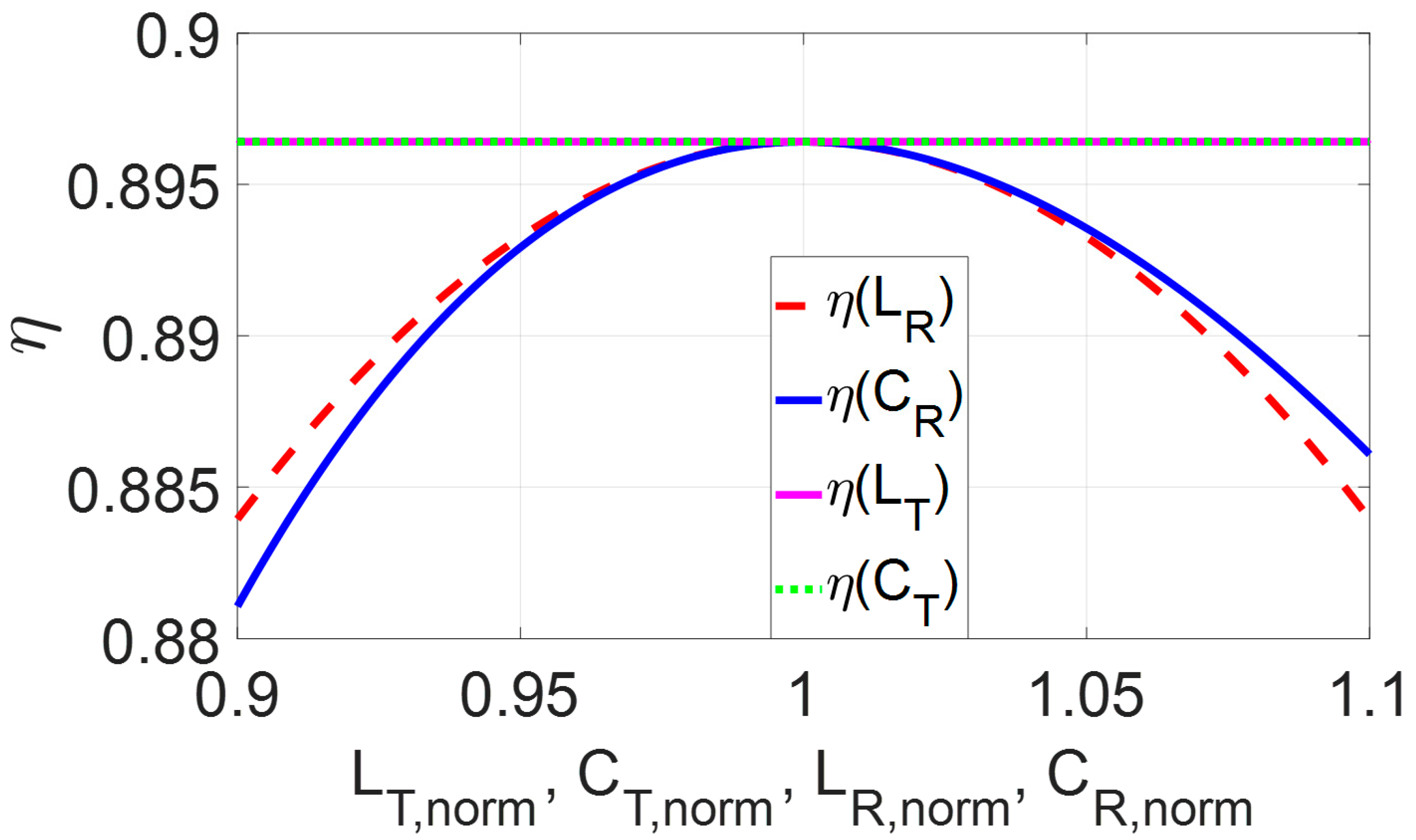
Impact of a frequency mismatch on the IPTS efficiency is exemplified in Figure 3 for a prototypal IPTS used to charge a city-car EV; the designed values of its reactive elements and the supply frequency are listed in

Table 1. IPTS parameter designed values.

Parameter	Symbol	Designed Value
IPTS supply frequency	f	85 kHz
Coupling coil inductances	LT, LR	120 μH
Resonant capacitances	CT, CR	29.2 nF
Series resistances	rT, rR	0.6 Ω
Mutual inductance	M	30 μH
Load	RL	6.1 Ω

together with the load in nominal battery charging conditions [24].

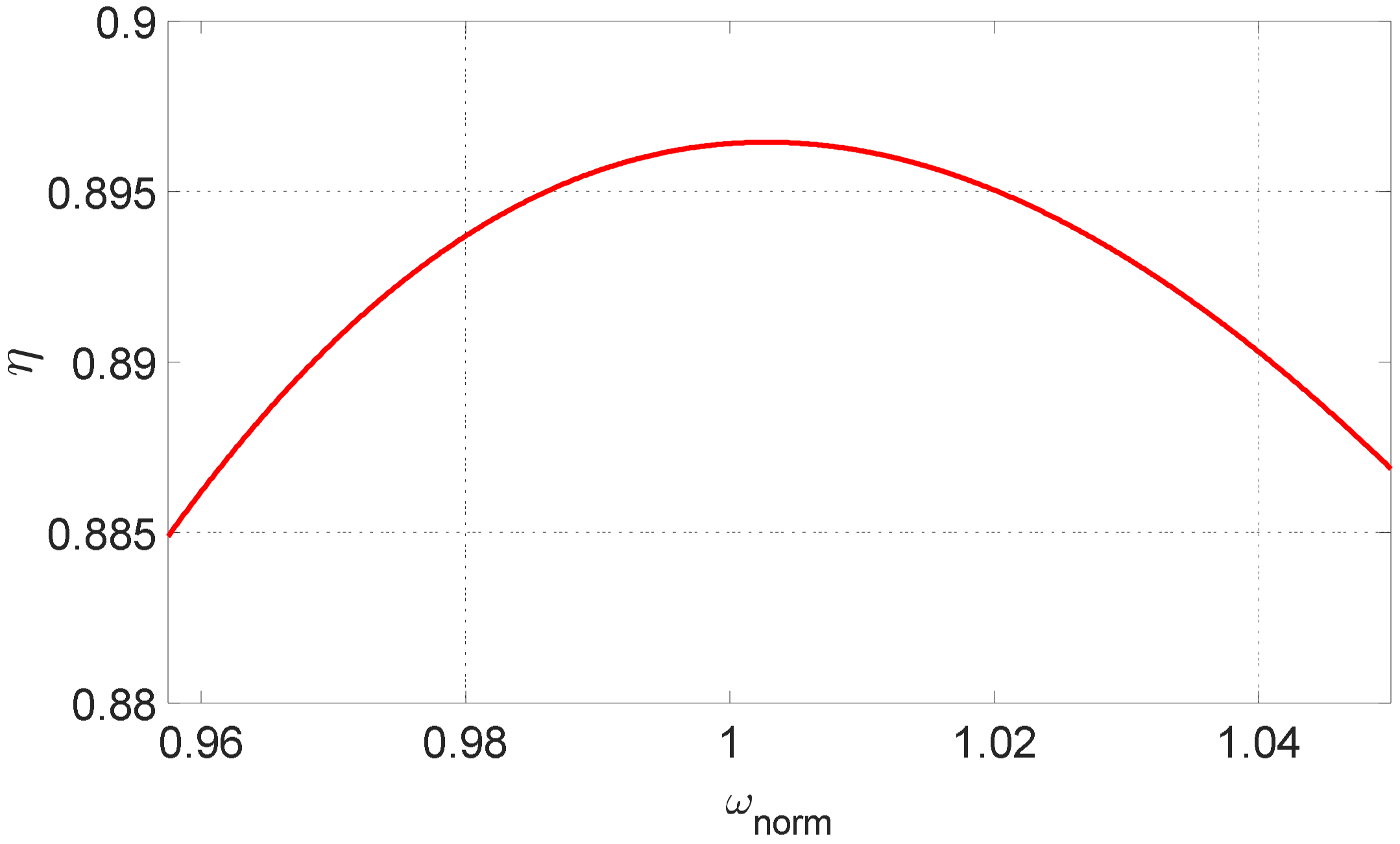
The figure plots four graphs of efficiency, calculated from (8) by varying one at a time L_T, C_T, L_R and C_R and by setting ω at ω₀. In the graphs, the values of the reactive elements range from −10% to +10% of their designed values. For the sake of completeness, Figure 4 plots the graph of efficiency for the reactive elements set at the designed values and for ω varying in the range 81.38 kHz ÷ 90 kHz. The selected ω range follows that set by SAE (Society of Automotive Engineers) RP (Recommended Practice) J2954 for IPTSs projected to charge the battery of EVs. In all graphs, the x-axis is normalized to the design value of the relevant quantity. Inspection of Figure 3 reveals that the impact of L_R and C_R variations, plotted respectively with the red dashed line and the blue solid line, is nearly the same and reduces the efficiency of more than 1% in the worst case. Instead, the L_T and C_T variations, plotted respectively with the horizontal magenta and green dotted lines, do not have any effect on the efficiency. The last outcome is a consequence of (8), where only the real part of ${\dot{Z}}_T$ appears in the expression of the efficiency. Regarding the impact of the ω variations on the efficiency, Figure 4 reveals that the efficiency decreases of about 0.5% at the ends of the spanned ω range and gets its maximum for a ω_norm value a little bigger than 1, in agreement with (16).

Resonance operation can be enforced by tuning the supply frequency but the IPTS ideally resonant operation cannot be reached because, in general, the resonance frequencies of the two stages do not deviate of an equal value. By accounting of the IPTS quantities that can be practically sensed, two tuning methods are envisaged. The first method tunes the supply frequency to make resonant the impedance seen from the inverter output and is hereafter termed as transmitting side resonance (TSR) method. The second one tunes the supply frequency to make resonant the receiving stage, i.e., it sets ω at ω_R, and is hereafter termed as the receiving side resonance (RSR) method.

4.1. TSR Method

The condition to achieve TSR is defined as C1) in Section 3. By (11), the requirement of having v_S,1 in phase to i_T is equivalent to

$$\Im \mathrm{m}\left[{\dot{\mathrm{Z}}}_{\mathrm{T}}+{\dot{\mathrm{Z}}}_{\mathrm{ref}}\right]=0$$

(17)

where $\Im \mathrm{m}\left[·\right]$ is the operator that returns the imaginary part of its argument. By (6) and (7), relation (17) is rewritten in the following polynomial form:

$$\mathrm{P}\left(\mathrm{u}\right)\equiv {\mathrm{A}}_3{\mathrm{u}}^3+{\mathrm{A}}_2{\mathrm{u}}^2+{\mathrm{A}}_1\mathrm{u}+{\mathrm{A}}_0=0$$

(18)

where ω² had been replaced with u and coefficients A₃, A₂, A₁ and A₀ are

$$\left\{\begin{array}{l}{\mathrm{A}}_3={\mathrm{C}}_{\mathrm{T}}{\mathrm{L}}_{\mathrm{R}}{\mathrm{C}}_{\mathrm{R}}^2\left({\mathrm{L}}_{\mathrm{T}}{\mathrm{L}}_{\mathrm{R}}-{\mathrm{M}}^2\right)\hfill \\ {\mathrm{A}}_2=-2{\mathrm{L}}_{\mathrm{T}}{\mathrm{C}}_{\mathrm{T}}{\mathrm{L}}_{\mathrm{R}}{\mathrm{C}}_{\mathrm{R}}-{\mathrm{L}}_{\mathrm{R}}^2{\mathrm{C}}_{\mathrm{R}}^2+{\mathrm{L}}_{\mathrm{T}}{\mathrm{C}}_{\mathrm{T}}{\mathrm{C}}_{\mathrm{R}}^2{\left({\mathrm{r}}_{\mathrm{R}}+{\mathrm{R}}_{\mathrm{L}}\right)}^2+{\mathrm{C}}_{\mathrm{T}}{\mathrm{C}}_{\mathrm{R}}{\mathrm{M}}^2\hfill \\ {\mathrm{A}}_1={\mathrm{L}}_{\mathrm{T}}{\mathrm{C}}_{\mathrm{T}}+2{\mathrm{L}}_{\mathrm{R}}{\mathrm{C}}_{\mathrm{R}}-{\mathrm{C}}_{\mathrm{R}}^2{\left({\mathrm{r}}_{\mathrm{R}}+{\mathrm{R}}_{\mathrm{L}}\right)}^2\hfill \\ {\mathrm{A}}_0=-1\hfill \end{array}\right..$$

(19)

Polynomial P(u) is of third degree and all its coefficients are real. Consequently, P(u) has at least one real solution u₁. Being A₃ > 0 and A₀ < 0, u₁ is positive and a supply angular frequency, denoted with ${\mathsf{\omega }}_{\mathrm{TSR},1}=\sqrt{{\mathrm{u}}_1}$, exists that forces i_T in phase to v_S,1. Moreover, P(u) has other two solutions that if real and positive, give rise to two additional supply angular frequencies that forces i_T in phase to v_S,1, originating the phenomenon known as bifurcation. On the chance that ${\omega }_T={\omega }_R$, paper [25] has set forth the constraints by which the other two solutions are real and positive. Instead, for ${\mathsf{\omega }}_{\mathrm{T}}\ne {\mathsf{\omega }}_{\mathrm{R}}$, the constraints can be found by the Descartes rule of signs. The rule states that if a polynomial has real coefficients and they are sorted by the descending order of the exponent, the number of the real and positive roots is either equal to the number of sign changes between consecutive coefficients or is lower than it by an even number. For P(u) in (18), the other two solutions can exist only if A₂ < 0 and A₁ > 0. Constraint A₁ > 0 requires that

$${\mathrm{R}}_{\mathrm{L}}<{\mathrm{R}}_{\mathrm{L},\mathrm{B}1}\triangleq \sqrt{\frac{2{\mathrm{L}}_{\mathrm{R}}}{{\mathrm{C}}_{\mathrm{R}}}+\frac{{\mathrm{L}}_{\mathrm{T}}{\mathrm{C}}_{\mathrm{T}}}{{\mathrm{C}}_{\mathrm{R}}^2}}-{\mathrm{r}}_{\mathrm{R}}$$

(20)

while constraint A₂ < 0 requires that

$${\mathrm{R}}_{\mathrm{L}}<{\mathrm{R}}_{\mathrm{L},\mathrm{B}2}\triangleq \sqrt{\frac{2{\mathrm{L}}_{\mathrm{R}}}{{\mathrm{C}}_{\mathrm{R}}}+\frac{{\mathrm{L}}_{\mathrm{R}}^2}{{\mathrm{L}}_{\mathrm{T}}{\mathrm{C}}_{\mathrm{T}}}-\frac{{\mathrm{M}}^2}{{\mathrm{L}}_{\mathrm{T}}{\mathrm{C}}_{\mathrm{R}}}}-{\mathrm{r}}_{\mathrm{R}}.$$

(21)

Fulfillment of the constraints is a necessary but not sufficient condition to have bifurcation. However, it can be asserted that i) at low power, i.e., for high values of R_L, IPTS is likely free from bifurcation, and ii) as the power increases, IPTS could be subjected to bifurcation.

Comparison of (20) with (14) reveals that R_L,th is always lower than R_L,B1 while it is lower than R_L,B2 only if

$$1-{\mathrm{k}}^2\frac{{\mathrm{L}}_{\mathrm{T}}{\mathrm{C}}_{\mathrm{T}}}{{\mathrm{L}}_{\mathrm{R}}{\mathrm{C}}_{\mathrm{R}}}>0$$

(22)

where k is the coupling coefficient of the coupler. Because of the low values taken by k in IPTSs, inequality (22) is verified unless the difference between the designed and actual values of the reactive elements gets very high.

Improvement in the efficiency attained with the TSR method has been examined for the prototypal IPTS by taking as supply angular frequency the central solution of (18) whenever bifurcation is detected. The results are plotted in Figure 5 with the same conventions as used in Figure 3. Inspection of the figure outlines that the graphs relevant to the pair L_T, C_T are nearly superimposed such as in Figure 3, but now the same happens also for the pair L_R, C_R. Moreover, the graphs show that efficiency is near to that of IPTS under ideally resonant operation, or even higher when either L_R or C_R goes below their designed values. Instead, a small reduction of the efficiency happens when the loss of resonance is caused by variations of L_T or C_T.

4.2. RSR Method

The condition to achieve RSR is defined as C2) in Section 3. By (5), the requirement of having v_R in phase to i_R is equivalent to

$$\Im \mathrm{m}\left[{\dot{\mathrm{Z}}}_{\mathrm{R}}\right]=0.$$

(23)

Differently from the TSR method, relation (23) leads to an equation that has always one and only one positive solution, given by

$${\mathsf{\omega }}_{\mathrm{RSR}}={\mathsf{\omega }}_{\mathrm{R}}=\frac{1}{\sqrt{{\mathrm{L}}_{\mathrm{R}}{\mathrm{C}}_{\mathrm{R}}}}.$$

(24)

Improvement in the efficiency attained with this tuning method is plotted in Figure 6. The graphs underline that the improvement is like the TSR method when L_R and C_R go lower than the designed values, and even better when they go higher. As (24) is not affected by L_T and C_T, the efficiency remains constant despite the variations of these reactive elements.

5. Phase Control System

Implementation of either of the two methods calls for a phase control system that, acting on the IPTS supply frequency, drives to zero the phase between v_S,1 and i_T, for the TSR method, and the phase between v_R and i_R, for the RSR method. Regarding the implementation of the latter method, it is worth noting that v_R cannot be transduced directly from the terminals of the receiving coil because the voltage between them is comprehensive of the voltage drop across L_R. However, being v_R related to i_T by

$${\overline{\mathrm{V}}}_{\mathrm{R}}=-{\mathrm{j}\mathsf{\omega }\mathrm{M}\overline{\mathrm{I}}}_{\mathrm{T}},$$

(25)

the RSR method is implemented equally well by forcing i_T to lead i_R of π/2.

5.1. Phase Control

The cumulative block diagram of the phase control system for the two methods is shown in Figure 7. In the diagram, the solid-line paths and the variables with no brackets pertain to the block diagram of both TSR and RSR methods. Instead, variables within curly brackets are relevant to the TSR method while those within the square ones to the RSR method.

Phase error θ_err in the diagram is the difference of phase angle reference θ_ref to the actual value θ_act of the controlled phase angle. For the TSR method, θ_ref is equal to zero and θ_act is the phase angle θ_iT,vS between i_T and v_S; for the RSR method, θ_ref is equal to –π/2 and θ_act is the phase angle θ_iT,iR between i_T and i_R. The phase regulator manipulates θ_err and generates reference ω_ref of the IPTS supply angular frequency, which is impressed by the inverter. To protect the phase control system from large errors, phase error θ_err is clamped at [-30°, 30°] before being entered into the regulator.

5.2. Phase Regulator

Specifications for the phase control system are zero phase error at steady state and a reasonably damped behavior. At steady state, the phase relation between the transduced signals depends only on the actual value of ω; hence, the phase regulator must execute an integral action on θ_err for it to reach zero.

By (4), (6) and (7), the phase relations between i_T and v_s,1 at very high and very low supply angular frequency are

$$\left\{\begin{array}{ll}{\left.\frac{{\overline{\mathrm{V}}}_{\mathrm{S},1}}{{\overline{\mathrm{I}}}_{\mathrm{T}}}\right|}_{\mathsf{\omega }\to \infty }\cong {\mathrm{j}\mathsf{\omega }\mathrm{L}}_{\mathrm{T}}\left(1-\frac{{\mathrm{M}}^2}{{\mathrm{L}}_{\mathrm{T}}{\mathrm{L}}_{\mathrm{R}}}\right)\hfill & \underset{⬚}{\Rightarrow }\underset{\mathsf{\omega }\to \infty }{\lim }{\mathsf{\theta }}_{\mathrm{iT},\mathrm{vS}}=-\frac{\mathsf{\pi }}{2}\hfill \\ {\left.\frac{{\overline{\mathrm{V}}}_{\mathrm{S},1}}{{\overline{\mathrm{I}}}_{\mathrm{T}}}\right|}_{\mathsf{\omega }\to 0}\cong \frac{1}{{\mathrm{j}\mathsf{\omega }\mathrm{C}}_{\mathrm{T}}}\hfill & \underset{⬚}{\Rightarrow }\underset{\mathsf{\omega }\to 0}{\lim }{\mathsf{\theta }}_{\mathrm{iT},\mathrm{vS}}=\frac{\mathsf{\pi }}{2}\hfill \end{array}.\right.$$

(26)

By (4), (6) and (25), the phase relations between i_T and i_R under the same situations are

$$\left\{ \begin{array}{l}{\left.\frac{{\overline{\mathrm{I}}}_{\mathrm{R}}}{{\overline{\mathrm{I}}}_{\mathrm{T}}}\right|}_{\mathsf{\omega }\to \infty }\cong -\frac{\mathrm{M}}{{\mathrm{L}}_{\mathrm{R}}}\underset{⬚}{\Rightarrow }\underset{\mathsf{\omega }\to \infty }{\lim }{\mathsf{\theta }}_{\mathrm{iT},\mathrm{iR}}=-\mathsf{\pi }\hfill \\ {\left.\frac{{\overline{\mathrm{I}}}_{\mathrm{R}}}{{\overline{\mathrm{I}}}_{\mathrm{T}}}\right|}_{\mathsf{\omega }\to 0}\cong \frac{1}{{\mathsf{\omega }}^2{\mathrm{MC}}_{\mathrm{R}}}\underset{⬚}{\Rightarrow }\underset{\mathsf{\omega }\to 0}{\lim }{\mathsf{\theta }}_{\mathrm{iT},\mathrm{iR}}=0\hfill \end{array}\right..$$

(27)

For the TSR method, when (18) has only one solution, θ_iT,vS decreases with ω and the gain of the phase regulator must be negative; if bifurcation occurs, an interval of ω exists where θ_iT,vS increases with ω and the gain of the phase regulator must be positive. It follows that the phase regulator must be able to recognize the correct sign for its gain. For the RSR method, this problem does not exist because θ_iT,iR is always a decreasing function of ω and the gain of the phase regulator must be negative.

To comply with the issues of the TSR method, a phase regulator has been synthesized, committed with the task of checking at the beginning of each sampling period if the actual absolute value of the phase error is smaller or greater than that one in the previous sampling period. In the first case, the sign of the gain is maintained while in the second case it is changed before updating ω_ref.

6. Experimental Results

6.1. Experimental Setup

A setup of the phase control system has been arranged according to the TSR method and implemented in the development kit CY8CKIT-059 hosting a programmable system on chip PSoC 5 LC [26], both of Cypress Semiconductor. The setup has been used to tune the supply frequency of the prototypal IPTS pictured in Figure 8. The coupler of the setup is formed by two equal coils that are enclosed in the red plates at the rightmost side of Figure 8. The coils have been designed according to the procedure reported in [27] and have the structure shown in Figure 9. The inverter is built up with a Wolfspeed CCS050M12CM2 SiC MOSFET module [28] and the load is built up with an adjustable resistor emulating a battery with nominal power of 560 W. The PSoC generates the signals to command the inverter switches and a signal proportional to phase error θ_err through an embedded analog-to-digital converter. Quantities v_S and i_T, and the signal proportional to θ_err are acquired by a Tektronix TDS 5034 digital oscilloscope.

6.2. Test Results

The phase control system has been subjected to several tests with different IPTS loads and initial supply frequencies to assess its capabilities in reaching the tuning conditions. In the tests, the magnitude of the inverter output voltage has been kept fixed while its frequency has been changed as dictated by the phase control system. Below, two tests carried out with values of R_L equal to 5.6 Ω and 45 Ω are documented; these R_L values are significant in evaluating the tuning capabilities of the phase control system as the former value does not give rise to any bifurcation while the latter one does it.

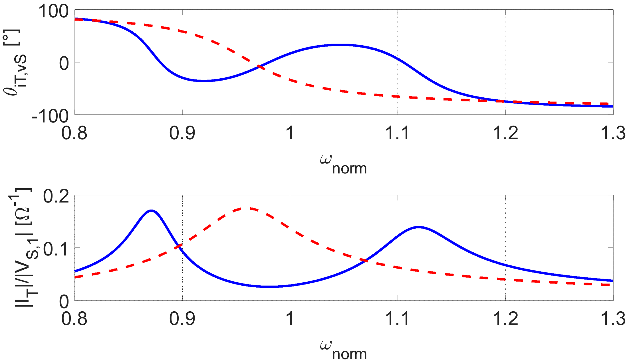
The actual values of the reactive elements of the prototypal IPTS have been measured with an Instek LCR meter model LCR-819 and the resulting values are reported in

Table 2. IPTS parameter actual values.

Parameter	Transmitting Side	Receiving Side
	Actual value	Actual value
Coil inductance	122 μH	119 μH
Resonant capacitance	30.8 nF	30.8 nF
Series resistance	0.7 Ω	0.7 Ω
Mutual inductance	29.5 μH
Coil distance	0.14 m
	Symbol	Value
RL from (14)	RL,th	87.2 Ω
RL from (22)	RL,B1	107.4 Ω
RL from (23)	RL,B2	105.4 Ω

, together with the coils distance and the R_L values in (14), (20) and (21). By substituting these values in the first of (4) and (7), phase θ_iT,vS between i_T and v_S and ratio (28) have been plotted as a function of ω_norm respectively in the upper half and the lower half of Figure 10. Solid and dashed lines in the figure refer respectively to R_L equal to 5.6 Ω and 45 Ω.

$$\frac{\left|{\overline{\mathrm{I}}}_{\mathrm{T}}\right|}{\left|{\overline{\mathrm{V}}}_{\mathrm{S},1}\right|}=\frac{1}{\left|{\dot{\mathrm{Z}}}_{\mathrm{T}}+{\dot{\mathrm{Z}}}_{\mathrm{ref}}\right|}$$

(28)

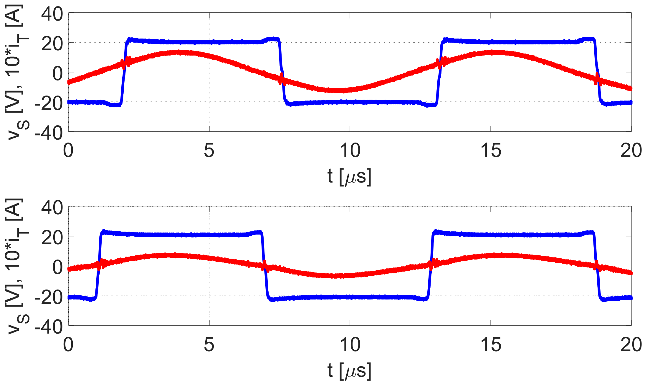
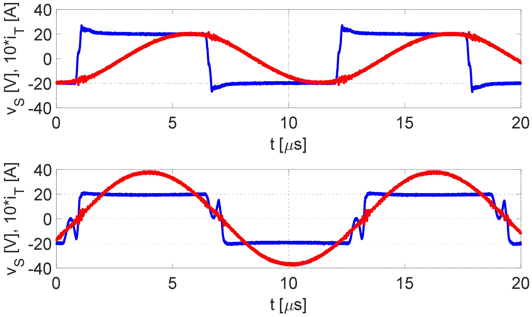
In the test with R_L = 5.6 Ω, the initial supply frequency is set at 89 kHz, i.e., at ω_norm = 1.049, and the corresponding waveforms of v_S and i_T are plotted in the upper half of Figure 11. Processing of the waveforms has resulted in a value of θ_iT,v equal to 27.5°. The waveforms of v_S and i_T at the completion of the tuning process are plotted in the lower half of Figure 11, and the resultant values of ω_norm and θ_iT,vS are 0.997 and 7.7°, respectively. Comparison of the graphs in the two halves of Figure 10 shows that the magnitude of i_T is lower after tuning, although v_s,1 is kept constant. This outcome is substantiated by the solid-line graph in the lower half of Figure 11, which highlights a decrease of $\left|{\overline{\mathrm{I}}}_{\mathrm{T}}\right|/\left|{\overline{\mathrm{V}}}_{\mathrm{S},1}\right|$ for ω_norm moving leftward from the initial value of 1.049.

The behavior of i_T during the tuning process is plotted in the upper half of Figure 12. The solid blue graph, made of more than 4000 supply periods, does not permit to appreciate the waveform of i_T, but confirms that its magnitude decreases about exponentially during the tuning process. The lower half of Figure 12 plots the signal proportional to θ_err. Its behavior shows that the tuning process exhibits a small overshoot and reaches the steady state in about 25 ms.

The test, repeated with R_L = 45 Ω, has led to the graphs in Figure 13 and Figure 14. Now the initial values for ω_norm and θ_iT,vS are respectively 1.048 and −65.5° while, after completion of the tuning process, they are 0.956 and −5.6°. The graphs show that the magnitude of i_T increases after tuning; again, this outcome is substantiated by the dashed-line graph of $\left|{\overline{\mathrm{I}}}_{\mathrm{T}}\right|/\left|{\overline{\mathrm{V}}}_{\mathrm{S},1}\right|$ in the lower half of Figure 9, which highlights an increase of $\left|{\overline{\mathrm{I}}}_{\mathrm{T}}\right|/\left|{\overline{\mathrm{V}}}_{\mathrm{S},1}\right|$ for ω_norm moving leftward from the initial value of 1.049. Here, the steady state is reached in about 25 ms without any overshoot.

The experimental results demonstrate that the TSR method works correctly both with and without bifurcation occurrence and is effective in reducing the phase error between i_T and v_S substantially, even if not exactly to zero. The residual error can be ascribed, at least partially, to the fact that the imposed supply frequency is a submultiple of the clock frequency of PSoC, which does not guarantee the accurate application of the requested frequency.

7. Conclusions

The paper has dealt with the tuning of the supply frequency of IPTSs to improve their efficiency in presence of drifts or tolerances of the reactive elements. After reviewing the impact on the efficiency of the loss of resonance, two methods of tuning the IPTS supply frequency have been examined that impose the resonance condition on either the impedance seen by the transmitting side (TSR) or the receiving side impedance (RSR). Examination of the methods has revealed the occurrence of the bifurcation phenomenon in the TSR method. A phase control system that takes over of the tuning process for both methods has been developed. Implementation of the phase control system in a setup intended to tune the supply frequency of a prototypal IPTS according to the TSR method has been illustrated, together with the countermeasures adopted to face up the bifurcation phenomenon. Finally, the results of experimental tests have been reported to illustrate the tuning capabilities of the method.

References

- Zhang, Z.; Pang, H.; Georgiadis, A.; Cecati, C. Wireless Power Transfer—An Overview. IEEE Trans. on Ind. Electron. 2019, 66, 1011–1058. [Google Scholar] [CrossRef]
- Mi, C.C.; Buja, G.; Choi, S.Y.; Rim, C.T. Modern Advances in Wireless Power Transfer Systems for Roadway Powered Electric Vehicles. IEEE Trans. Ind. Electron. 2016, 63, 6533–6545. [Google Scholar] [CrossRef]
- Mou, X.; Groling, O.; Sun, H. Energy-Efficient and Adaptive Design for Wireless Power Transfer in Electric Vehicles. IEEE Trans. Ind. Electron. 2017, 64, 7250–7260. [Google Scholar] [CrossRef] [Green Version]
- Bosshard, R.; Kolar, J.W. Inductive power transfer for electric vehicle charging: Technical challenges and tradeoffs. IEEE Power Electron. Mag. 2016, 3, 22–30. [Google Scholar] [CrossRef]
- Deng, Q.; Liu, J.; Czarkowski, D.; Hu, W.; Zhou, H. An Inductive Power Transfer System Supplied by a Multiphase Parallel Inverter. IEEE Trans. Ind. Electron. 2017, 64, 7039–7048. [Google Scholar] [CrossRef]
- Jiang, Y.; Wang, L.; Wang, Y.; Liu, J.; Li, X.; Ning, G. Analysis, design and implementation of accurate ZVS angle control for EV’s battery charging in wireless high power transfer. IEEE Trans. Ind. Electron. 2019, 66, 4075–4085. [Google Scholar] [CrossRef]
- Keeling, N.A.; Covic, G.A.; Boys, J.T. A Unity-Power-Factor IPT Pickup for High-Power Applications. IEEE Trans. Ind. Electron. 2010, 57, 744–751. [Google Scholar] [CrossRef]
- Kim, J.-G.; Wei, G.; Kim, M.-H.; Jong, J.-Y.; Zhu, C. A Comprehensive Study on Composite Resonant Circuit-Based Wireless Power Transfer Systems. IEEE Trans. Ind. Electron. 2018, 65, 4670–4680. [Google Scholar] [CrossRef]
- Cabrera, T.; Sánchez, J.A.A.; Longo, M.; Foiadelli, F. Sensitivity analysis of a bidirectional wireless charger for EV. In Proceedings of the 2016 IEEE International Conference on Renewable Energy Research and Applications (ICRERA), Birmingham, UK, 20–23 November 2016; pp. 1113–1116. [Google Scholar]
- Zhang, Y.; Kan, T.; Yan, Z.; Mi, C.C. Frequency and Voltage Tuning of Series–Series Compensated Wireless Power Transfer System to Sustain Rated Power Under Various Conditions. IEEE J. Emerg. Sel. Top. Power Electron. 2019, 7, 1311–1317. [Google Scholar] [CrossRef]
- Shin, J.; Outeiro, M.T.; Czarkowski, D. New real-time tuning method for wireless power transfer systems. In Proceedings of the IEEE Wireless Power Transfer Conference (WPTC), Aveiro, Portugal, 5–6 May 2016; pp. 1–4. [Google Scholar]
- Sasatani, T.; Narusue, Y.; Kawahara, Y.; Asami, T. DC-based impedance tuning method using magnetic saturation for wireless power transfer. In Proceedings of the IEEE Wireless Power Transfer Conference (WPTC), Taipei, Taiwan, 10–20 May 2017; pp. 1–4. [Google Scholar]
- Saltanovs, R. Multi-capacitor circuit application for the wireless energy transmission system coils resonant frequency adjustment. In Proceedings of the IEEE Wireless Power Transfer Conference (WPTC), Boulder, CO, USA, 13–15 May 2015. [Google Scholar]
- Baikova, E.N.; Baikov, A.V.; Valtchev, S.; Melicio, R. Frequency Tuning of the Resonant Wireless Energy Transfer System. In Proceedings of the 45th Annual Conference of the IEEE Industrial Electronics Society (IECON), Lisbon, Portugal, 14–17 October 2019. [Google Scholar]
- Xia, J.; Chen, D.; Wang, D.; Xu, D. Analysis of Automatic Frequency Tuning for Wireless Power Transfer Systems. In Proceedings of the IEEE 4th Advanced Information Technology, Electronic and Automation Control Conference (IAEAC), Chengdu, China, 20–22 December 2019. [Google Scholar]
- Sis, S.A.; Bicakci, S. A resonance frequency tracker and source frequency tuner for inductively coupled wireless power transfer systems. In Proceedings of the 46th European Microwave Conference (EuMC), London, UK, 4–6 October 2016; pp. 751–754. [Google Scholar]
- Kar, D.P.; Nayak, P.P.; Bhuyan, S.; Panda, S.K. Automatic frequency tuning wireless charging system for enhancement of efficiency. Electron. Lett. 2014, 50, 1868–1870. [Google Scholar] [CrossRef]
- Wang, C.-S.; Covic, G.A.; Stielau, O.H. Power transfer capability and bifurcation phenomena of loosely coupled inductive power transfer systems. IEEE Trans. Ind. Electron. 2004, 51, 148–157. [Google Scholar] [CrossRef]
- Chopra, S.; Bauer, P. Analysis and design considerations for a contactless power transfer system. In Proceedings of the IEEE 33rd International Telecommunications Energy Conference (INTELEC), Amsterdam, The Netherlands, 9–13 October 2011. [Google Scholar]
- Villa, J.L.; Sallan, J.; Sanz Osorio, J.F.; Llombart, A. High-Misalignment Tolerant Compensation Topology For ICPT Systems. IEEE Trans. Ind. Electron. 2012, 59, 945–951. [Google Scholar] [CrossRef]
- Sohn, Y.H.; Choi, B.H.; Lee, E.S.; Lim, G.C.; Cho, G.H.; Rim, C.T. General Unified Analyses of Two-Capacitor Inductive Power Transfer Systems: Equivalence of Current-Source SS and SP Compensations. IEEE Trans. Power Electron. 2015, 30, 6030–6045. [Google Scholar] [CrossRef]
- Qu, X.; Jing, Y.; Han, H.; Wong, S.C.; Tse, C.K. Higher Order Compensation for Inductive-Power-Transfer Converters With Constant-Voltage or Constant-Current Output Combating Transformer Parameter Constraints. IEEE Trans. Power Electron. 2017, 32, 394–405. [Google Scholar] [CrossRef]
- Aditya, K.; Williamson, S.S. A Review of Optimal Conditions for Achieving Maximum Power Output and Maximum Efficiency for a Series–Series Resonant Inductive Link. IEEE Trans. Transport. Electrific. 2017, 3, 303–311. [Google Scholar] [CrossRef]
- Buja, G.; Bertoluzzo, M.; Mude, K.N. Design and experimentation of IPT charger for electric city car. IEEE Trans. Ind. Electron. 2015, 62, 7436–7447. [Google Scholar] [CrossRef]
- Aditya, K.; Williamson, S.S. Design Guidelines to Avoid Bifurcation in a Series-Series Compensated Inductive Power Transfer System. IEEE Trans. Ind. Electron. 2019, 66, 3973–3982. [Google Scholar] [CrossRef]
- CY8CKIT-059 PSoC 5LP Prototyping Kit Guide. Available online: http://http://www.cypress.com/file/157971/download, (accessed on 21 February 2020).
- Mude, K.N.; Bertoluzzo, M.; Buja, G.; Pinto, R. Design and experimentation of two-coil coupling for electric city-car WPT charging. J. Electromagn. Waves Appl. 2016, 30, 70–88. [Google Scholar] [CrossRef]
- CCS050M12CM2 1.2kV, 25mΩ All-Silicon Carbide Six-Pack (Three Phase) Module. Available online: https://www.wolfspeed.com/ccs050m12cm2, (accessed on 21 February 2020).
Figure 1.
Scheme of SS-compensated IPTS.
Figure 2.
Circuital representation of SS-compensated IPTS.
Figure 3.
Efficiency under IPTS non-ideal resonant operation due to variation of the reactance of the coils or of the resonant capacitors.
Figure 4.
Efficiency under IPTS non-ideal resonant operation due to variation of the supply angular frequency.
Figure 5.
Efficiency improvement by TSR method.
Figure 6.
Efficiency improvement by RSR method.
Figure 7.
Block diagram of the phase control system.
Figure 8.
Phase control system setup and prototypal IPTS.
Figure 9.
Coil without protective cover.
Figure 10.
Phase angle θiT,vS (up) and ratio (down) vs. ωnorm for RL = 5.6 Ω (blue solid line) and RL = 45 Ω (red dashed line).
Figure 11.
Inverter output voltage (blue line) and current (red line) before (up) and after (down) tuning with RL = 5.6 Ω.
Figure 12.
Transmitting coil current (up) and phase error (down) during tuning with RL = 5.6 Ω.
Figure 13.
Inverter output voltage (blue line) and current (red line) before (up) and after (down) tuning with RL = 45 Ω.
Figure 14.
Transmitting coil current (up) and phase error (down) during tuning with RL = 45 Ω.