Relativistic Configuration-Interaction and Perturbation Theory Calculations for Heavy Atoms

Abstract

Heavy atoms present challenges to atomic theory calculations due to the large number of electrons and their complicated interactions. Conventional approaches such as calculations based on Cowan’s code are limited and require a large number of parameters for energy agreement. One promising approach is relativistic configuration-interaction and many-body perturbation theory (CI-MBPT) methods. We present CI-MBPT results for various atomic systems where this approach can lead to reasonable agreement: La I, La II, Th I, Th II, U I, Pu II. Among atomic properties, energies, g-factors, electric dipole moments, lifetimes, hyperfine structure constants, and isotopic shifts are discussed. While in La I and La II accuracy for transitions is better than that obtained with other methods, more work is needed for actinides.

1. Introduction

Heavy atoms, such as actinides, are highly challenging for atomic calculations for at least the following reasons: (1) most actinides and lanthanides have many valence electrons, including f-electrons, and hence a large number of closely spaced fine-structure states. Together with a significant configuration mixing, this leads to difficulties in identification of states and accurate calculations of properties that depend on configurations and terms. To achieve adequate accuracy, all-order methods, such as configuration-interaction (CI) methods, are needed to account for valence-valence interactions. (2) The valence electrons strongly interact with a large number of core electrons. This interaction cannot be ignored and needs to be treated beyond the second order in many-body perturbation theory (MBPT), if the calculations are carried out in the CI-MBPT framework. Here, several options exist for improvement of accuracy: scaling second-order MBPT corrections [1,2,3], including higher-order effects as in CI-all-order approach [4,5], or including upper core electrons into the valence space [6]. (3) Relativistic effects are significant and lead to deviation from the LS coupling scheme. Because, for example, electric-dipole transitions conserve the total spin in non-relativistic approximation, the mixing of states of different S has a strong effect on the magnitude of the electric dipole transitions and is one reason for large uncertainty in the computed values. Codes, such as Cowan’s popular code, treat relativistic effects quite approximately, for example, by including spin-orbit terms but neglecting many other important terms. To amend this, generalization lead to relativistic analogs of Cowan’s code, such as the Los Alamos suite of relativistic atomic physics codes [7]. Even relativistic MBPT approach, which is based on the Dirac–Hartree–Fock (DHF) starting potential, does not include a number of significant relativistic effects beyond DHF.

In the case of actinides, the experimental data are limited owing to difficulties of dealing with radioactive atoms. Uranium, with the relatively stable isotope U-238, is extensively studied because of its roles in global security [8,9,10], atomic energy [11], and more. The spectroscopy of the uranium atom can be used for detection and characterization of its isotopic content for nuclear forensics [8,9,10] and treaty monitoring. Uranium isotopes are also of interest for measuring the stellar ages [12]. While many energy levels were identified and their energy accurately measured [13], transition rates or oscillator strengths were not yet reliably determined. Similar spectroscopic data were also acquired for the related element plutonium [14,15]. More generally, additional motivations for studying actinides include nuclear chronometry in astrophysics and the search for a nuclear clock transitions in thorium.

The method of valence-valence CI with all-order valence-core corrections was used by Safronova et al. [4] to calculate energies of Th I, Th II, and Th III, but unfortunately transition probabilities or lifetimes for Th II were not presented. The CI-all order approach is a method to include valence-core interaction beyond the second order in an ab initio way. This can be necessary when experimental energies are not available, e.g., in super heavy atoms. The CI-all order approach is quite promising, but it requires massive computer resources and is noticeably slower than simpler models. The starting point for this approach is that in single-valence atoms, like Fr I, a good accuracy was achieved by including single-double excitations.

Th II has also been investigated using CI and CI-MBPT approaches. Flambaum and Dzuba [16] showed that the number of states in Th II, as well as in Th I, grows exponentially with the energy of the states, which is a useful property for nuclear clocks, while it also indicates the complexity of the spectrum, making the precise calculations difficult. Another study showed that a nuclear clock transition with Th II can be enhanced through the electronic bridge process [17].

In many applications, transition probabilities are of great interest and they are also valuable for testing theories. A large compilation of transition probability data for 70 elements, including uranium and thorium, is given in [18].

2. CI-MBPT Framework

The CI-MBPT framework is convenient for the analysis of complex atoms. The main idea is to divide all atomic electrons into two groups: valence electrons and core electrons. This is quite natural for atoms because the valence electrons have much smaller binding energy than core electrons, and the interaction between core and valence electrons is much weaker than between valence electrons. CI-MBPT can both accurately treat valence-valence interactions via CI and efficiently treat valence-core interactions via MBPT. In general, the required size of the CI matrix scales exponentially with the number of included electrons, while MBPT scales much slower with the number of considered valence and core electrons. This scaling depends on the number of excited core electrons, and in many cases single- and double-core excitations are most important. Unfortunately, in the case of heavy atoms, valence electrons start to interact considerably with the core electrons, and ab initio second-order MBPT is not sufficient to reproduce fine structure splittings. Thus, some modifications (parametric CI-MBPT, e.g.,) are needed, which will be discussed below.

2.1. CI-MBPT Formalism

To calculate energies and wavefunctions, a CI-MBPT method developed for open shell atoms with multiple valence electrons described in, e.g., [19] can be used. The effective CI-MBPT Hamiltonian for an atom is split into two parts:

$$H^{eff}=\sum _{i=1}^M{h}_{1i}+\sum _{i\ne j}^M{h}_{2ij}.$$

(1)

In addition to the $V^{N-M}$ DHF potential, the one-electron contribution

$$h_1=c\mathbf{\alpha }·\mathbf{p}+(\beta -1)m{c}^2-Z{e}^2/r+V^{N-M}+{\Sigma }_1$$

(2)

contains the valence electron self-energy correction, ${\Sigma }_1$ [20]. Here, c is the speed of light, m is the electron mass, Z is the nuclear charge, $\alpha$ and $\beta$ are matrices encountered in Dirac’s equation. In the CI-MBPT program, the self-energy correction ${\Sigma }_1$ is calculated with the second-order MBPT. It can be scaled with nine factors for one-electron relativistic angular momentum numbers: $s_{1/2}$, $p_{1/2}$, $p_{3/2}$, $d_{3/2}$, $d_{5/2}$,$f_{5/2}$, $f_{7/2}$, $g_{7/2}$, and $g_{9/2}$. These factors when different from unity take into account both many high-order MBPT corrections and relativistic effects, including the one-particle Hartree–Fock–Breit term, which also can be included in the CI-MBPT program. The two-electron Hamiltonian is

$$h_2=e^2/|{\mathbf{r}}_{\mathbf{1}}-{\mathbf{r}}_{\mathbf{2}}|+{\Sigma }_2$$

(3)

where ${\Sigma }_2$ is the Coulomb interaction screening term arising from the presence of the core [21], which is calculated in the second order by MBPT. Fitting with additional scaling factors was introduced for zero-, first-, and beyond-order multipolarity of the Coulomb interaction. Further details on the CI-MBPT approach can be found in ref. [22].

2.2. CI-MBPT Numerical Procedure

For numerical calculations, firstly, the V${}^{N-M}$ DHF potential is calculated. The number of removed electrons M can be chosen by the user. When all valence electrons are removed, it is the most theoretically consistent starting potential, but not the most optimal because with smaller M the starting potential is closer to the physical potential to give the best single-electron approximation, but the subtraction-diagram MBPT terms were not programmed. The potential when the valence electrons are included is symmetrized by assuming a spherically symmetric closed shell with a scaling factor introduced to take into account the actual number of valence electrons. For example, $d^3$ would be a 0.3 portion of a spherically symmetric $d^{10}$ potential. This scaling factor is not included into the optimization procedure and is fixed by the number of valence electrons included into the starting potential.

Secondly, the basis in the frozen V${}^{N-M}$ potential is calculated using a B-spline subroutine, with a cavity of some radius R chosen for the ion or the atom: $R\approx 30/(Z+1)$ where Z is the positive charge of an ion, and zero for a neutral atom. For example for U I CI-MBPT calculations, R can be chosen 30 a.u. In this basis, the CI-MBPT terms of Equation (1) are evaluated. The final step in the calculation of energy states and wavefunctions is the solution of eigenvalue problem for the effective Hamiltonian matrix.

The program can generate a set of configurations for single-, double-, etc. excitations of the input configurations limited by a given maximum angular momentum $l_{max}$ and principle number $N_{max}$. Alternatively, a list of nonrelativistic input configurations can be given that includes the dominant configurations, and no or fewer excitations can be used. The effective Hamiltonian matrix generation is repeated multiple times for different scaling factors (in the parametric CI-MBPT method) and an optimization procedure described below is used until some optimum is reached. For the matrix element evaluation, random-phase approximation (RPA) corrections are added to take into account core-polarization effects.

2.3. Ab Initio CI-MBPT

In ab initio CI-MBPT, the scaling MBPT coefficients are set to one. It works well for light atoms, which have valence-core interactions sufficiently small that they can be taken into account in the second order of MBPT. For example, Si I ab initio CI-MBPT calculations resulted in close agreement with experiment for energies and transition probabilities [23,24]. Good agreement is also found in CI-MBPT calculations for Ge, Sn, and Pb [19], although the level of accuracy is decreased. An additional problem for CI-MBPT is that the starting potential can be insufficiently accurate and the convergence of CI is too slow. CI-MBPT has reasonable accuracy for four-valence-electron atoms, but if an atom has more, the number of determinants becomes too large, so a more efficient starting potential is needed which includes some valence electrons, as described in the next subsection.

2.4. Ab Initio Relativistic CI

When many valence electrons are present, for example in case of U I, it is difficult to saturate the basis using closed-shell starting potential for which CI-MBPT was consistently developed. The most efficient way to achieve fast convergence is to include almost all valence electrons into the starting potential. This will result in a set of states that for lowest-energy states can be described by almost pure configurations. Moreover, the excitation over principle quantum numbers does not need to be high in relativistic CI (RCI), and small-size basis sets can be quite adequate for low-energy states.

One issue is that not all states can be well approximated with a single starting potential. For example, U I $5f^{3}6d7s^2$ and $5f^{3}6d^{2}7s$ states have different optimal starting potentials. When the state is pure, then one potential can be chosen for this state to calculate its property, but when the states are mixed or when a transition needs to be calculated, some compromise is needed. For example, a transition from the ground state J = 6 $5f^{3}6d7s^2$ to J = 5 $5f^{3}6d7s7p$ can be calculated using the $V^{N-1}$$5f^{3}7s^2$ potential, which at least for $7s$ and $7p$ electrons give the effective charge +1. For technical reasons, the CI-MBPT program used did not allow a $5f^{3}6d7s$ starting potential. Another possibility is a $5f^4$ starting potential with charge +2 for U I electrons. In both cases, because the starting potentials are not ideal, the RCI basis set needs to include higher n to correct the radial functions. For example, the configurations $5f^{3}6d7s8s$, $5f^{3}7d7s^2$, and $5f^{2}6f6d7s^2$ can be included. This RCI method was tested in hyperfine constant calculations of U I, and good agreement was obtained [25].

2.5. Parametric CI-MBPT

Parametric CI-MBPT can improve the accuracy of ab initio CI-MBPT to match theoretical and experimental energies, and hence, facilitate the identification of the states. In heavy atoms, this approach is useful, especially for highly excited states.

The main challenge is that optimization of the parameters requires a large number of CI-MBPT calculations. Depending on the size of the Hamiltonian matrix, this can take a long time. Various optimization algorithms can be used, but in general they have to be efficient. Below are examples of parametric CI-MBPT calculations.

2.5.1. Energies of Even Th I States

The first test of actinides by parametric CI-MBPT was done for Th I atom. This atom is relatively regular and the spectroscopic database is detailed. Th I is important for various applications and the Th I spectrum is used for the calibration purpose. CI-MBPT calculations were carried out using a $V^{N-4}$ starting potential. The interaction of four valence electrons were accounted with CI with the basis set. The configuration set started with basic configurations such $6d^{2}7s^2$, $6d^{3}7s$, $5f7s^{2}7p$, $6d^4$, $5f6d7s7p$, and included the lowest single excitations: $6d^{2}7s8s$, etc. Single and double excitations from these listed nonrelativistic configurations were also allowed to 8s,8p,7d,6f. The optimization of the parameters was done with the following simple algorithm: (1) a minimum was determined for the first parameter; (2) its value was substituted and the minimum was determined for the second parameter; (3) the procedure was repeated until all nine parameters were optimized in sequence; (4) their values were substituted and the steps 1–3 were repeated until the changes in the energy deviations became small. This algorithm was not very efficient and required repetition of CI-MBPT calculations in sequence for many hours.

A large number of Th I even states were calculated with parametric CI-MBPT [1]. With nine adjustable parameters, 7 for single-electron self energy and 2 for Coulomb screening, an agreement of 100–200 cm${}^{-1}$ was achieved for 16 levels for each J = 1 to 6. Furthermore, the agreement for g-factors was also close for the first 7 states of each J. However, higher-energy levels were less consistent, which is expected for the limited number of the parameters used. Also, compared to CI-all-order method [4], the agreement between theory and experiment is similar.

2.5.2. Energies and Transitions of La II and La I

La II is particularly interesting for the parametric CI-MBPT because the CI part for 2 valence electrons can be easily saturated and the main focus can be placed on the valence-core interaction. In La II parametric CI-MBPT calculations [2], parameters were adjusted to improve the accuracy of the valence-core interaction beyond second-order MBPT. For optimization of ${\Sigma }_2$ parameters first and some reoptimization of some ${\Sigma }_1$ and ${\Sigma }_2$ parameters, the particle swarm method [26,27] was used. This method has an advantage that it can accelerate the optimization by engaging multiple computer cores.

The crucial test was to calculate transition matrix elements, which often present difficulties for semi-empirical calculations. If the model correctly describes physics, transition matrix elements will be reproduced well. The parametric CI-MBPT of [2] indeed accounted accurately for valence-core interaction, leading to a consistent agreement for electric-dipole transition probabilities for a large number of transitions. In fact, the accuracy was systematically better than of a previous parametric theory based on Cowan code with core-polarization corrections [28].

Although La I is quite similar to La II in terms of valence-core interactions, calculations of La I transitions are more challenging [3]. There are many cases of closely spaced levels of the same symmetry which are strongly mixed. A special method was applied to improve accuracy for matrix elements of strongly mixed states, which lead to consistent agreement between theory and experiment for a large number of transitions and lifetimes. Other calculations, such as relativistic Hartree–Fock (the approach of Cowan’s code) with core-polarization HFR+CP [29] and multiconfiguration Hartree–Fock with Breit-Pauli correction (MCHF+BP) [30] gave less accurate results. The analysis of theoretical accuracy was introduced based on uncertainties of optimized parameters and mixing angles [3]. The theoretical error bars were consistent with experimental errors, validating the method.

2.5.3. Lifetimes of Th II

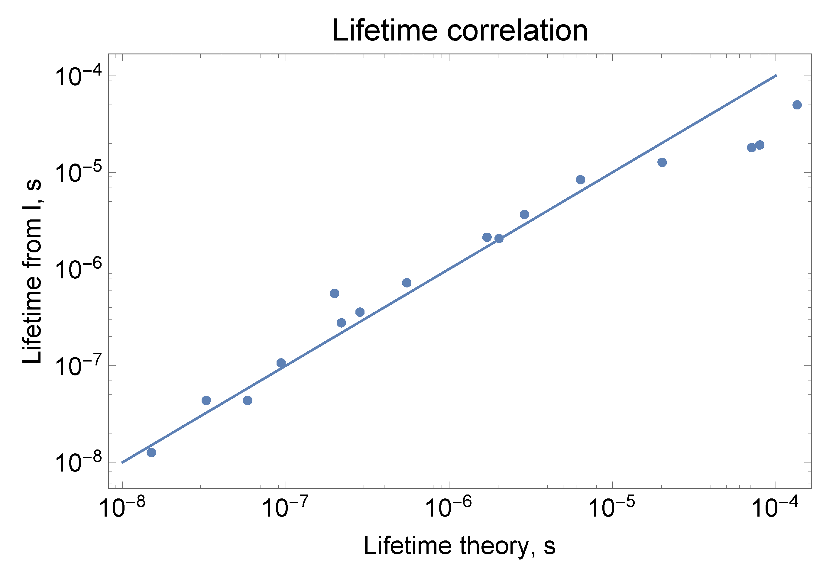
Many transition oscillator strengths and lifetimes of Th II were measured [31,32,33,34]. Some uses include cosmological applications [35], nuclear clocks [36], and calibration standards [37]. While the Th II ion is an analog of the La I atom, with three valence electrons above the core, Th II transition lifetime calculations have significant uncertainty [38]. One reason for this is strong mixing between three or more states. This becomes evident because after averaging over the mixed states, theoretical lifetimes start to agree well with the experimental values (Figure 1). Another useful conclusion from the work was that experimental intensities given by NIST for Th II can be used in conjunction with theory to obtain lifetimes. Many lifetimes of low-energy levels, for which theory is more reliable, were not measured, so this method can provide additional lifetime data. With the help of local thermal equilibrium (LTE) approximation, level populations for different levels can be related, so only one proportionality coefficient k and one temperature T are needed to obtain the radiative decay rates $A_i^{exp,I}$ for different levels i from normalized intensities $I_{i,j}$:

$$A_i^{exp,I}=k\sum _j{I}_{ij}{e}^{E_i/T}.$$

(4)

Radiative decay rates are related to lifetimes, ${\tau }_i=1/A_i$. Figure 1 shows the fit, which for the most part is quite close to the experimental points. From the fit, lifetime values were listed in [38] for J = 2.5 odd states:

$${\tau }_i^{exp,I}=1/(k\sum _j{I}_{ij}{e}^{E_i/T}).$$

(5)

The fitting parameters k and T can be found from comparison with theoretical lifetimes,

$${\tau }_i^{Th}=1/(\sum _j{A}_{ij}^{Th}),$$

(6)

to obtain the experimental intensity-derived lifetimes. A similar analysis was performed for J = 1.5 odd states.

2.5.4. U I

The neutral uranium atom (U I) is of significant interest owing to important applications, such as detection of uranium and characterization of its isotopic content. This atom has six valence electrons and is difficult even for approximate calculations. Parametric CI-MBPT or parametric RCI (pRCI) can be used to get some agreement of energies, g-factors, configuration assignment, and hyperfine constants. Here, U I calculations are presented in some detail.

Table 1. Energies (in cm${}^{-1}$ from the lowest presented level) and other properties of U I odd J = 7 states. Calculations are performed with (parametric) pCI-MBPT and pRCI methods described here. Configuration A: $5f^{3}6d7sns(n=7\dots 10)+5f^{3}nd7s^2(n=6\dots 11)+5f^{2}6f6d7s^2+5f^{3}6d^{2}7s$; Configuration B: $5f^{3}6d7s^2,5f^{3}6d7s8s,5f^{3}7d7s^2,5f^{2}6f6d7s^2,5f^{3}6d^{2}7s,5f^{3}6d^{2}8s,5f^{3}6d7d7s,5f^{2}6f6d^{2}7s$; Configuration C: $5f^{3}6d7s^2,5f^{3}6d7s8s,5f^{3}6d8s^2,5f^{3}7d7s^2,5f^{3}7d7s8s,5f^{3}6d^{2}7s,5f^{3}6d^{2}8s,5f^{3}6d7d7s,5f^{3}6d7d8s,5f^{2}6f6d^{2}7s$. Conf.DB are configuration notations taken from Data Base [13], and Conf.th are configurations obtained by CI-MBPT; g is Landé g-factor from Data Base [13]. $B_{HFS}$(th) and $B_{HFS}$(expt) are current CI-MBPT and experimental [39] quadrupole hyperfine constants (in MHz), respectively.

Potential	Coeff.: $s_{1/2},p_{1/2},d_{3/2},d_{5/2}$
	$f_{5/2},f_{7/2}$, L = 0, L = 1
$V^{N-2}5f^4$ A	−0.0478, 0.0000, 0.4770, 0.0000, 0.6547
	0.0000, 0.0903, 0.9506, 1.3276, 0.6
Conf.DB	Conf.th	$E_{th.}$	$E_{expt.}$	$\Delta E$	g	$\Delta g\times {10}^4$	$B_{HFS}\left(th\right)$	$B_{HFS}\left(expt\right)$
$d{s}^2$	$d{s}^2$	0	0	0	0.925	22	4485	4112
$d{s}^2$	$d{s}^2$	3528	3525	3	1.020	16	1363	1239
$d^{2}s$	$d^{2}s$	4336	4317	19	0.845	5	1661	2412
$d{s}^2$	$d^{2}s$	6274	6268	5	0.930	94	791	2744
$d{s}^2$	$d{s}^2$	7791	7876	−85	1.095	−132	2861
$d^{2}s$	$d^{2}s$	9081	9025	56	0.890	206	181
$d^{2}s$	$d{s}^2$	9435	9546	−111	0.985	171	−297
$d{s}^2$	$d{s}^2$	9919	9767	151	1.010	19	2115
Potential	Coeff.: $s_{1/2},p_{1/2},d_{3/2},d_{5/2}$
	$f_{5/2},f_{7/2}$, L = 0, L = 1
$V^{N-2}5f^4$ A	−0.0602, 0.0000, 0.1, 0.0000, 0.2756
	0.0000, 0.0904, 0.9868, 1.4277, 1.7654
Conf.DB	Conf.th	$E_{th.}$	$E_{expt.}$	$\Delta E$	g	$\Delta g\times {10}^4$	$B_{HFS}$
$d{s}^2$	$d{s}^2$	0	0	0	0.925	3	4578	4122
$d{s}^2$	$d{s}^2$	3692	3525	167	1.020	27	1089	1239
$d^{2}s$	$d^{2}s$	4359	4317	42	0.845	−28	1817	2412
$d{s}^2$	$d{s}^2$	6745	6268	477	0.930	22	3163	2744
$d{s}^2$	$d^{2}s$	7619	7876	−258	1.095	−99	1079
$d^{2}s$	$d{s}^2$	8742	9025	−283	0.890	228	762
$d^{2}s$	$d{s}^2$	9542	9546	−4	0.985	138	377
$d{s}^2$	$d^{2}s$	10,029	9767	262	1.010	98	230
Potential	Coeff.: $s_{1/2},p_{1/2},d_{3/2},d_{5/2}$
	$f_{5/2},f_{7/2}$, L = 0, L = 1
$V^{N-2}5f^4$ B	1.8799, 0.1266, 0.4544, 0.2025, 0.4492
	0.0000, 0.1094, 1.0078, 1.4146, 0.6032
Conf.DB	Conf.th	$E_{th.}$	$E_{expt.}$	$\Delta E$	g	$\Delta g\times {10}^4$	$B_{HFS}$
$d{s}^2$	$d{s}^2$	0	0	0	0.925	0	3543	4122
$d{s}^2$	$d{s}^2$	3185	3525	−341	1.020	27	1210	1239
$d^{2}s$	$d^{2}s$	4516	4317	198	0.845	−32	2024	2412
$d{s}^2$	$d{s}^2$	6681	6268	412	0.930	−14	3151	2744
$d{s}^2$	$d{s}^2$	7747	7876	−130	1.095	42	211
$d^{2}s$	$d^{2}s$	8238	9025	−788	0.890	95	1351
$d^{2}s$	$d{s}^2$	9661	9546	115	0.985	106	604
$d{s}^2$	$d^{2}s$	10,378	9767	610	1.010	93	192
Potential	Coeff.: $s_{1/2},p_{1/2},d_{3/2},d_{5/2}$
	$f_{5/2},f_{7/2}$, L = 0, L = 1
$V^{N-6}$ C	0.5522, 0.6029, 0.6583, 0.8514, 0.7550
	0.9406, 1.0139, 1.0460, 1.2340, 0.9068
Conf.DB	Conf.th	$E_{th.}$	$E_{expt.}$	$\Delta E$	g	$\Delta g\times {10}^4$	$B_{HFS}$
$d{s}^2$	$d{s}^2$	0	0	0	0.925	−10	4100	4122
$d{s}^2$	$d{s}^2$	2827	3525	−699	1.02	30	1355	1239
$d^{2}s$	$d^{2}s$	4246	4317	−72	0.845	−33	2855	2412
$d{s}^2$	$d{s}^2$	6516	6268	248	0.93	198	694	2744
$d{s}^2$	$d{s}^2$	7410	7876	−466	1.095	−187	3487
$d^{2}s$	$d{s}^2$	8734	9025	−291	0.89	300	228
$d^{2}s$	$d^{2}s$	9620	9546	74	0.985	−18	1907
$d{s}^2$	$d{s}^2$	10,263	9767	496	1.01	88	990

shows a comparison of several methods for eight U I J = 7 odd states: (1) the $V^{(N-2)}5f^4$ DHF starting potential with configurations A defined in the table caption and one set of 7 optimized parameters; (2) the same starting potential and configurations but with another set of 7 optimized parameters; (3) the same starting potential but different configurations B; (4) parametric CI-MBPT with $V^{N-6}$ starting potential (valence electrons removed) and 10 fitting parameters. It is expected that a $V^{N-2}$ starting potential is better than $V^{N-6}$, and this can be clearly seen from much better agreement for energies of cases 1–3 over case 4. For example, case 1 has energy differences smaller than 100 cm${}^{-1}$ for the first six states, while case 4 has even the second state inaccurate by 699 cm${}^{-1}$, despite many more fitting parameters being used in case 4. The case 1 model is quite similar to the models of cases 2 and 3, but the case 1 model has more configurations than case 3, A vs. B, and also, case 2 has a larger deviation of parameters from zero. Zero parameters mean ab initio RCI, and nonzero coefficients do not have physical meaning except that they approximately take into account MBPT corrections and valence–valence interactions beyond those represented in the model space.

Within the $V^{N-2}5f^4$ starting potential, cases 2 and 3 have better agreement of quadrupole hyperfine constants for the first four J = 7 odd states, while case 1 has states 4 and 5 exchanged. The same is true for case 4. The quadrupole instead of dipole constant is chosen due to better stability of the quadrupole constant with the variation of parameters. Thus even though energies and g-factors are accurate in case 1, the quadrupole constant indicates the state reversal. The probability of reversal or mixing increases with the state energy.

To check the behavior for states of higher energies, one additional calculation was performed for 20 J = 6 even levels in $V^{N-2}5f^4$ potential with 10 optimized parameters.

Table 2. Comparison of parametric RCI (pRCI) configurations, energies, and g-factors with ones given in database (DB) [13] for 20 J = 6 odd U I states. pRCI parameters are the following: potential: $V^{N-2},5f^4$; configurations: $5f^{3}6d7s^2+5f^{3}6d^{2}7s+5f^{3}6d^3+5f^{4}7s7p+5f^{4}7p6d$; coefficients: $s_{1/2},p_{1/2},p_{3/2},d_{3/2},d_{5/2},f_{5/2},f_{7/2}$ = 1.1908, 0.3878, 0.4852, 0.3907, 0.2853, 0.0000, 0.0639, 0.0000, 0.0000; L = 0,1,2,3,…: 0.3882, 1.3726, 0.7495, 0, 0, 0, 0, 0, 0. $I{S}_{DB}$ are IS taken from DB. Because strong mixing (energies are close as well as g-factors) is expected for the 8th,9th, and 10th levels, the g-factors of these levels are averaged for comparison of pRCI with the experiment. The energies are given in cm${}^{-1}$; IS${}_{DB}$ U${}^{238-235}$ in units of mK (10${}^{-3}$ cm${}^{-1}$).

S. No	DB	pRCI	${\mathit{E}}_{\mathit{DB}}$	${\mathit{E}}_{\mathit{pRCI}}$	$\mathbf{\Delta }\mathit{E}$	${\mathit{g}}_{\mathit{DB}}$	${\mathit{g}}_{\mathit{pRCI}}$	${\mathit{IS}}_{\mathit{DB}}$
1	$s^{2}d$	$s^{2}d$	0	0	0	0.75	0.7415	0
2	$s^{2}d$	$s^{2}d$	4276	3905	371	0.92	0.9177	25
3	$s{d}^2$	$s{d}^2$	6249	6247	2	0.625	0.6075	−545
4	$s^{2}d$	$s^{2}d$	7006	7253	−247	0.95	0.9651	5
5	$s^{2}d$	$s^{2}d$	10,289	9389	900	1.035	1.0568	37
6	$s^{2}d$	$s^{2}d$	10,988	10,629	359	1.035	1.0287	28
7	$s{d}^2$	$s{d}^2$	11,457	10,735	722	0.81	0.804	−550
8	$s^{2}d$	$s{d}^2$	12,911	12,650	261	1.015	0.9791	0
9	$s^{2}d$	$s^{2}d$	13,361	13,244	117	1.015	1.0322	−200
10	$s{d}^2$	$s^{2}d$	13,403	13,388	15	0.995	1.0765	−285
8 + 9 + 10						1.0083	1.0293
11	$s^{2}d$	$s^{2}d$	14,174	14,017	157	1.145	1.2097	56
12	$s{d}^2$	$s{d}^2$	14,544	15,216	−672	0.81	1.1017	−503
13	$s^{2}d$	$s{d}^2$	15,435	15,562	−127	1.05	0.969	−94
14	$s{d}^2$	$s{d}^2$	15,804	15,900	−96	1.1	0.9478	−404
15	$s{d}^2$	$s^{2}d$	15,906	16,108	−202		1.1313	−463
16	$s^{2}d$	$sp$	16,376	16,431	−55		1.0097	−20
17	?	$s^{2}d$	16,847	17,040	−193		1.1057
18	$s{d}^2$	$s{d}^2$	17,103	17,337	−234		1.0627	−555
19	$s^{2}d$	$s{d}^2$	17,573	17,570	3		1.1266	35
20	$s{d}^2$	$s^{2}d$	18,006	17,878	128		1.0919	−535

shows the resulting pRCI configurations, energies and g-factors. Database (DB) isotope shifts [13] are also given to confirm that DB configurations are consistent with IS values. A value close to −550 indicates high purity (almost 100% portion) of configuration $5f^{3}7s6d^2$, while a value close to zero the purity of $5f^{3}7s^{2}6d$ configuration. A value in between indicates mixing. Reasonable agreement of pRCI with DB can be observed for the first 7 levels, with correct order of $5f^{3}6d7s^2$ and $5f^{3}6d^{2}7s$ states, considering a limited number of fitting parameters. The configurations are quite pure according to IS values for these states. The next 3 levels experience order reversal between the 8th and 10th levels and strong mixing between 8th and 9th levels due to the small energy intervals and strong interaction. The strong mixing of $5f^{3}7s^{2}6d$ and $5f^{3}7s6d^2$ configurations is also in agreement with IS values. So it is not surprising that pRCI dominant configurations are not in agreement with DB dominant configurations for these strongly mixed levels. The states with close g-factors and hence similar S and L in the LS coupling approximation interact most strongly for a given distance between levels. However, when the properties over the three levels, such as g-factors, are averaged, the resulting values are in better agreement with the experiment: $g_{exp}=1.0083$ vs. $g_{pRCI}=1.0293$. This is what was observed in Th II [38]. More mixing and order reversal occurs in higher levels, as expected, due to higher density of states. Thus, one conclusion can be made that wavefunctions of 7 lowest states can be used for calculations of atomic properties, while the upper states require some averaging procedure as in [38]. A closed-shell $V^{N-6}$ potential can be chosen as a starting potential, in which all six valence electrons are removed. Because it significantly deviates from the best DHF potential, the configurations should include at least single excitations to 8s, 7d, and 6f orbitals to correct zero-order 7s, 6d, and 5f orbitals.

2.6. Hyperfine Constant Calculations

The RCI method was found to be capable of predicting hyperfine structure constants [25]. For example, close agreement for the magnetic dipole hyperfine constant is obtained for J = 6 and J = 7 $f^{3}6d7s^2$ lowest states, while reasonable agreement was obtained for the electric quadrupole constants of all considered states. $f^{3}6d^{2}7s$ is a difficult configuration for calculations. One possible way to improve the accuracy is to assume that strong mixing between the $f^{3}6d^{2}7s$ 6249 cm${}^{-1}$ and $f^{3}6d7s^2$ 7005 cm${}^{-1}$ states exists and to adjust the coefficient $k_s$ in the CI-MBPT code to vary the mixing level while monitoring, for example, the g-factor during optimization. The value of the mixing was very sensitive to the coefficient, so the magnetic hyperfine constant is difficult to predict ab initio.

2.7. Isotope Shift

A linear correlation [40] exists between the isotopic shift (IS) and the total density of s electrons near the nucleus $4\pi {\psi }_s^2\left(0\right)$. It is obtained by summing the contributions from all of the s orbitals each being weighted by its occupation number (non-relativistic calculations [41] and relativistic calculations [40]) for different configurations, which can be explained by the screening of s electrons by the other electrons. In atomic calculations, often the radial wavefunction $P\left(r\right)$ is used which is normalized by ${\int }_{r=0}^{\infty }{P}^2\left(r\right)dr=1$ in nonrelativistic limit and

$$4\pi \Psi {\left(0\right)}^2=\frac{P^2\left(r\right)}{r^2}{|}_{r\to 0}$$

(7)

Relativistic effects on IS of heavy atoms were investigated using Hartree with the statistical exchange code of Cowan [42] where relativistic corrections for s electrons can be included via the addition of the Darwin and mass-velocity terms to the central field potential in [40]. They can be significant, and although in general IS did not depend much on specific coupling, CI effects were important.

The contributions of different s-shells need to be included, but only the contributions from the outermost shells show dependence on the external valence states. For example, Hg contributions to $4\pi \Psi {\left(0\right)}^2$ from different s-electrons tabulated for different HF configurations [41] follow this trend. In units of $a_0^{-3}$, 6s contribution of state $5d^{10}6s$ was 150.11, while $5d^{9}6s^2$ was 166.83. The $5s$ state has a sizable contribution that depends on the valence states, but the other core states contribute much less.

To obtain various s-state contributions to IS, the calculations of the radial wavefunctions can be obtained in Hartree-Fock approximation, by including specific configuration in self-consistent calculations of orbitals. Some other theoretical approaches, such as CI-MBPT, in the frozen-core approximation when the valence electrons are removed do not give the radial wavefunctions of the core s states that include the interaction with the valence states. For estimate of the effect of the interaction, a perturbative approach can be used.

Valence states cannot be treated with perturbation theory and it is necessary to use a CI procedure. Then the FS can be calculated based on the expansion coefficients. The approach of calculating FS using CI expansion coefficients with adjustable but the same FS and hence IS (FS dominates in heavy atoms) for the same configurations will be discussed next on example of Pu II.

2.8. Isotope Shift of Pu II

CI-perturbation theory (CI-PT) was used to calculate Pu II energy levels [43]. CI-PT approach is another promising method for ab initio calculations in cases where many valence electrons are present. It is quite similar to CI-MBPT, but instead of calculating valence-core interactions using 2nd-order MBPT, the parts of valence-valence interactions that are smaller are included into the effective Hamiltonian using 2nd order perturbation theory.

Mixing coefficients obtained from CI-PT can be used to evaluate IS in agreement with experiment, using two fitting parameters as the IS of single configurations. This indicates that Pu II has IS dependent mostly on configurations, not much on J and other quantities, such as L and S. Motivated by needs of weapons research and characterization, Pu I and Pu II spectroscopic information was acquired over many years [44,45,46,47,48,49,49] and currently a large number of lines as well as energy levels were identified. In addition to wavelength measurements and intensities, g-factors and isotope shifts played an important role in the identification of levels. A large collection of data is reported in [14], with which we will compare our calculations. (Throughout the paper, we adopt IS units of ${10}^{-3}$ cm${}^{-1}$ or mK, and IS between ${}^{239}$Pu and ${}^{240}$Pu.) The constant ratios can be used to obtain IS for other isotopes.

Because IS of Pu I and II are strongly dependent on the configurations but only weakly on the fine structure components, J and coupling schemes, they can be used to determine the principle configurations and the next leading configurations purely from the experiment rather than from theoretical interpretation based on parametric fitting. In the Pu atom, the field shift (FS) is larger than the specific mass shift, and will approximately determine the dependence of the IS on particular configurations and states. This might be a general rule for heavy atoms, since their nuclear sizes as well as the density of electrons at the nucleus, especially of s electrons, increases. A detailed calculation of mass and field shifts in [50] for Cs and Fr provides some estimate for Pu II. Fr 7s electron is analogous to the Pu II 7s electron, and the FS of the Fr 7s electron is much larger than that of Cs 6s electron, where the mass shift is still important.

Some regularities in IS can be illustrated for the lowest J = 3.5 odd Pu II states (

Table 3. Pu II Energy levels (cm${}^{-1}$), g-factors, and ISs (mK or 10${}^{-3}$ cm${}^{-1}$) of J = 3.5 odd states, which for pure configurations are assumed to be 941 for $5f^{5}7s^2$, 555 for $5f^{5}6d7s$, and 294 for $6d^2$ from fitting IS of the nine lowest experimental states. The number of theoretical levels exceeds the number of identified experimental levels.

${\mathit{E}}_{\mathit{exp}}$	${\mathit{E}}_{\mathit{CI}-\mathit{PT}}$	$\mathit{dE}$	Conf.	${\mathit{g}}_{\mathit{CI}-\mathit{PT}}$	${\mathit{g}}_{\mathit{obs}}$	${\mathit{IS}}_{\mathit{CI}-\mathit{PT}}$	${\mathit{IS}}_{\mathit{expt}}$
8709.64	8710	0	$5f^{5}6d7s$	0.285	0.308	551	555
11,504.095	10,808	−696	$5f^{5}7s^2$	0.846	0.859	895	897
14,295.57	14,975	679	$5f^{5}6d7s$	0.777	0.79	547	547
15,641.105	16,525	884	$5f^{5}6d7s$	0.998	1.04	551	562
16,499.64	17,824	1324	$5f^{5}6d7s$	0.761	0.773	494	510
17,532.945	18,549	1016	$5f^{5}6d7s$	1.280	1.238	572	571
	18,927		$5f^{5}7s^2$	1.328		846
18,720.09	19,802	1082	$5f^{5}6d7s$	0.863	1.06	507	490
19,277.2	20,671	1393	$5f^{5}6d7s$	0.684	0.847	454	457
20,689.1	21,416	727	$5f^{5}6d7s$	1.167	1.27	542	543
	22,040		$5f^{5}6d7s$	0.927		485
	22,373		$5f^{5}6d7s$	0.8857		488
	22,834		$5f^{5}6d7s$	1.2303		535
22,652.035	23,366	714	$5f^{5}6d7s$	1.1822	1.185	535	539
23,538.65	24,767	1229	$5f^{5}6d7s$	1.1069	1.47	530	535
23,671.715	25,336	1665	$5f^{5}6d7s$	1.6331	1.38	549	514

). Nine experimental ISs of the lowest states were used to fit values assumed for pure configurations and the results are in close agreement. However, g-factors agree less, which can be due to additional dependence of g-factors on terms, L and S.

3. Conclusions

Here, we reviewed and presented calculations in the framework of relativistic CI-MBPT for complex atomic systems such as La II, La I, Th II, Th I, U I, Pu II. Most accurate agreement is obtained for La II and La I, although La I required some additional analysis due to stronger state mixing. For the actinides, the accuracy is lower. Various properties, such as energies, g-factors, electric dipole transitions, hyperfine constants, and isotope shifts were discussed. Further improvements in CI-MBPT accuracy might be possible with larger basis sets and parallel computing.

References

- Savukov, I.M. Parametric CI+MBPT calculations of Th I energies and g-factors for even states. J. Phys. B At. Mol. Opt. Phys. 2017, 50, 165001. [Google Scholar] [CrossRef] [Green Version]
- Savukov, I.M.; Anisimov, P.M. Configuration-interaction many-body perturbation theory for La ii electric-dipole transition probabilities. Phys. Rev. A 2019, 99, 032507. [Google Scholar] [CrossRef] [Green Version]
- Filin, D.; Savukov, I.M. Accurate CI-MBPT calculation of radiative lifetimesand transition probabilities of neutral lanthanum(La I) odd states with J = 3/2. Phys. Scr. 2020, 95, 105401. [Google Scholar] [CrossRef]
- Safronova, M.S.; Safronova, U.I.; Clark, C.W. Relativistic all-order calculations of Th, Th+, and Th2+ atomic properties. Phys. Rev. A 2014, 90, 032512. [Google Scholar] [CrossRef] [Green Version]
- Savukov, I.; Safronova, U.I.; Safronova, M.S. Relativistic configuration interaction plus linearized-coupled-cluster calculations of U2+ energies, g factors, transition rates, and lifetimes. Phys. Rev. A 2015, 92, 052516. [Google Scholar] [CrossRef] [Green Version]
- Savukov, I.M. CI+MBPT calculations of Ar I energies, g factors, and transition line strengths. J. Phys. B At. Mol. Opt. Phys. 2018, 51, 065006. [Google Scholar] [CrossRef]
- Fontes, C.J.; Zhang, H.L.; Abdallah, J., Jr.; Clark, R.E.H.; Kilcrease, D.P.; Colgan, J.; Cunningham, R.T.; Hakel, P.; Magee, N.H.; Sherrill, M.E. The Los Alamos suite of relativistic atomic physics codes. J. Phys. B At. Mol. Opt. Phys. 2015, 48, 144014. [Google Scholar] [CrossRef]
- Liu, H.; Quentmeier, A.; Niemax, K. Diode laser absorption measurement of uranium isotope ratios in solid samples using laser ablation. Spectrochim. Acta Part B 2002, 57, 1611. [Google Scholar] [CrossRef]
- Quentmeier, A.; Bolshov, M.; Niemax, K. Measurements of uranium isotope ratios in solid samples using laser ablation and diode laser-atomic absorption spectroscopy. Spectrochim. Acta Part B 2001, 56, 45. [Google Scholar] [CrossRef]
- Lebedev, V.; Bartlett, J.H.; Castro, A. Isotope-resolved atomic beam laser spectroscopy of natural uranium. J. Anal. At. Spectrom. 2018, 33, 1862–1866. [Google Scholar] [CrossRef]
- Campbell, K.R.; Judge, E.J.; James, E.; Barefield, J.E., II; Colgan, J.P.; Kilcrease, D.P.; Czerwinski, K.R.; Clegg, S.M. Laser-induced spectroscopy of light water reactor simulated used nuclear fuel: Main oxide phase. Spectrochim. Acta Part B 2017, 133, 26. [Google Scholar] [CrossRef]
- Cayrel, R.; Hill, V.; Beers, T.C.; Barbuy, B.; Spite, M.; Spite, F.; Plez, B.; Andersen, J.; Bonifacio, P.; François, P.; et al. Measurement of stellar age from uranium decay. Nature 2001, 409, 691. [Google Scholar] [CrossRef] [Green Version]
- Blaise, J.; Wyart, J.-F. Energy Levels and Atomic Spectra of Actinides. Available online: http://www.lac.universite-paris-saclay.fr/Data/Database/Tab-energy/Uranium/U-tables/U1o-1.html (accessed on 29 November 2021).
- Blaise, J.; Fred, M.; Gutmacher, R.G. Atomic Spectrum of Plutonium; Argonne National Laboratory Report ANL-83-95; Argonne National Lab.: Argonne, IL, USA, 1984; p. 612. [CrossRef] [Green Version]
- Blaise, J.; Fred, M.; Gutmacher, R.G. Term analysis of the spectrum of neutral plutonium, Pu i. J. Opt. Soc. Am. B 1986, 3, 403–418. [Google Scholar] [CrossRef]
- Dzuba, V.A.; Flambaum, V.V. Exponential Increase of Energy Level Density in Atoms: Th and Th II. PRL 2010, 104, 213002. [Google Scholar] [CrossRef] [Green Version]
- Porsev, S.G.; Flambaum, V.V. Electronic bridge process in 229Th+. Phys. Rev. A 2010, 81, 042516. [Google Scholar] [CrossRef] [Green Version]
- Corliss, C.H.; Bozman, W.R. Experimental Transition Probabilities for Spectral Line of Seventy Elements. In NBS Monograph; US Govt Printing Office: Washington, DC, USA, 1962; Volume 53. [Google Scholar]
- Dzuba, V.A. Calculation of the energy levels of Ge, Sn, Pb, and their ions in the VN-4 approximation. Phys. Rev. A 2005, 71, 062501. [Google Scholar] [CrossRef] [Green Version]
- Dzuba, V.A.; Flambaum, V.V.; Silvestrov, P.G.; Sushkov, O.P. Calculation of parity non-conservation in thallium. J. Phys. B 1987, 20, 3297. [Google Scholar] [CrossRef]
- Dzuba, V.A.; Flambaum, V.V.; Sushkov, O.P. Summation of the perturbation theory high order contributions to the correlation correction for the energy levels of the caesium atom. Phys. Lett. A 1989, 140, 493. [Google Scholar] [CrossRef]
- Dzuba, V.A.; Flambaum, V.V.; Kozlov, M.G. Combination of the many-body perturbation theory with the configuration-interaction method. Phys. Rev. A 1996, 54, 3948. [Google Scholar] [CrossRef] [Green Version]
- Savukov, I.M. Configuration-interaction many-body-perturbation-theory energy levels of four-valent Si i. Phys. Rev. A 2015, 91, 022514. [Google Scholar] [CrossRef] [Green Version]
- Savukov, I.M. Configuration-interaction plus many-body-perturbation-theory calculations of Si i transition probabilities, oscillator strengths, and lifetimes. Phys. Rev. A 2016, 93, 022511. [Google Scholar] [CrossRef] [Green Version]
- Savukov, I.M. Relativistic configuration-interaction and many-body-perturbation-theory calculations of U I hyperfine constants. Phys. Rev. A 2020, 102, 042806. [Google Scholar] [CrossRef]
- Kennedy, J. Bare Bones Particle Swarms. In Proceedings of the 2003 IEEE Swarm Intelligence Symposium, Indianapolis, IN, USA, 26 April 2003. [Google Scholar]
- Yang, X.S.; Deb, S.; Fong, S. Accelerated Particle Swarm Optimization and Support Vector Machine for Business Optimization and Applications, NDT 2011; Springer CCIS 136; Springer: Berlin/Heidelberg, Germany, 2011; pp. 53–66. Available online: https://0-link-springer-com.brum.beds.ac.uk/content/pdf/10.1007%2F978-3-642-22185-9_6.pdf (accessed on 23 November 2021).
- Kułaga-Egger, D.; J Migdałek, J. Theoretical radiative lifetimes of levels in singly ionized lanthanum. J. Phys. B At. Mol. Opt. Phys. 2009, 42, 185002. [Google Scholar] [CrossRef]
- Gamrath, S.; Palmeri, P.; Quinet, P. Radiative transition parameters in atomic lanthanum from pseudo-relativistic Hartree-Fock and fully relativistic Dirac-Hartree-Fock calculations. Atoms 2019, 7, 38. [Google Scholar] [CrossRef] [Green Version]
- Karaçoban, B.; Özdemir, L. Electric dipole transitions for La I(Z=57). Quant. Spectrosc. Radiat. Transf. 2008, 109, 1968–1985. [Google Scholar] [CrossRef]
- Corliss, C.H. Oscillator strengths for lines of ionized thorium (Th II). Mon. Not. R. Astr. Soc. 1979, 189, 607. [Google Scholar] [CrossRef] [Green Version]
- Andersen, T.; Petrakiev Petkov, A. Th II Meanlife and the Solar Thorium Abundance. Astron. Astrophys. 1975, 45, 237. [Google Scholar]
- Simonsen, H.; Worm, T.; Jessen, P.; Poulsen, O. Lifetime Measurements and Absolute Oscillator Strengths for Single Ionized Thorium (ThII). Phys. Scr. 1988, 38, 370–373. [Google Scholar] [CrossRef]
- Nilsson, H.; Zhang, Z.G.; Lundberg, H.; Johansson, S.; Nordström, B. Experimental oscillator strengths in Th II. Astron. Astrophys. 2002, 382, 368. [Google Scholar] [CrossRef] [Green Version]
- Gamrath, S.; Godefroid, M.R.; Palmeri, P.; Quinet, P.; Wang, K. Spectral line list of potential cosmochronological interest deduced from new calculations of radiative transition rates in singly ionized thorium (Th II). Mon. Not. R. Astron. Soc. 2020, 496, 4507. [Google Scholar] [CrossRef]
- Peik, E.; Tamm, C. Nuclear laser spectroscopy of the 3.5 eV transition in Th-229. Europhys. Lett. 2003, 61, 181. [Google Scholar] [CrossRef] [Green Version]
- Kerber, F.; Nave, G.; Sansonetti, C.J. The Spectrum of Th-Ar Hollow Cathode Lamps in the 691-5804 nm Region: Establishing Wavelength Standards Calibration of Infrared Spectrographs. Astrophys. J. Suppl. Ser. 2008, 178, 374–381. [Google Scholar] [CrossRef]
- Savukov, I.M. CI-MBPT and intensity-based Lifetime Calculations for ThII. Atoms 2020, 8, 87. [Google Scholar] [CrossRef]
- Avril, R.; Ginibre, A.; Petit, A. On the hyperfine structure in the configuration 5f36d7s2 of neutral uranium. Z. Phys. D 1994, 29, 91–102. [Google Scholar] [CrossRef]
- Rajnak, K.; Fred, M. Correlation of isotope shifts with |ψ(0)|2 for actinide configurations. J. Opt. Soc. Am. 1977, 67, 1314–1323. [Google Scholar] [CrossRef]
- Wilson, M. Ab Initio Calculation of Screening Effects on |ψ(0)|2 for Heavy Atoms. Phys. Rev. 1968, 176, 58–63. [Google Scholar] [CrossRef]
- Cowan, R.D. Atomic self-consistent-field calculations using statistical approximations for exchange and correlation. Phys. Rev. 1967, 163, 54–61. [Google Scholar] [CrossRef]
- Savukov, I. Configuration–Interaction Perturbation Theory Calculations of Pu II. Atoms 2020, 8, 39. [Google Scholar] [CrossRef]
- Rollefson, G.K.; Dodgen, H.W. Report on Spectrographic Analysis Work CK-812; Declassified 29 December 1954; ACS Publication: Washington, DC, USA, July 1943. [Google Scholar]
- McNally, J.R., Jr.; Griffin, P.M. Preliminary classification of the singly ionized plutonium atom (Pu ii). J. Opt. Soc. Am. 1959, 49, 162–166. [Google Scholar] [CrossRef]
- Bovey, L.; Gerstenkorn, S.J. Ground state of the first spectrum of plutonium (Pu i), from an analysis of its atomic spectrum. Opt. Soc. Am. 1961, 51, 522–525. [Google Scholar] [CrossRef]
- Bovey, L.; Ridgeley, A. The Zeeman Effect of Pu I. A.E.R.E.-R3393; Harwell: Oxford, UK, 1960. [Google Scholar]
- Striganov, A.R.; Korostyleva, L.A.; Dontsov, I.P. Isotopic shift in the spectrum of plutonium. Zh. Eksp. Teor. Fiz. 1955, 28, 480, Russian Journal Translation Sov. Phys. JETP 1955, 1, 354. [Google Scholar]
- Korostyleva, L.A. Hyperfine and Isotopic Structure in the Spectrum of Plutonium. Opt. Spectrosc. USSR 1963, 14, 93. Available online: https://ui.adsabs.harvard.edu/abs/1963OptSp..14...93K/abstract (accessed on 21 July 2020).
- Dzuba, V.A.; Johnson, W.R.; Safronova, M.S. Calculation of isotope shifts for cesium and francium. Phys. Rev. A 2005, 72, 022503. [Google Scholar] [CrossRef] [Green Version]
Figure 1.
Comparison between theory and experiment for lifetimes of J = 2.5 odd states of Th II. Because of strong mixing of 20,120, 20,310, 20,686 cm states and 24,463 cm and 24,873 cm states, their average lifetimes were plotted with average energy used in the LTE equation. Lifetimes derived from experimental intensities “Lifetimes from I” (sum of intensities given by NIST for transitions from a specific level) were scaled with Boltzmann factor exp[-E/T] and multiplied by a coefficient for best match: T = 4000 cm and k = 32.