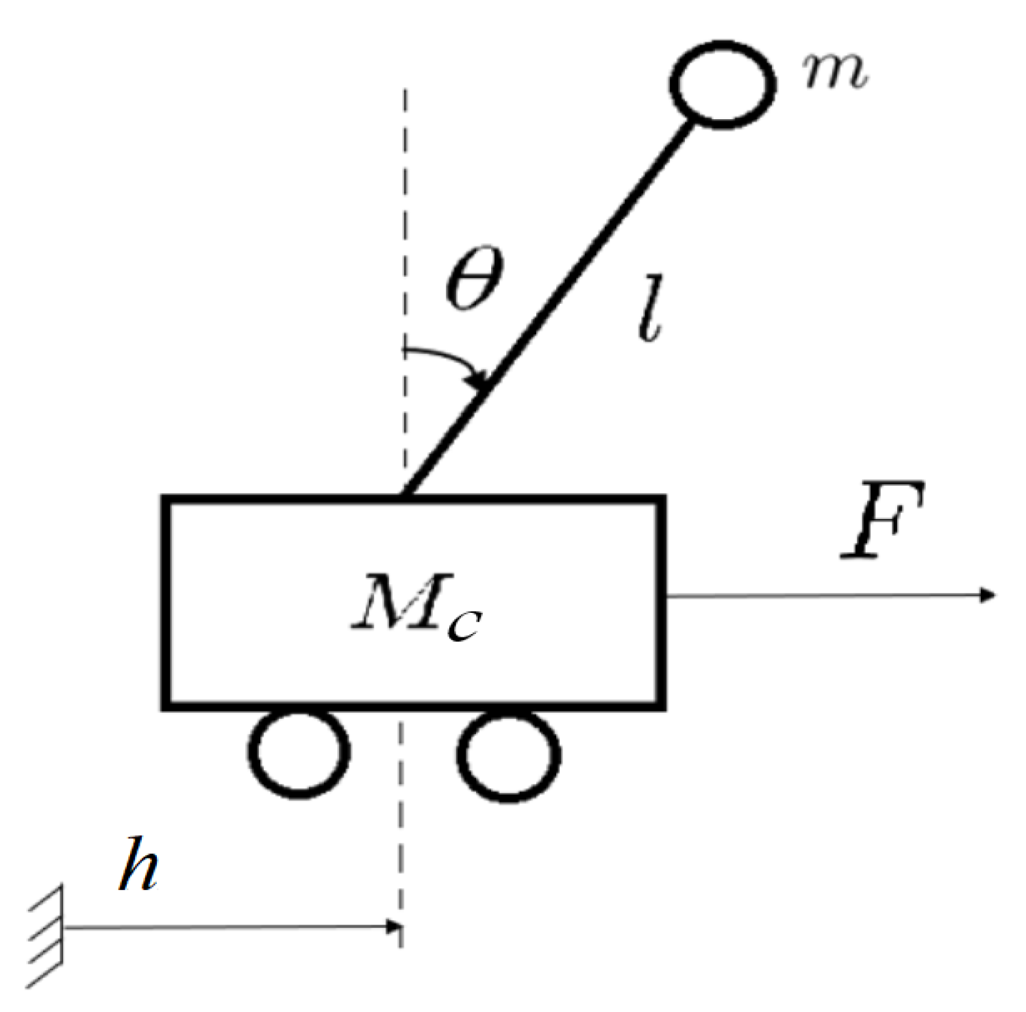
Figure 1.
Diagram of the cart inverted pendulum.
Figure 1.
Diagram of the cart inverted pendulum.
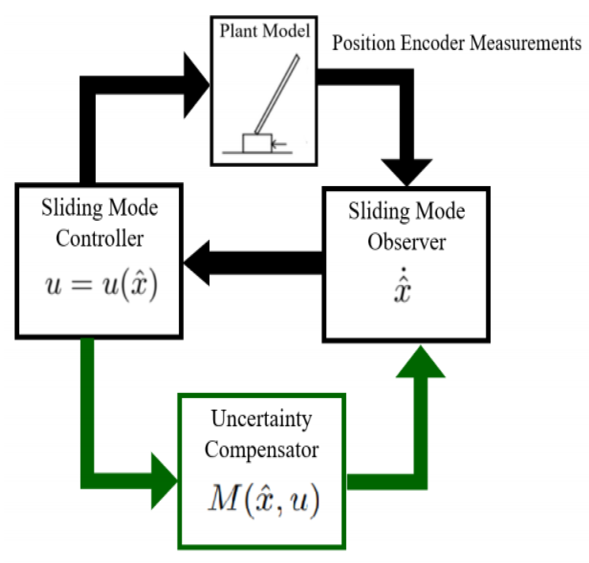
Figure 2.
High level schematic overview of the proposed sliding mode observer and controller system.
Figure 2.
High level schematic overview of the proposed sliding mode observer and controller system.
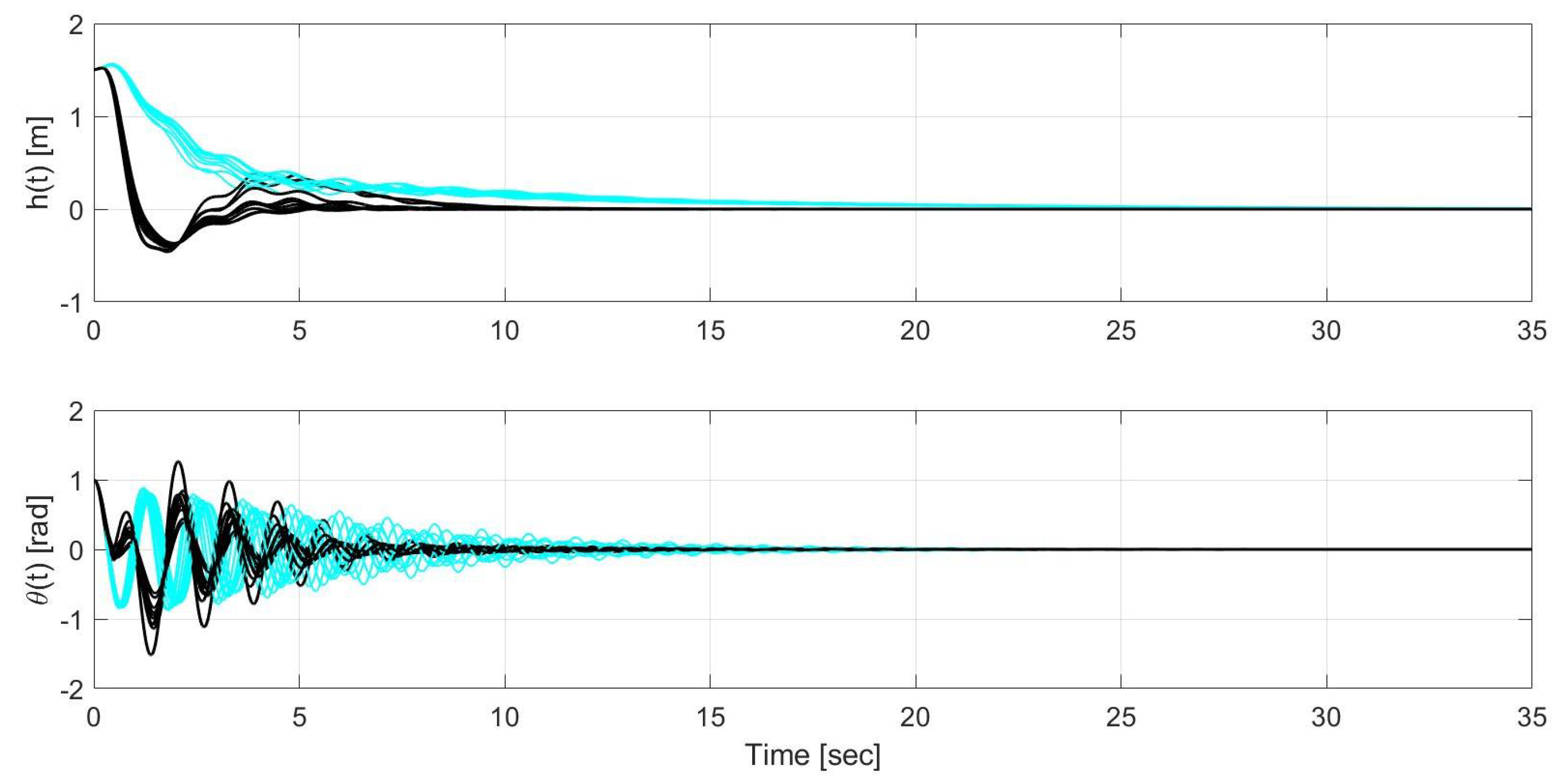
Figure 3.
Time evolution of the state and for linear quadratic regulator (LQR) without uncertainty compensation (cyan) and LQR with uncertainty compensation (black) during closed-loop operation.
Figure 3.
Time evolution of the state and for linear quadratic regulator (LQR) without uncertainty compensation (cyan) and LQR with uncertainty compensation (black) during closed-loop operation.
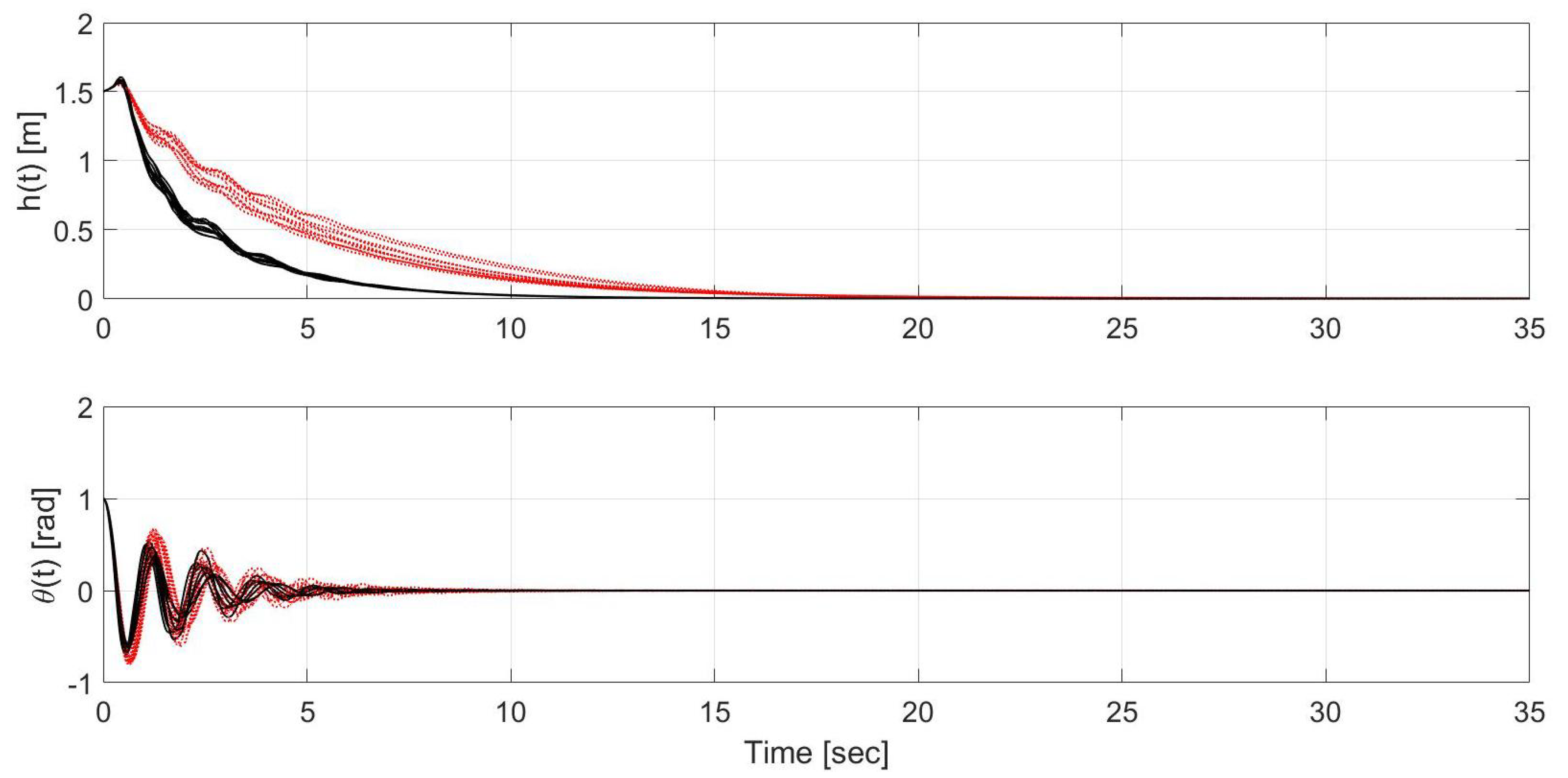
Figure 4.
Time evolution of the state and for sliding mode control (SMC) without uncertainty compensation (red) and SMC with uncertainty compensation (black) during closed-loop operation.
Figure 4.
Time evolution of the state and for sliding mode control (SMC) without uncertainty compensation (red) and SMC with uncertainty compensation (black) during closed-loop operation.
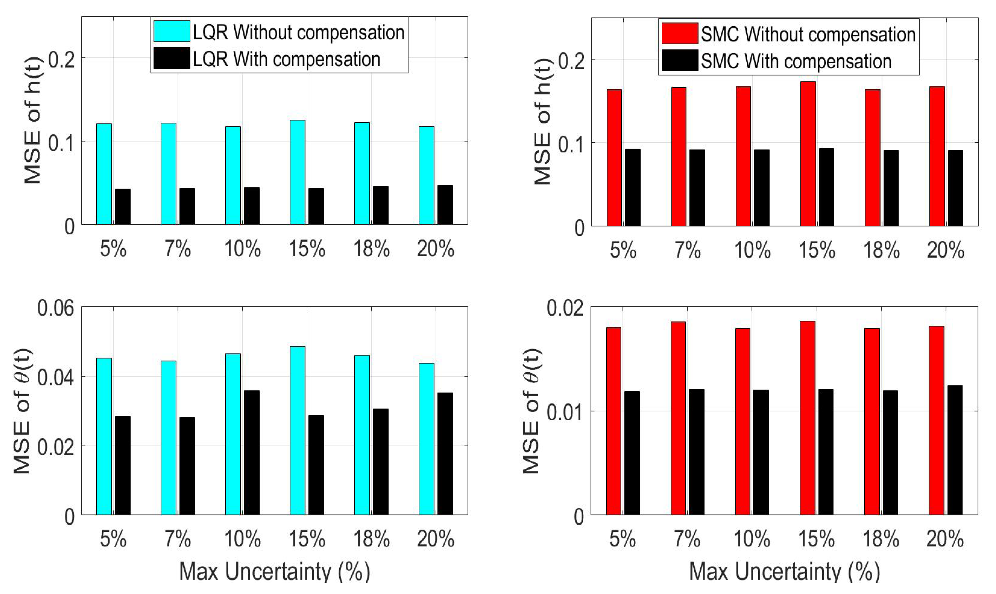
Figure 5.
Average mean squared error (MSE) during closed-loop operation for 10 iterations of randomized parameter uncertainty using LQR (left) and SMC (right) with and without uncertainty compensation.
Figure 5.
Average mean squared error (MSE) during closed-loop operation for 10 iterations of randomized parameter uncertainty using LQR (left) and SMC (right) with and without uncertainty compensation.
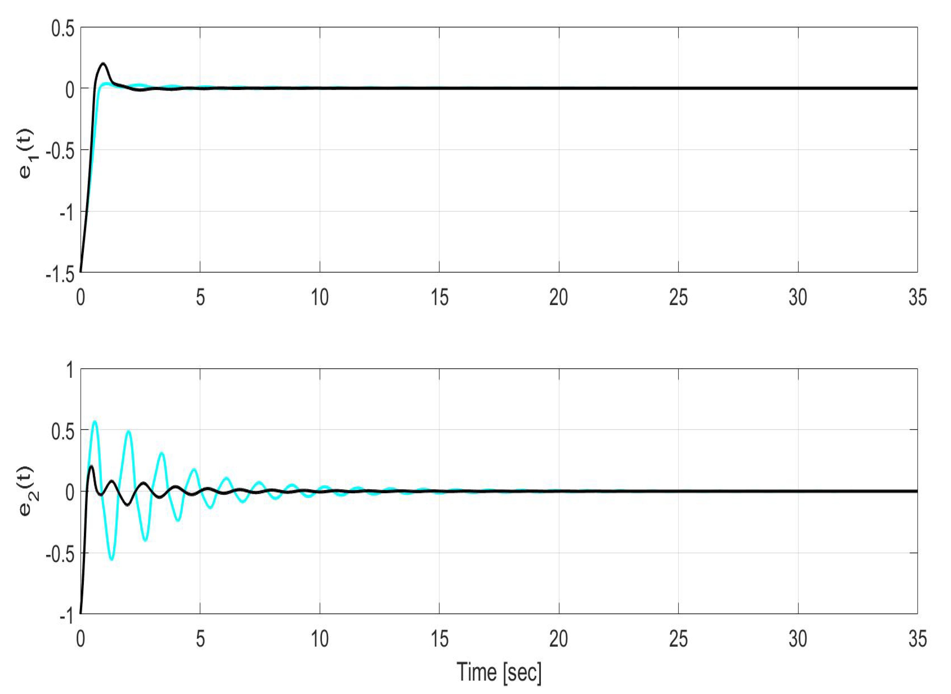
Figure 6.
Time evolution of the estimation error in states (top) and (bottom) for LQR without uncertainty compensation (cyan) and LQR with uncertainty compensation (black) over the entire simulation time.
Figure 6.
Time evolution of the estimation error in states (top) and (bottom) for LQR without uncertainty compensation (cyan) and LQR with uncertainty compensation (black) over the entire simulation time.
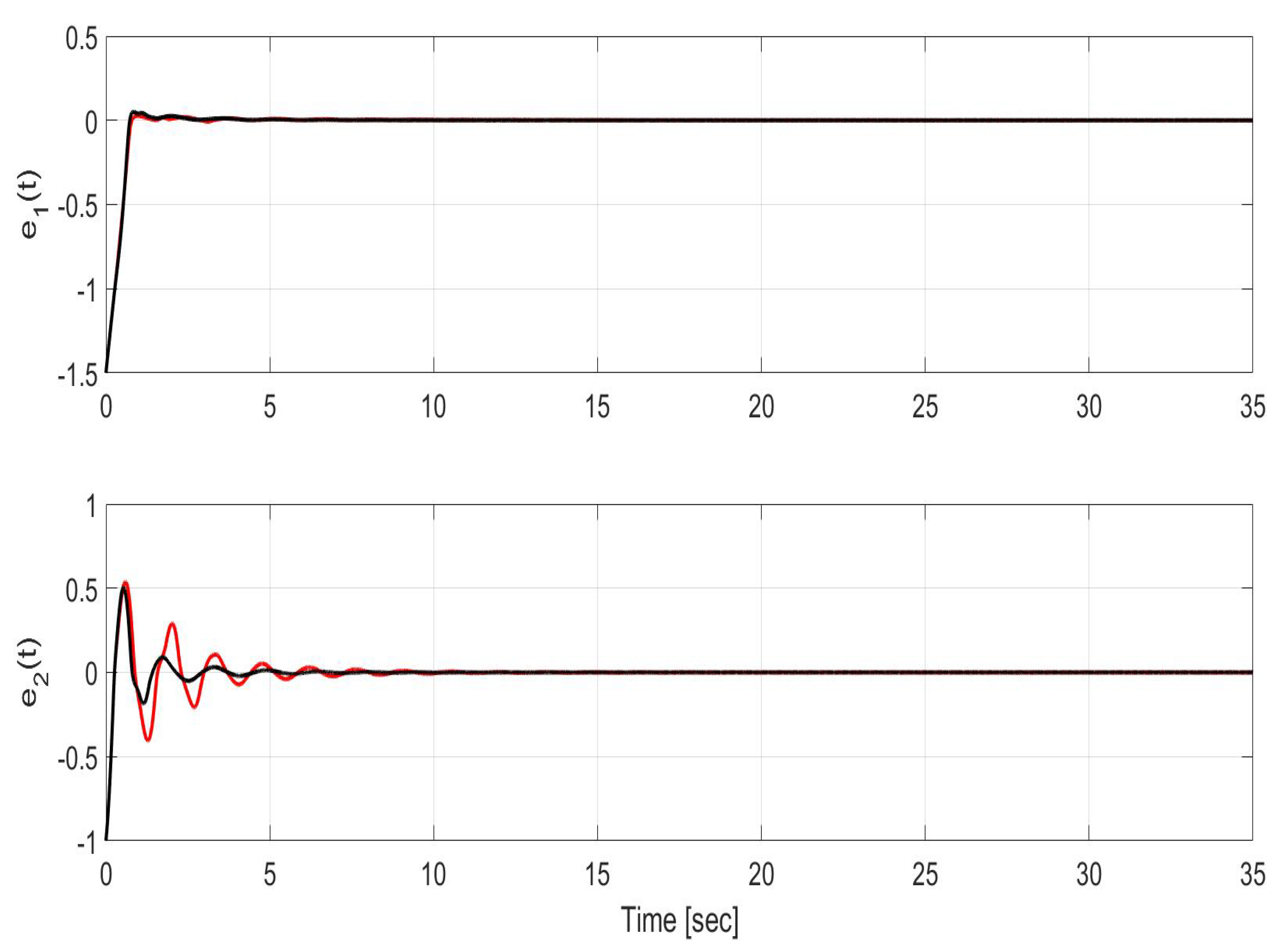
Figure 7.
Time evolution of the estimation error in states (top) and (bottom) for SMC without uncertainty compensation (red) and SMC with uncertainty compensation (black) over the entire simulation time.
Figure 7.
Time evolution of the estimation error in states (top) and (bottom) for SMC without uncertainty compensation (red) and SMC with uncertainty compensation (black) over the entire simulation time.
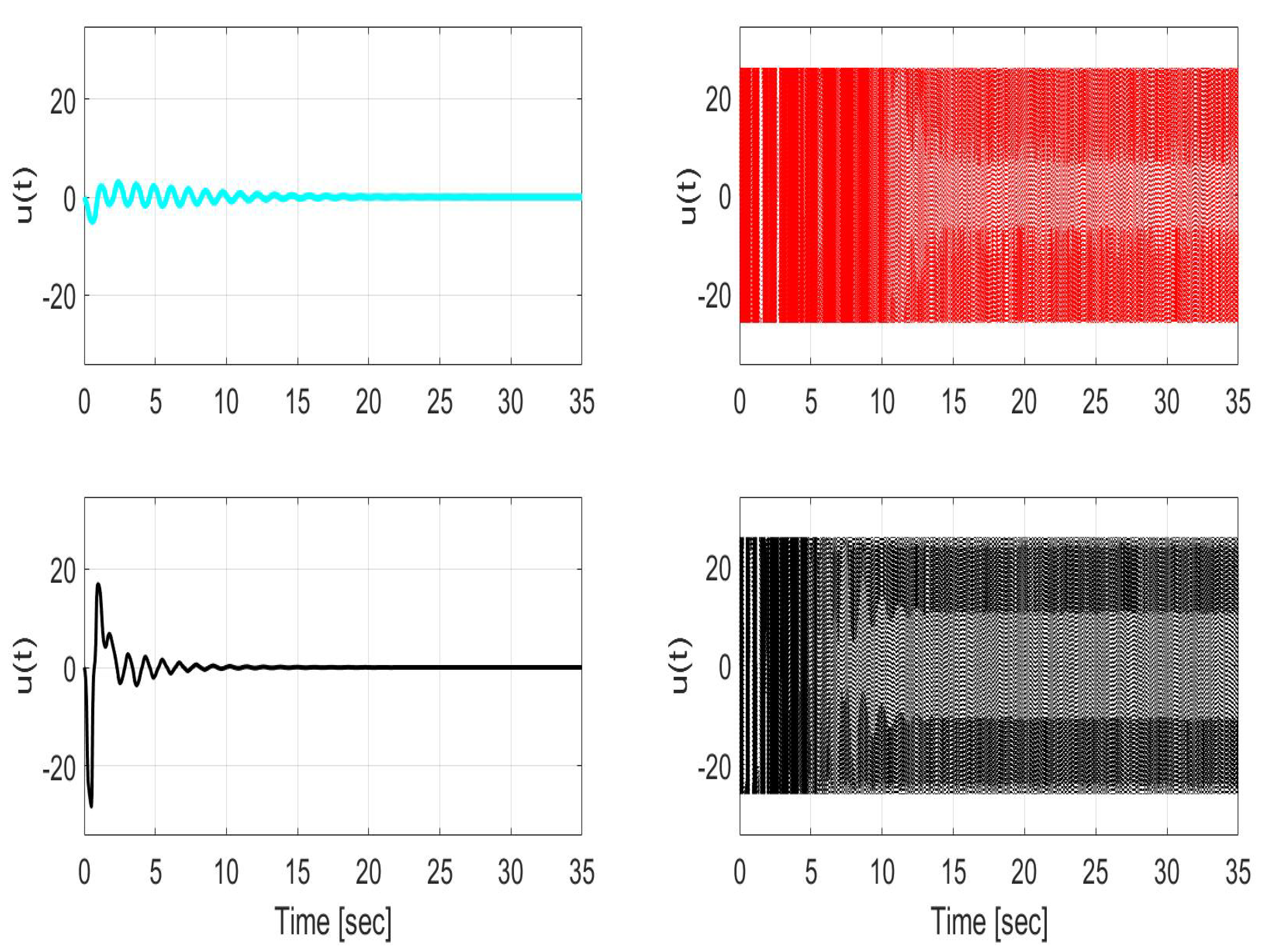
Figure 8.
Control input used for LQR (left) and SMC (right) during closed-loop operation without (top) and with (bottom) uncertainty compensation. Note that the reduction of chattering is not the focus of the current result.
Figure 8.
Control input used for LQR (left) and SMC (right) during closed-loop operation without (top) and with (bottom) uncertainty compensation. Note that the reduction of chattering is not the focus of the current result.
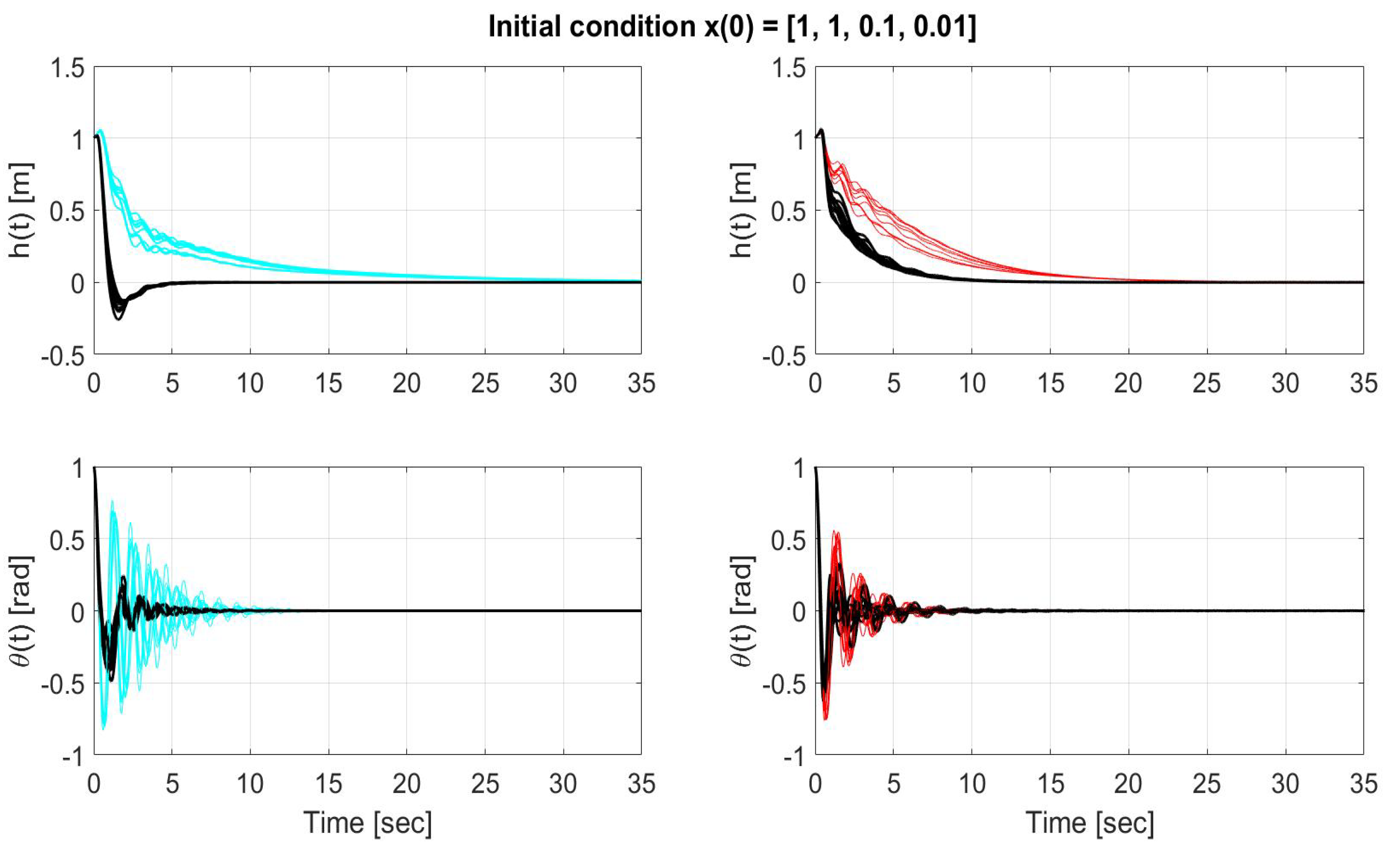
Figure 9.
Time evolution of the states (top) and (bottom) for LQR without uncertainty compensation (left-cyan), LQR with uncertainty compensation (left-black), SMC without uncertainty compensation (right-red), SMC with uncertainty compensation (right-black) over the entire simulation time for initial condition x(0) = [1, 1, 0.1, 0.01 ].
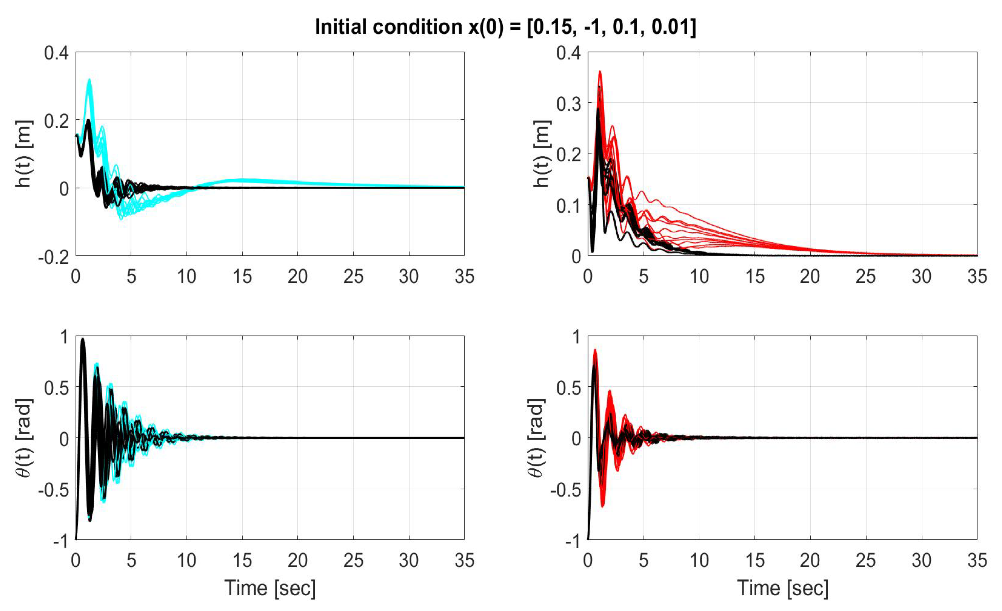
Figure 10.
Time evolution of the states (top) and (bottom) for LQR without uncertainty compensation (left-cyan), LQR with uncertainty compensation (left-black), SMC without uncertainty compensation (right-red), SMC with uncertainty compensation (right-black) over the entire simulation time for initial condition x(0) = [0.15, −1, 0.1, 0.01 ].
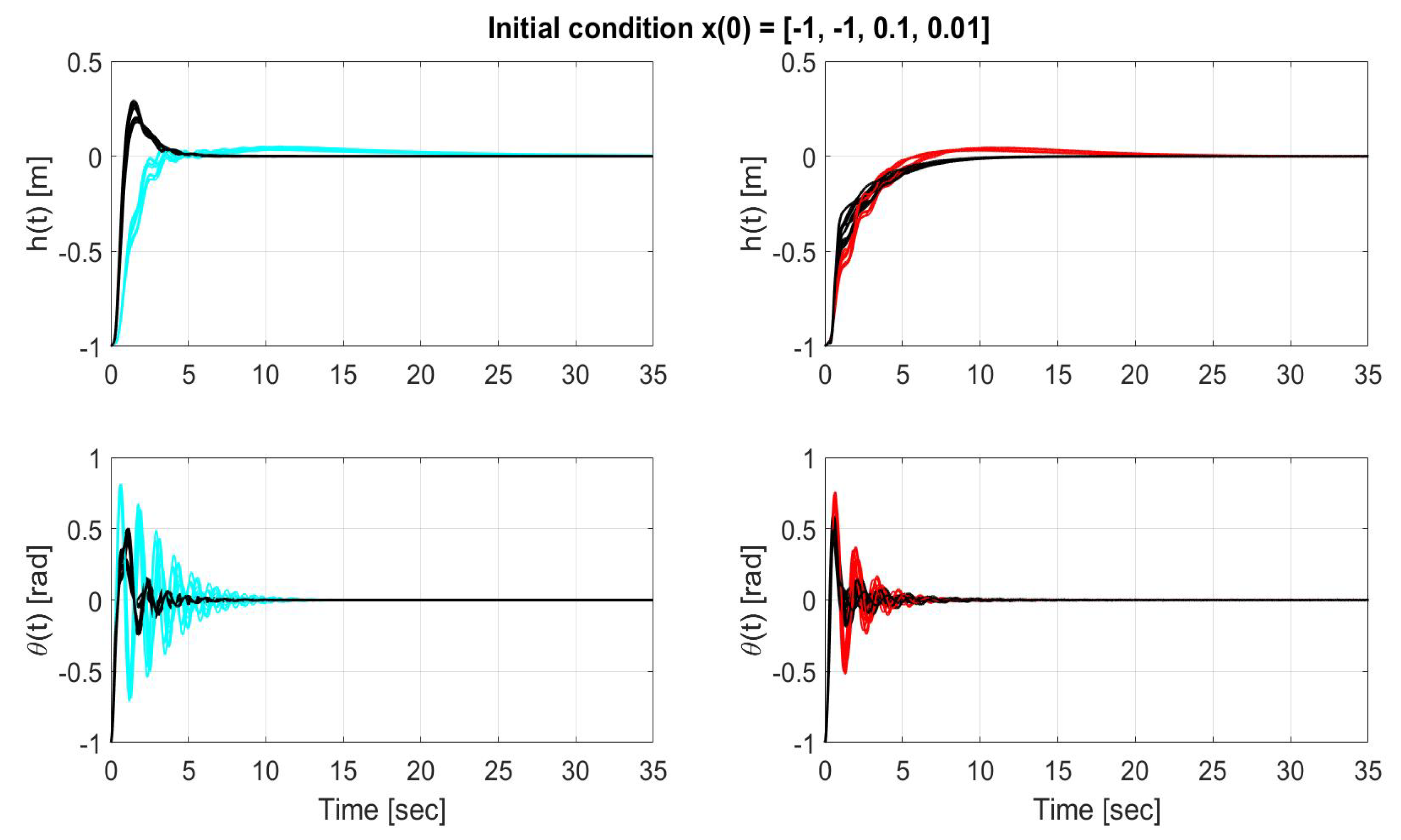
Figure 11.
Time evolution of the states (top) and (bottom) for LQR without uncertainty compensation (left-cyan), LQR with uncertainty compensation (left-black), SMC without uncertainty compensation (right-red), SMC with uncertainty compensation (right-black) over the entire simulation time for initial condition x(0) = [−1, −1, 0.1, 0.01 ].
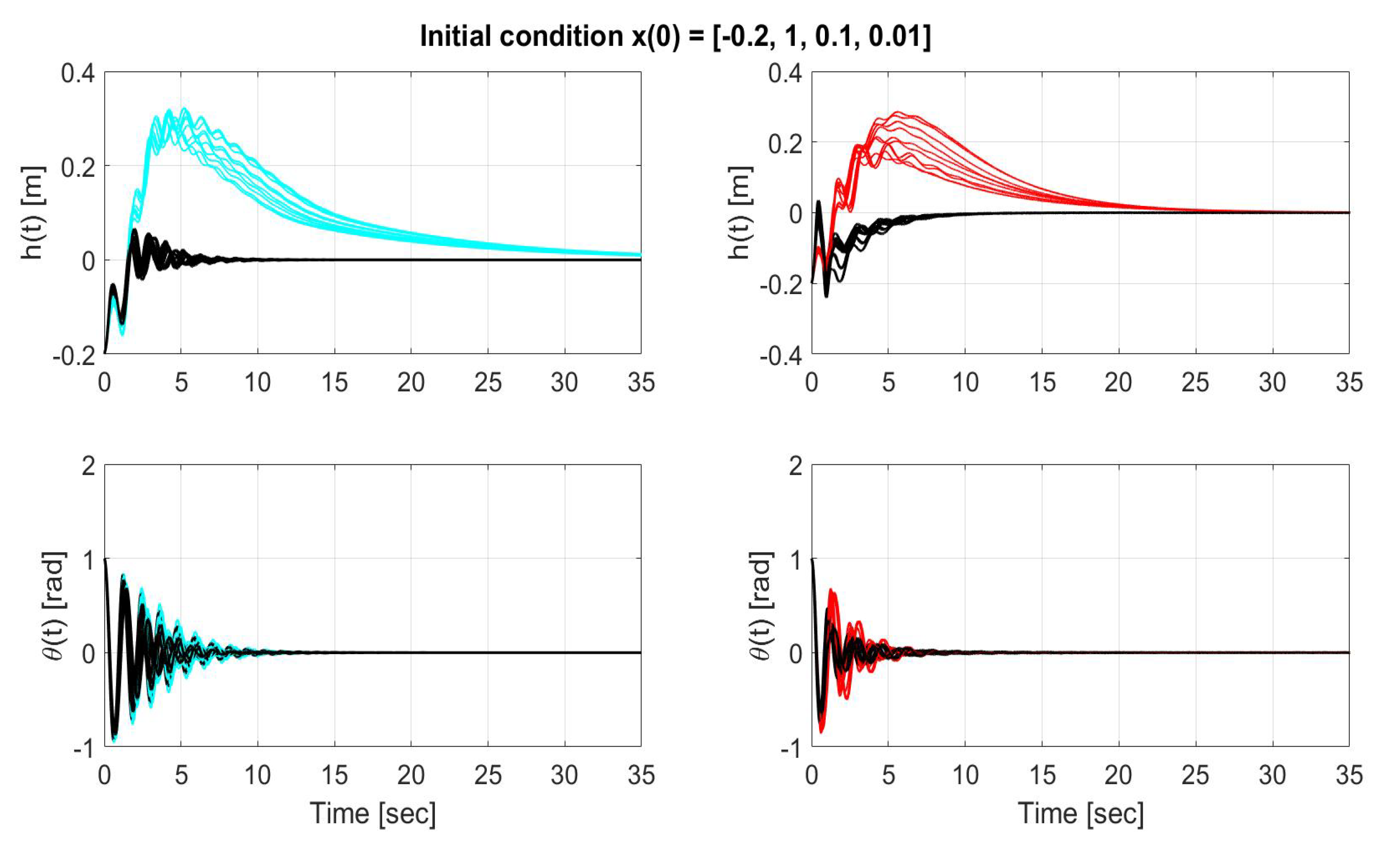
Figure 12.
Time evolution of the states (top) and (bottom) for LQR without uncertainty compensation (left-cyan), LQR with uncertainty compensation (left-black), SMC without uncertainty compensation (right-red), SMC with uncertainty compensation (right-black) over the entire simulation time for initial condition x(0) = [−0.2, 1, 0.1, 0.01 ].
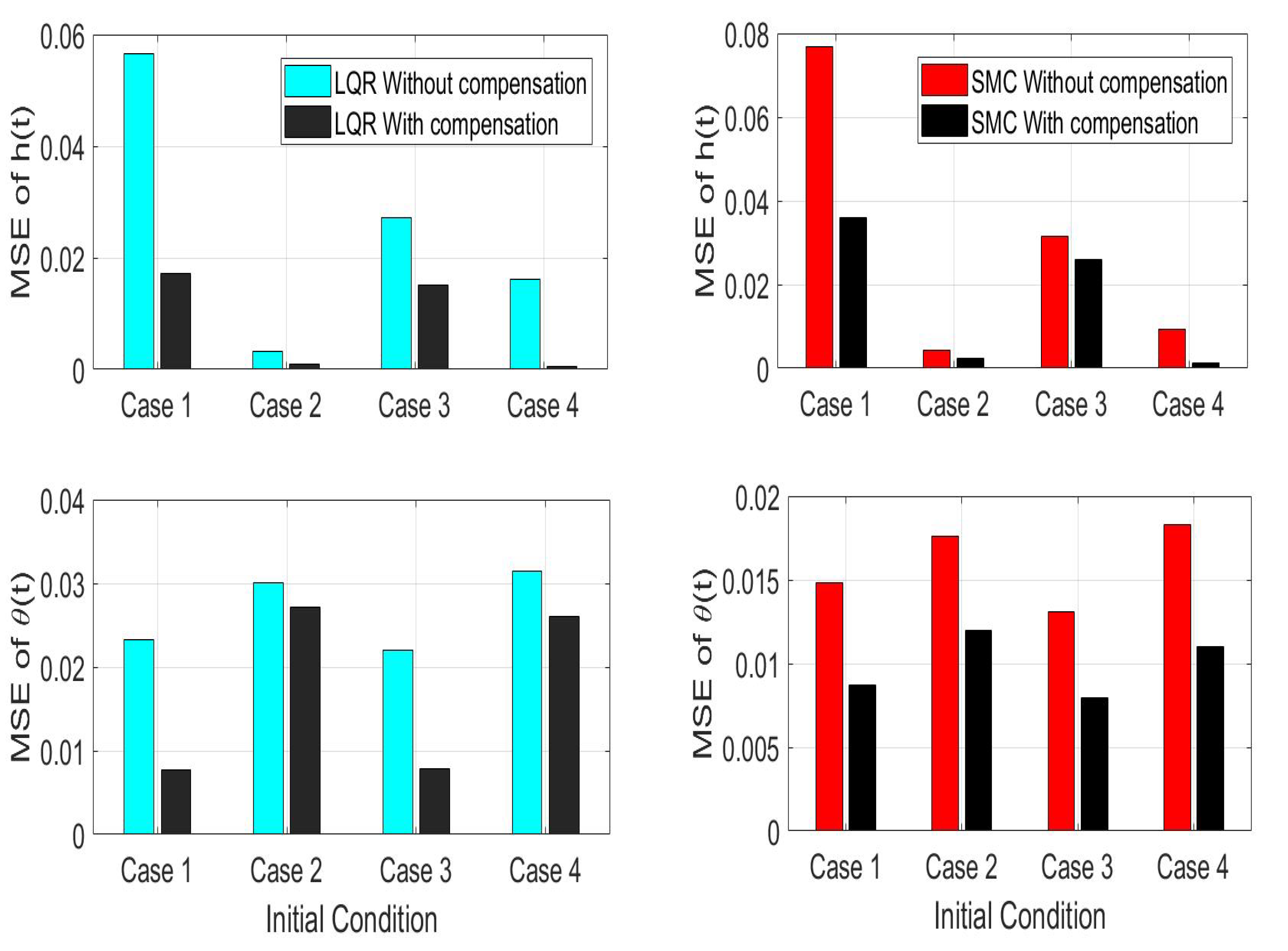
Figure 13.
Mean squared error (MSE) during closed-loop operation for 10 iterations of 4 cases of initial conditions using LQR (left) and SMC (right) with and without uncertainty compensation.
Figure 13.
Mean squared error (MSE) during closed-loop operation for 10 iterations of 4 cases of initial conditions using LQR (left) and SMC (right) with and without uncertainty compensation.
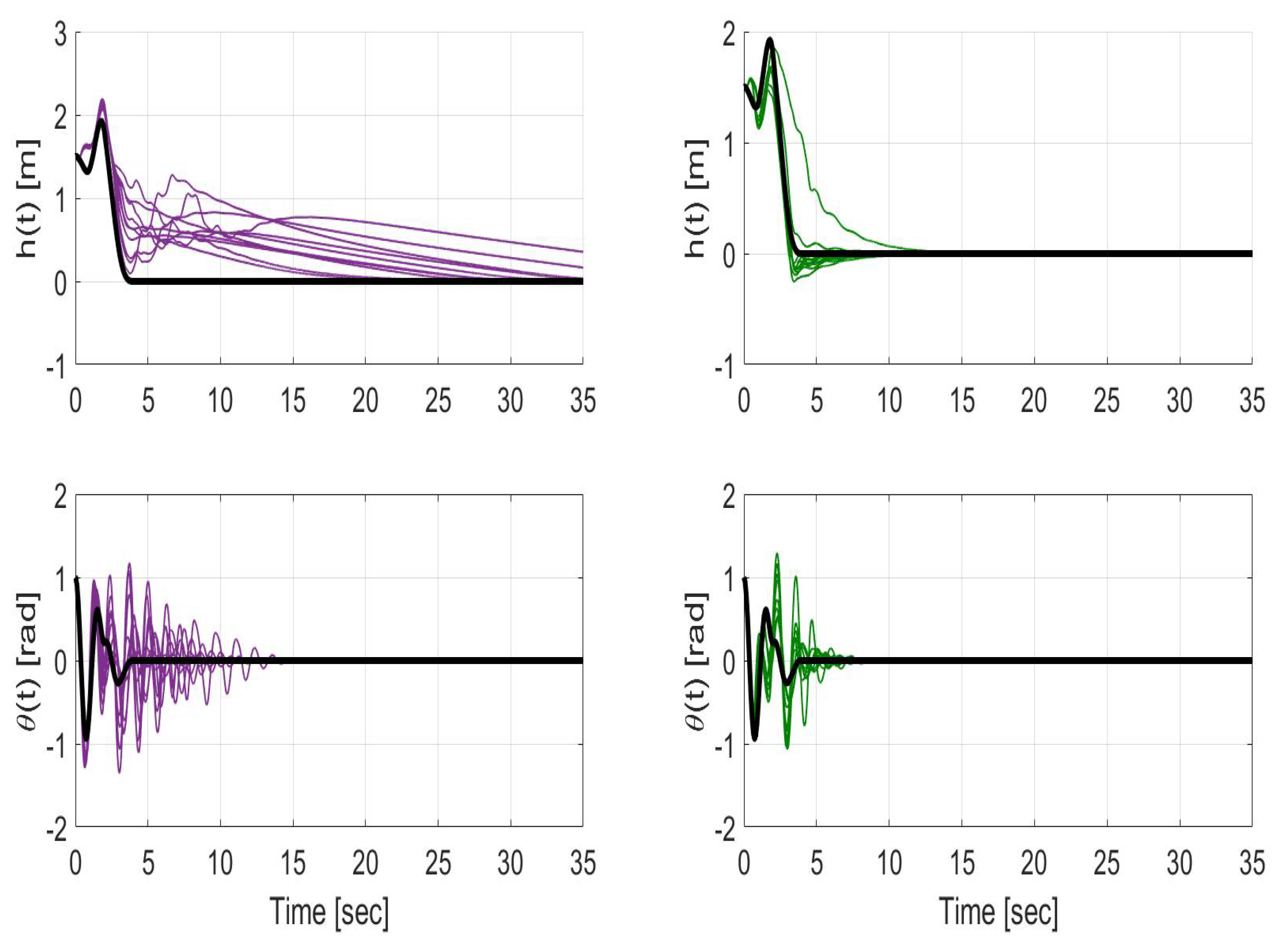
Figure 14.
Time evolution of the optimal trajectory (black solid line) and the states and during closed-loop sliding mode controller operation for the cases without uncertainty compensation (left-purple) and with uncertainty compensation (right-green) in the observer design.
Figure 14.
Time evolution of the optimal trajectory (black solid line) and the states and during closed-loop sliding mode controller operation for the cases without uncertainty compensation (left-purple) and with uncertainty compensation (right-green) in the observer design.
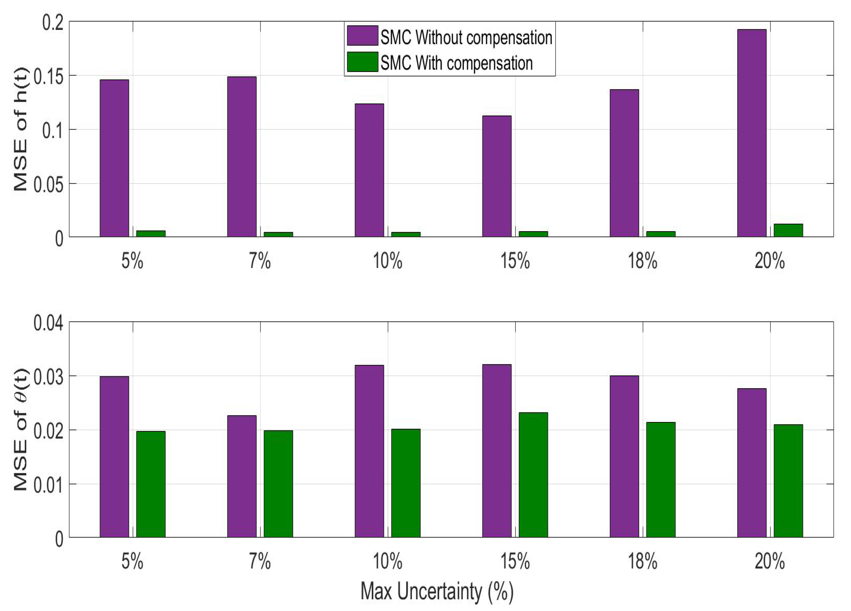
Figure 15.
Average mean squared error (MSE) during closed-loop operation over 10 iterations of randomized parameter uncertainty using the sliding mode controller with and without uncertainty compensation.
Figure 15.
Average mean squared error (MSE) during closed-loop operation over 10 iterations of randomized parameter uncertainty using the sliding mode controller with and without uncertainty compensation.
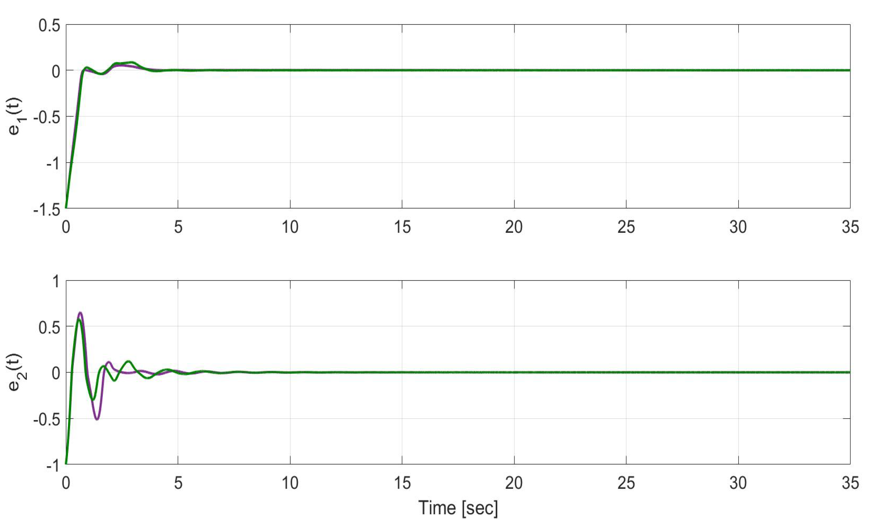
Figure 16.
Time evolution of the estimation error in states (top) and (bottom) for SMC optimal trajectory tracking without uncertainty compensation (purple) and SMC optimal trajectory tracking with uncertainty compensation (green).
Figure 16.
Time evolution of the estimation error in states (top) and (bottom) for SMC optimal trajectory tracking without uncertainty compensation (purple) and SMC optimal trajectory tracking with uncertainty compensation (green).
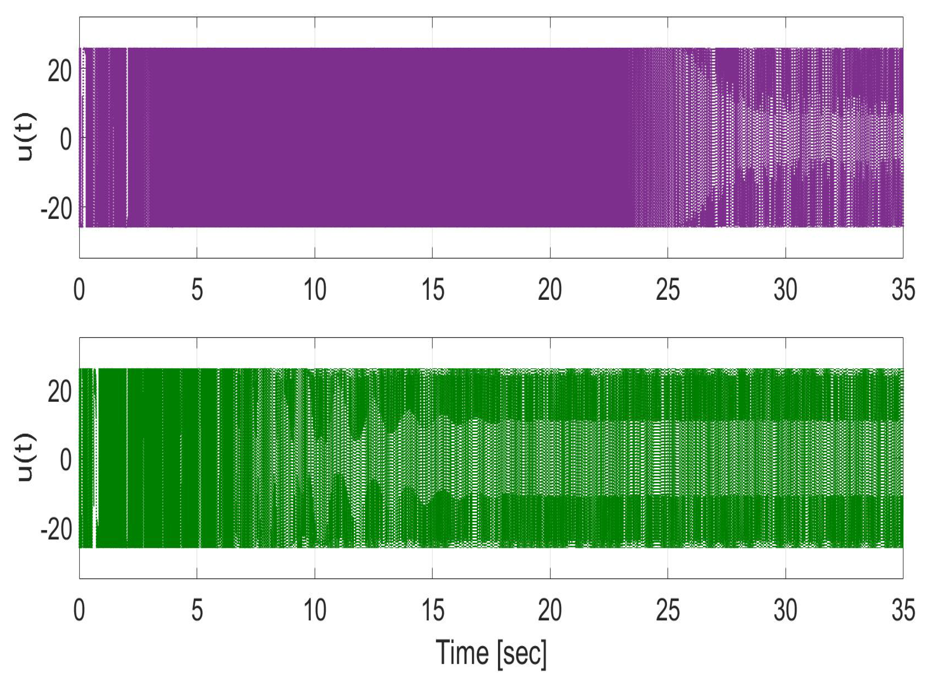
Figure 17.
Control input used for SMC during closed-loop trajectory tracking control operation without (top) and with (bottom) uncertainty compensation. Note that the reduction of chattering is not the focus of the current result.
Figure 17.
Control input used for SMC during closed-loop trajectory tracking control operation without (top) and with (bottom) uncertainty compensation. Note that the reduction of chattering is not the focus of the current result.
Table 1.
Software details.
Table 1.
Software details.
| Software | Version | Settings |
|---|
| MATLAB/Simulink | R2017b | Simulation/Model configuration Parameters / Solver Options |
| Type : Fixed step |
| Solver : ode4 (Runge-Kutta) |
| Fixed step size : 0.001 |
Table 2.
Nominal parameter values.
Table 2.
Nominal parameter values.
| = kg |
| m = kg |
| l = m |
| g = −9.8 m/s2 |
Table 3.
Observer gains.
| | |
|---|
| 2 | 2 |
| 2 | 2 |
| | |
| | |
| | |
| | |
Table 4.
Mean squared error (MSE) and root mean squared error (RMS) during closed-loop operation for 10 iterations of randomized parameter uncertainty using LQR and SMC (Regulation) with uncertainty compensation (With C) and without uncertainty compensation (W/o C).
Table 4.
Mean squared error (MSE) and root mean squared error (RMS) during closed-loop operation for 10 iterations of randomized parameter uncertainty using LQR and SMC (Regulation) with uncertainty compensation (With C) and without uncertainty compensation (W/o C).
| LQR REGULATION |
|---|
| Unc | MSE of | MSE of | RMS of | RMS of |
| (%) | W/o C | With C | W/o C | With C | W/o C | With C | W/o C | With C |
| 5 | 0.1214 | 0.0432 | 0.04516 | 0.02842 | 0.3484 | 0.2078 | 0.2125 | 0.1686 |
| 7 | 0.1216 | 0.0436 | 0.04435 | 0.02798 | 0.3487 | 0.2088 | 0.2106 | 0.1673 |
| 10 | 0.1175 | 0.04448 | 0.04632 | 0.03572 | 0.3428 | 0.2109 | 0.2152 | 0.1890 |
| 15 | 0.125 | 0.04392 | 0.04838 | 0.02856 | 0.3536 | 0.2096 | 0.2200 | 0.1690 |
| 18 | 0.1227 | 0.04655 | 0.04595 | 0.0306 | 0.3503 | 0.2158 | 0.2144 | 0.1749 |
| 20 | 0.1178 | 0.04754 | 0.04362 | 0.03506 | 0.3432 | 0.2180 | 0.2089 | 0.1872 |
| Average | 0.121 | 0.044882 | 0.04563 | 0.031057 | 0.34783 | 0.21182 | 0.213582 | 0.176003 |
| Reduction (%) | 62.91 | 31.94 | 39.10 | 17.59 |
| SMC REGULATION |
| Unc | MSE of | MSE of | RMS of | RMS of |
| (%) | W/o C | With C | W/o C | With C | W/o C | With C | W/o C | With C |
| 5 | 0.164 | 0.09204 | 0.01795 | 0.01181 | 0.4050 | 0.3034 | 0.1340 | 0.1087 |
| 7 | 0.1658 | 0.09162 | 0.01849 | 0.01202 | 0.4072 | 0.3027 | 0.1360 | 0.1096 |
| 10 | 0.167 | 0.09136 | 0.01789 | 0.01201 | 0.4087 | 0.3023 | 0.1338 | 0.1096 |
| 15 | 0.1735 | 0.09301 | 0.01861 | 0.01208 | 0.4165 | 0.3050 | 0.1364 | 0.1099 |
| 18 | 0.164 | 0.09045 | 0.01791 | 0.01192 | 0.4050 | 0.3007 | 0.1338 | 0.1092 |
| 20 | 0.167 | 0.09048 | 0.0181 | 0.01243 | 0.4087 | 0.3008 | 0.1345 | 0.1115 |
| Average | 0.166883 | 0.091493 | 0.018158 | 0.012045 | 0.408495 | 0.302475 | 0.134749 | 0.109746 |
| Reduction (%) | 45.18 | 33.67 | 25.95 | 18.55 |
Table 5.
Mean squared error (MSE) during closed-loop operation for 10 iterations of randomized parameter uncertainty using LQR and SMC (Regulation) with uncertainty compensation (With C) and without uncertainty compensation (W/o C) for 4 different cases of initial conditions.
Table 5.
Mean squared error (MSE) during closed-loop operation for 10 iterations of randomized parameter uncertainty using LQR and SMC (Regulation) with uncertainty compensation (With C) and without uncertainty compensation (W/o C) for 4 different cases of initial conditions.
| LQR REGULATION |
|---|
| Initial Conditions | MSE of | MSE of |
| W/o C | With C | Reduction % | W/o C | With C | Reduction % |
| Case 1 x(0) = [1, 1, 0.1, 0.01 ] | 0.05649 | 0.01711 | 69.71 | 0.02331 | 0.007758 | 66.72 |
| Case 2 x(0) = [0.15, −1, 0.1, 0.01 ] | 0.00316 | 0.001015 | 67.88 | 0.03001 | 0.02714 | 9.56 |
| Case 3 x(0) = [−1, −1, 0.1, 0.01 ] | 0.02721 | 0.01519 | 44.17 | 0.02195 | 0.007832 | 64.32 |
| Case 4 x(0) = [−0.2, 1, 0.1, 0.01 ] | 0.01622 | 0.0006201 | 96.18 | 0.03143 | 0.02609 | 16.99 |
| Average | 0.02577 | 0.0084838 | 69.49 | 0.026675 | 0.017205 | 39.40 |
| SMC REGULATION |
| Initial Conditions | MSE of | MSE of |
| W/o C | With C | Reduction % | W/o C | With C | Reduction % |
| Case 1 x(0) = [1, 1, 0.1, 0.01 ] | 0.07693 | 0.03594 | 53.28 | 0.01481 | 0.008727 | 41.07 |
| Case 2 x(0) = [0.15, −1, 0.1, 0.01 ] | 0.004334 | 0.002419 | 44.19 | 0.0176 | 0.01196 | 32.05 |
| Case 3 x(0) = [−1, −1, 0.1, 0.01 ] | 0.03142 | 0.02597 | 17.35 | 0.01307 | 0.00794 | 39.25 |
| Case 4 x(0) = [−0.2, 1, 0.1, 0.01 ] | 0.009186 | 0.001317 | 85.66 | 0.01832 | 0.01099 | 40.01 |
| Average | 0.030468 | 0.0164115 | 50.12 | 0.01595 | 0.009904 | 38.10 |
Table 6.
Control gains.
| k1 = 2 | Z0 = 26 |
| k2 = 5 | λ = 30 |
| k3 = 5 | ε = 0.1460 |
| k4 = 1 | |
Table 7.
Mean squared error (MSE) during closed-loop operation for 10 iterations of randomized parameter uncertainty using SMC (Tracking) with uncertainty compensation (With C) and without uncertainty compensation (W/o C).
Table 7.
Mean squared error (MSE) during closed-loop operation for 10 iterations of randomized parameter uncertainty using SMC (Tracking) with uncertainty compensation (With C) and without uncertainty compensation (W/o C).
| SMC TRACKING |
|---|
| Uncertainty | MSE of | MSE of | RMS of | RMS of |
| (%) | W/o C | With C | W/o C | With C | W/o C | With C | W/o C | With C |
| 5 | 0.1453 | 0.005788 | 0.02985 | 0.01963 | 0.3812 | 0.0761 | 0.1728 | 0.1401 |
| 7 | 0.1485 | 0.004584 | 0.02251 | 0.01976 | 0.3854 | 0.0677 | 0.1500 | 0.1406 |
| 10 | 0.1233 | 0.004682 | 0.03194 | 0.02003 | 0.3511 | 0.0684 | 0.1787 | 0.1415 |
| 15 | 0.1118 | 0.005419 | 0.03198 | 0.02311 | 0.3344 | 0.0736 | 0.1788 | 0.1520 |
| 18 | 0.1367 | 0.005004 | 0.02999 | 0.02135 | 0.3697 | 0.0707 | 0.1732 | 0.1461 |
| 20 | 0.192 | 0.01245 | 0.02757 | 0.02089 | 0.4382 | 0.1116 | 0.1660 | 0.1445 |
| Average | 0.142933 | 0.006321 | 0.028973 | 0.020795 | 0.376659 | 0.078024 | 0.169928 | 0.144146 |
| Reduction (%) | 95.58 | 28.23 | 79.29 | 15.17 |


