
A Method of Optimizing Terrain Rendering Using Digital Terrain Analysis

1
College of Geodesy and Geomatics, Shandong University of Science and Technology, Qingdao 266590, China
2
Key Laboratory of Marine Environmental Survey Technology and Application, Ministry of Natural Resources, Guangzhou 510000, China
3
South China Sea Information Center of State Oceanic Administration, Guangzhou 510000, China
4
North Sea Engineering and Survey and Research Institute, State Oceanic Administration, Qingdao 266061, China
5
Qingdao Yuehai Information Service Co., Ltd., Qingdao 266590, China
*
Author to whom correspondence should be addressed.
ISPRS Int. J. Geo-Inf. 2021, 10(10), 666; https://0-doi-org.brum.beds.ac.uk/10.3390/ijgi10100666
Submission received: 20 August 2021
/
Revised: 24 September 2021
/
Accepted: 27 September 2021
/
Published: 1 October 2021
Abstract
:Terrain rendering is an important issue in Geographic Information Systems and other fields. During large-scale, real-time terrain rendering, complex terrain structure and an increasing amount of data decrease the smoothness of terrain rendering. Existing rendering methods rarely use the features of terrain to optimize terrain rendering. This paper presents a method to increase rendering performance through precomputing roughness and self-occlusion information making use of GIS-based Digital Terrain Analysis. Our method is based on GPU tessellation. We use quadtrees to manage patches and take surface roughness in Digital Terrain Analysis as a factor of Levels of Detail (LOD) selection. Before rendering, we first regularly partition the terrain scene into view cells. Then, for each cell, we calculate its potential visible patch set (PVPS) using a visibility analysis algorithm. After that, A PVPS Image Pyramid is built, and each LOD level has its corresponding PVPS. The PVPS Image Pyramid is stored on a disk and is read into RAM before rendering. Based on the PVPS Image Pyramid and the viewpoint’s position, invisible terrain areas that are not culled through view frustum culling can be dynamically culled. We use Digital Elevation Model (DEM) elevation data of a square area in Henan Province to verify the effectiveness of this method. The experiments show that this method can increase the frame rate compared with other methods, especially for lower camera flight heights.
1. Introduction
Three-dimensional terrain rendering is an important subject of research in Geographic Information System (GIS). In recent years, with the increasingly higher requirements for realistic rendering, large-scale, high-precision, real-time terrain rendering methods are facing challenges.
These techniques can be divided into two categories: grid-based terrain modeling and triangulation-based terrain modeling [1]. The former method makes use of height data collected or arranged in the form of a regular (e.g., rectangular or square) grid; it has simple geometric structure and is widely used, but one of its shortcomings is that it is not related to the characteristics of the terrain itself. The latter method uses Triangulated Irregular Networks (TIN), which can reduce redundancy while preserving details of the terrain. This method has complex data structures and needs more storage space for topology information of triangles. In addition, a hybrid terrain model has been put forward and studied [2,3,4] in which the two aforementioned data structures are combined. Hybrid terrain models can visualize complex terrain features such as cliffs. However, hybrid terrain models have more complicated data structures and need additional processing tasks.
Sometimes terrain rendering, especially for large-scale terrains, cannot achieve the expected frame rate. However, many optimization techniques have been proposed in the last years. Hoppe successively proposes Progressive Meshes (PM) [5] and View-Dependent Progress Meshes (VDPM) framework [6]. VDPM can achieve a good performance. However, because all the vertex information in a terrain model is sent to GPU, this method has no advantage in saving bandwidth. Another representative and well-known method is Real-time Optimally Adapting Meshed (ROAM) [7], which is based on regular grids and uses two priority queues to drive splitting and merging operations. This method used a binary tree to manage triangles, and a triangle represents a node in the binary tree. Splitting operations can replace triangles with its two child triangles. Merging operations can merge two child triangles into one father triangle. These operations maintain continuous triangulations built from preprocessed bintree triangles.
Chunked Levels of Detail (Chunk LOD) [8] is an approach to aggregated LOD. LOD are usually computed and used when rendering a terrain, and they improve rendering performance by adjusting the number of triangles. Compared with the previous methods, Chunk LOD reduces the amount of CPU calculation. In addition to LOD, view frustum culling is also used to accelerate rendering in these methods. View frustum culling culls groups of triangles outside the viewing frustum at the CPU stage instead of discarding them by hardware automatically [9].
Though these methods have simplified data to be rendered to some extent, they have complex data structures and need large transmission bandwidths [10]. As hardware improves, some researchers start using GPU based methods [4,11,12], which greatly improve the rendering speed. After tessellation, which provide a way to tessellate geometry on the GPU [13], was added to rendering pipeline, hardware tessellation technology has become popular and widely used in terrain rendering of commercial game engines, such as Unreal 4 from Epic Games Inc. and Unity from Unity Technologies. Schäfer et al. discuss and compare methods of rendering based on hardware tessellation in their report [14]. Hardware tessellation technology uses axis-aligned quad patches as primitives. It usually utilizes a displacement map to determine the location of sample points generated in fix-function tessellator. Displacement maps store terrain height information and topological information implied. This method reduces primitives sending from CPU to GPU. On the basis of the new graphics card that supports tessellation, many methods have been developed. Yusov et al. use vertical skirts to hide cracks [15]. Engel et al. [16] present an algorithm that achieves smooth LODs transitions from any viewpoint. Cantlay [17] introduces his crack-free terrain, but his work ignores the terrain roughness. Some methods [18,19,20,21] use quadtrees to manage data and adopt view frustum culling to minimize data passed to GPU.
Nevertheless, we notice that some methods ignore occlusion culling. A large number of invisible primitives are sent to GPU during real-time rendering. Our approach is dedicated to solving this problem to a certain extent by using potential visible patch set (PVPS) to cull an invisible area when rendering terrain. Airely et al. first used a precomputed potential visible set (PVS) to cull hidden geometries in real-time rendering [22]. PVS is used in many graphics applications to cope with large amounts of data [23,24]. Zaugg et al. introduce this idea into terrain rendering [25]. In traditional terrain rendering, which uses triangulation-based modeling, it is difficult for PVS to reject invisible primitives because its data is organized vertex-by-vertex, and it usually consists of millions of vertexes. As a result, visibility information is hard to calculate and store. However, the emergence of hardware tessellation can apply PVS easily. In this method, the terrain is divided into quad regular patches, and there is no need to pay attention to the details of each vertex; therefore, information about invisible and visible patches could be easily stored. Table 1 lists and compares parts of the methods referred to above.
Here, we propose a viewpoint-based, seamless method to avoid sending unnecessary primitives to rendering pipeline using hardware tessellation. We partition the scene into cells and calculate a PVPS for each cell. Viewpoints in the same cell share the same PVPS; therefore, it is feasible to calculate and store every viewpoint’s PVPS, even with limited storage capacity. We use quadtrees to manage patches. Patches are created based on their father node, and roughness is taken as a factor in LOD selection. For each LOD level, we calculate a PVPS image and a roughness image. We call the union of PVPS images PVPS Image Pyramid, and we call the union of roughness images Roughness Image Pyramid. We read a node’s roughness value and visibility information from Roughness Image Pyramid and PVPS Image Pyramid to decide whether a node is to split. Before nodes’ splitting, we read their visibility information from PVPS Image Pyramid. If the information shows invisible results, nodes will be discarded. We calculate a PVPS by key viewpoints’ visibility between test points on patches using a line-of-sight algorithm. Key viewpoints are a set of points that are chosen to calculate visibility information (PVPS) in a cell space. Test points are sampled on patches. Whether a patch is visible within a cell is determined by key viewpoints in this cell and test points on this patch. For each key viewpoint, we calculate the visibility with each test point. When a high enough number of visibility results turn out invisible, we consider this patch is not visible within a cell space. We use all calculation results to create a PVPS. When a viewpoint moves from one cell to its adjacent cells, we adjust primitives (patches) via PVPS. PVPS is stored as binary images on disk.
2. Methods
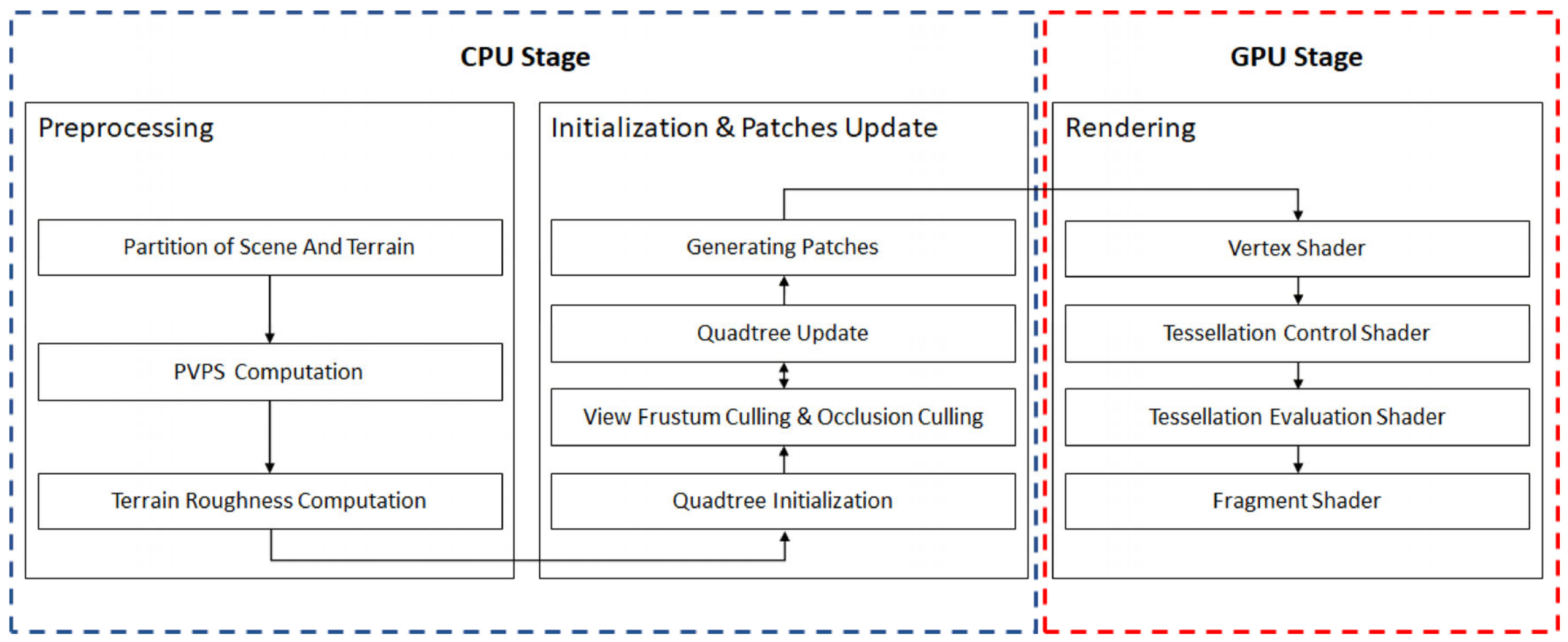
As is shown in Figure 1, our process is divided into three parts: preprocessing, initialization and patches update, and rendering.
2.1. Experimental Data
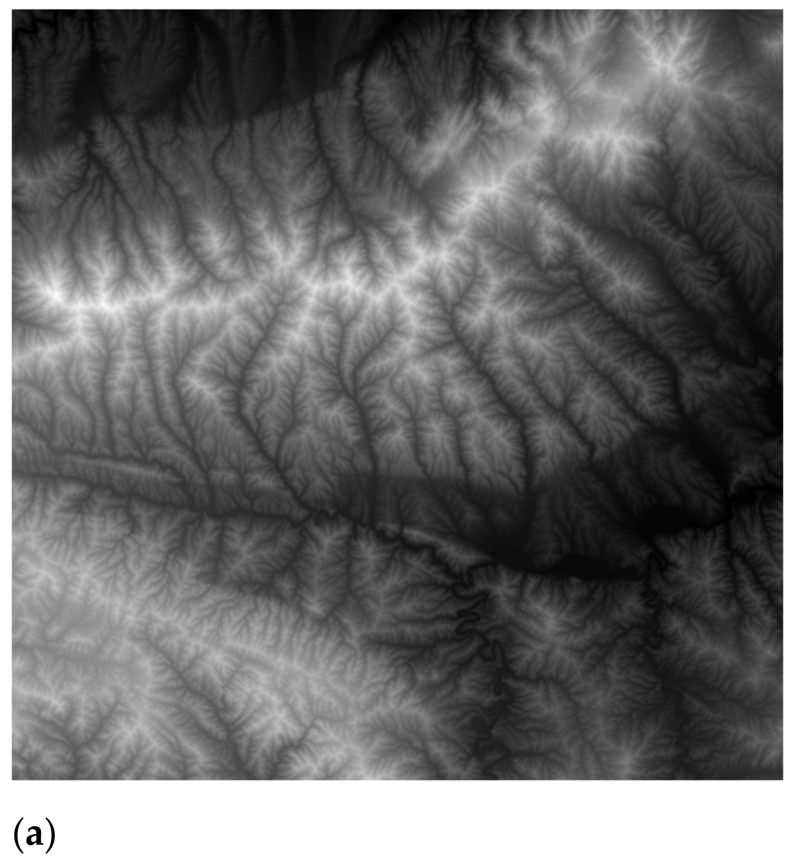
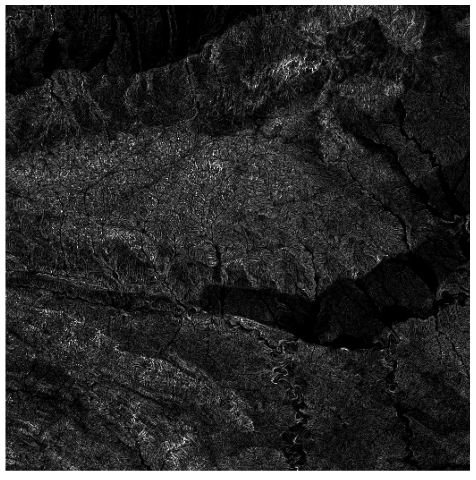
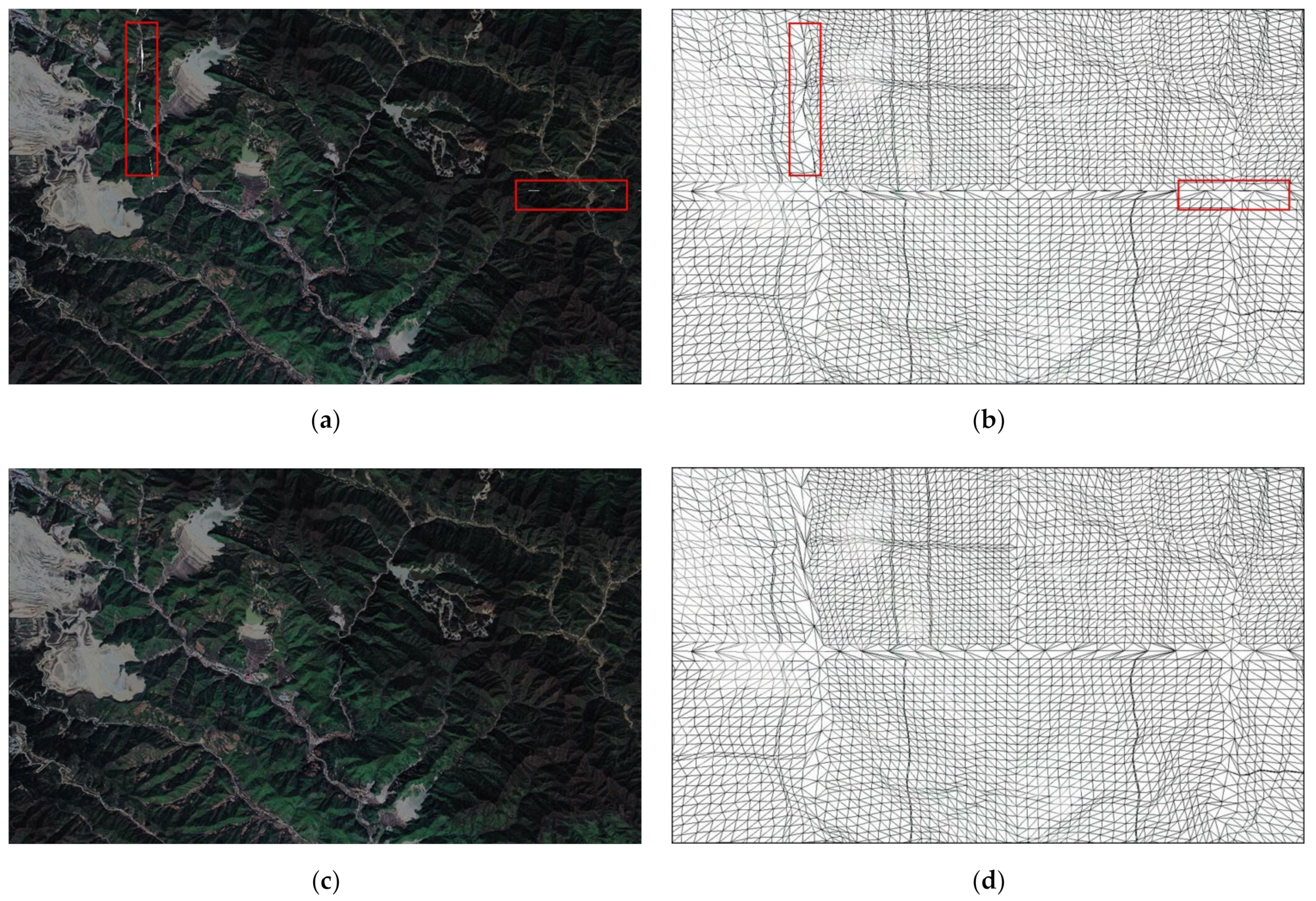
We use a 4096 × 4096 TIFF 32-bit, sampled at 12.5 m spacing, grayscale image as a height map. The data is from the southern mountainous area of Luoyang City, Henan Province, China. This area is crisscrossed with ravines and rivers. When roaming on the ground in this kind of scene, many terrain regions are occluded. Figure 2a shows this image.
2.2. Preprocessing
2.2.1. Partition of Scene and Terrain
In this section, we use a height map (texture data) to illustrate the result of terrain partition. A height map can be seen as a Digital Elevation Model (DEM), used for rendering and calculating visibility between points. A square DEM cell can be described by Equation (1).
Figure 2a shows our height map. A GPU can conveniently and efficiently perform height map texture sampling during terrain rendering.
Partitioning terrain and view scene is an important part in the whole preprocessing stage, also influencing the performance of rendering later.
The partitioning method depends on rendering quality requirements. Smaller partition intervals can result in a lot of precomputation work and taking up too much space to store PVPS information, but this can generate a precise PVPS and has a better rendering performance. A bigger partition interval can lead to a rough PVPS, relatively: more areas that should have been eliminated might be retained.
In this paper, we partition the terrain into patches. A patch represents a square terrain area and is defined by the coordinates of its four corners. The way of partition depends largely on experience. When the terrain is partitioned into more patches such as patches, we can get more triangles and, therefore, a better rendering result. As a result, more patches decrease FPS. As for the terrain of this paper, patches can meet the requirements of rendering quality. We partition the scene space into view cells. A cell represents a cuboid region in space. Cells are distributed over the surface of the terrain. There are three floors, and there are cells for each floor. The view scene not in the view cells is called . For each cell except , we calculate a PVPS. There are view cells in total. The partition process is expressed by Equations (2) and (3). Figure 2 shows the partition result.
2.2.2. PVPS Computation
This section describes the strategy we proposed to determine a cell’s Potential Visibility Patch Set (PVPS). We adopt a straightforward method based on an adapted line-of-sight algorithms to calculate visibility between one viewpoint and one test point.
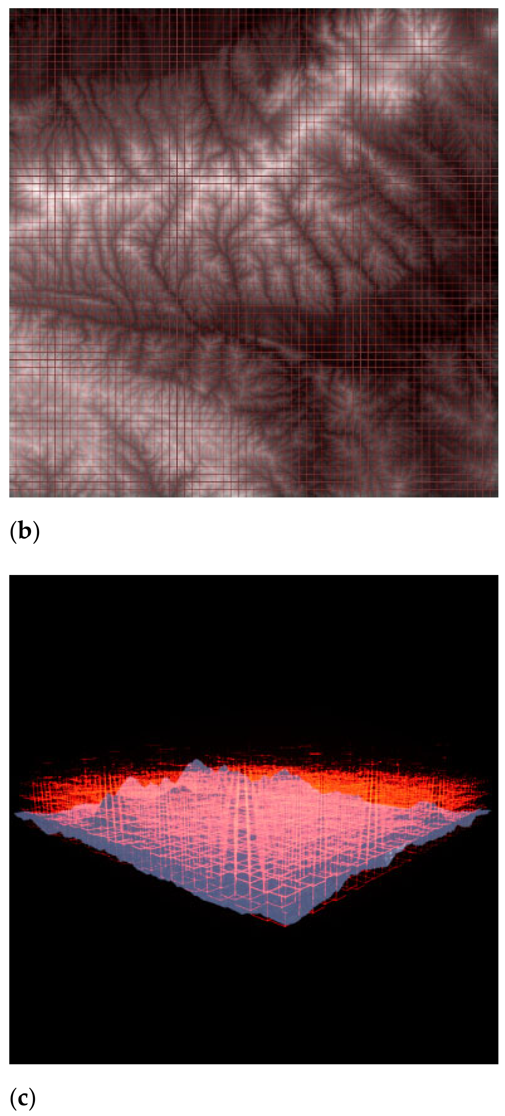
As is shown in Figure 3a, terrain section line consists of a set of points whose coordinates are obtained by a kind of 3D Bresenham algorithm [26,27]. Each point in a terrain section line is assigned the value of the nearest DEM cell.
As is shown in Figure 3b, for a point in a terrain section line, we calculate , is the vertical projection of onto the straight line connecting the view and test point. For each , we test the condition in Equation (4), where represents the angular coefficients of oriented line from to , and represents the angular coefficients of oriented line from to . If all results are less than 0, there is no visibility between the viewpoint and the test point; otherwise, they are intervisible.
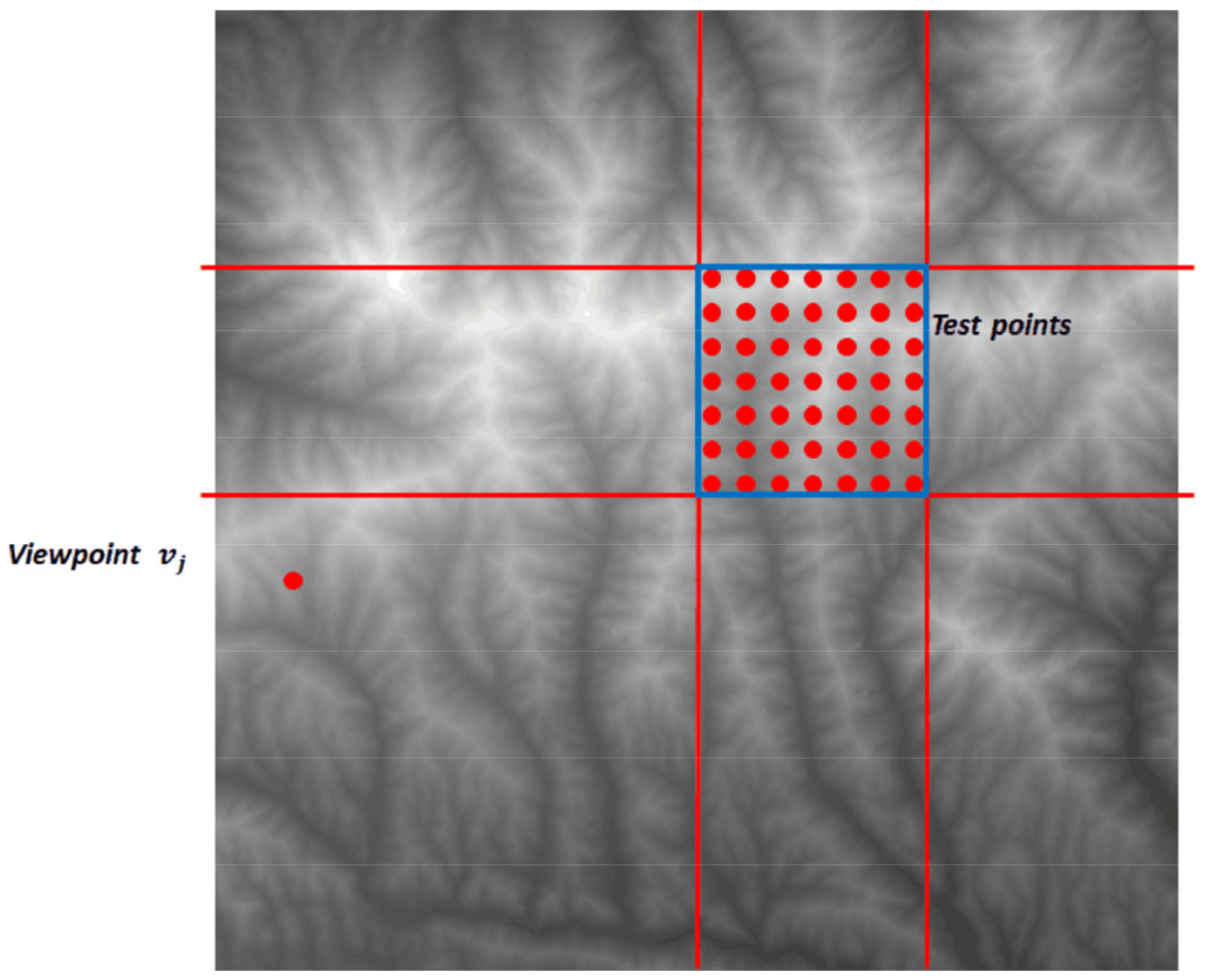
Test points are evenly distributed in a patch area, test points in total, as are shown in Figure 4. More test points can lead to a more precise PVPS result. In this paper, we set test points. The area represented by the dotted rectangle is the patch waiting to have its visibility confirmed. We use line-of-sight algorithms described above to calculate each test point’s visibility with a viewpoint in a cell. If all results are false, this patch is not visible from this viewpoint; otherwise, this patch is added to this viewpoint’s PVPS.
The union of each viewpoint’s PVPS in a cell is defined as that cell’s PVPS. The exact solution to this problem is not feasible computationally, so we can only take a limited number of viewpoints. We simplify this part of work by considering the visibility relationship between viewpoints in the same view cell.
Suppose there is a test point on a patch; as long as we find a viewpoint from which this test point is visible, we can assert that patch is visible from this cell. Only when we find enough viewpoints from which all test points on that patch are invisible can we assert that that patch is invisible from this cell. We choose a certain number of viewpoints on one or two edges of a cell to estimate the exact visibility information. The viewpoints we choose are named key viewpoints. To explain this strategy of key viewpoints, we first describe two simple properties.
As is shown in Figure 5, suppose there is a viewpoint , which is not on the top of the view cell and is visible from the test point. It can be proven that there exists a viewpoint for each in the terrain section line, which satisfies . represents the height difference between point and .
One property is that, if a test point is visible from a viewpoint , then the test point is also visible from any other viewpoint lying higher than on the same vertical line as .
As is shown in Figure 5, suppose there is a viewpoint on the top plane of a cell. Suppose there is a viewpoint lying on the vertical plane containing and a test point . If is visible from the test point , , it can be proven that is also visible from .
Thus, another property is that, if a test point is visible from a viewpoint , and lies higher than or equal to , then is also visible from a viewpoint lying on the vertical plane containing and , at the same height as , and closer to than .
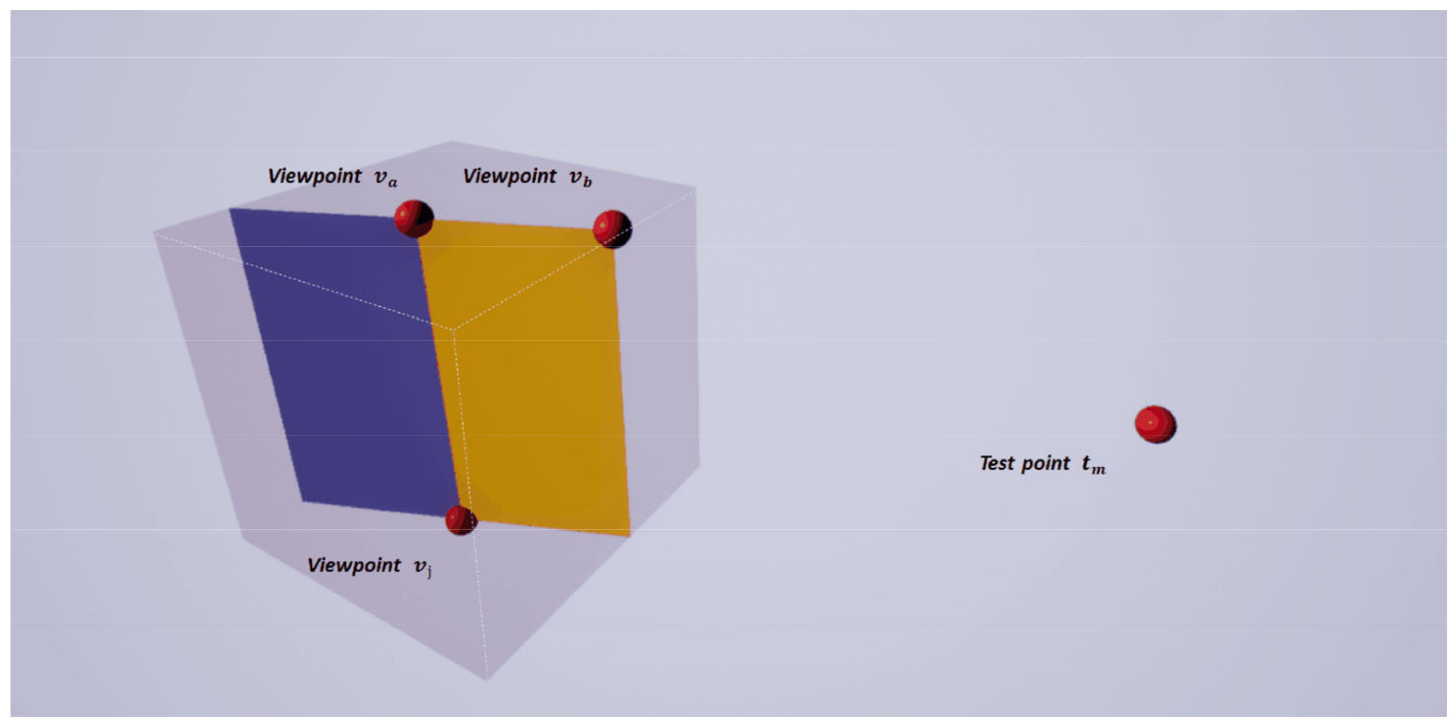
According to the above two properties, viewpoints on the closer edges are more likely to be visible from a test point. Moreover, according to the contrapositive of the two properties, as is shown in Figure 5, if is not visible from , any viewpoint on the orange plane or on the blue plane is also not visible from . If is not visible from , any viewpoint on the blue plane is also not visible from . Suppose in a cell, when we have enough viewpoints from which a test point is invisible, we then assert that the test point is invisible from that cell. The viewpoints located on an edge and closer to a test point are more valuable than other viewpoints because these viewpoints can prove that a wider range of viewpoints are invisible. It can be said that these points are representative, and we call them key points. Similarly, when a test point is higher than the top plane of a cell, we choose key points on the further edges.
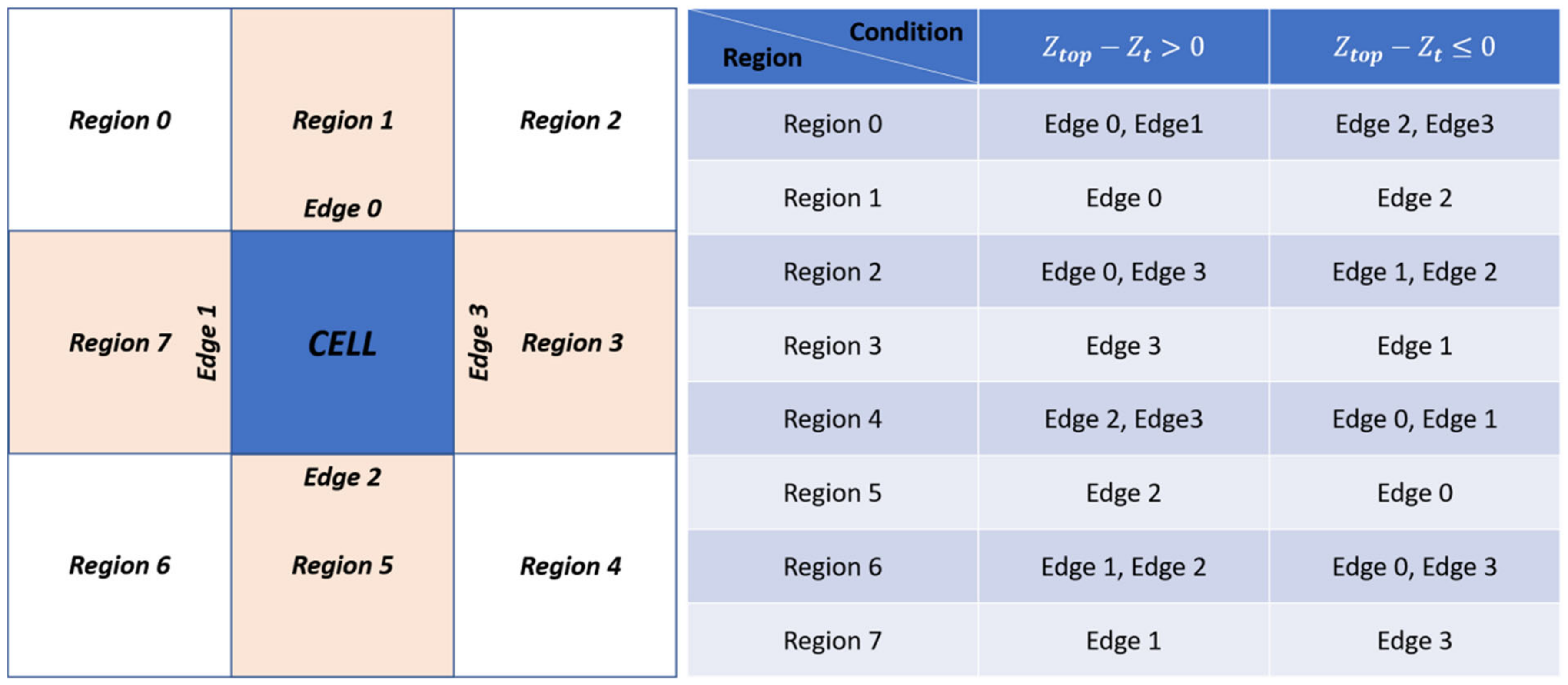
As a strategy, we choose key viewpoints on different edges according to the azimuth, and height of the test point as is shown in Figure 6. When the top plane is higher than the test point, the edges we choose are the edges which are closer to this test point. When the top plane is lower than the test point, the edges we choose are the edges which are further to this test point. These situations are listed in Figure 6.
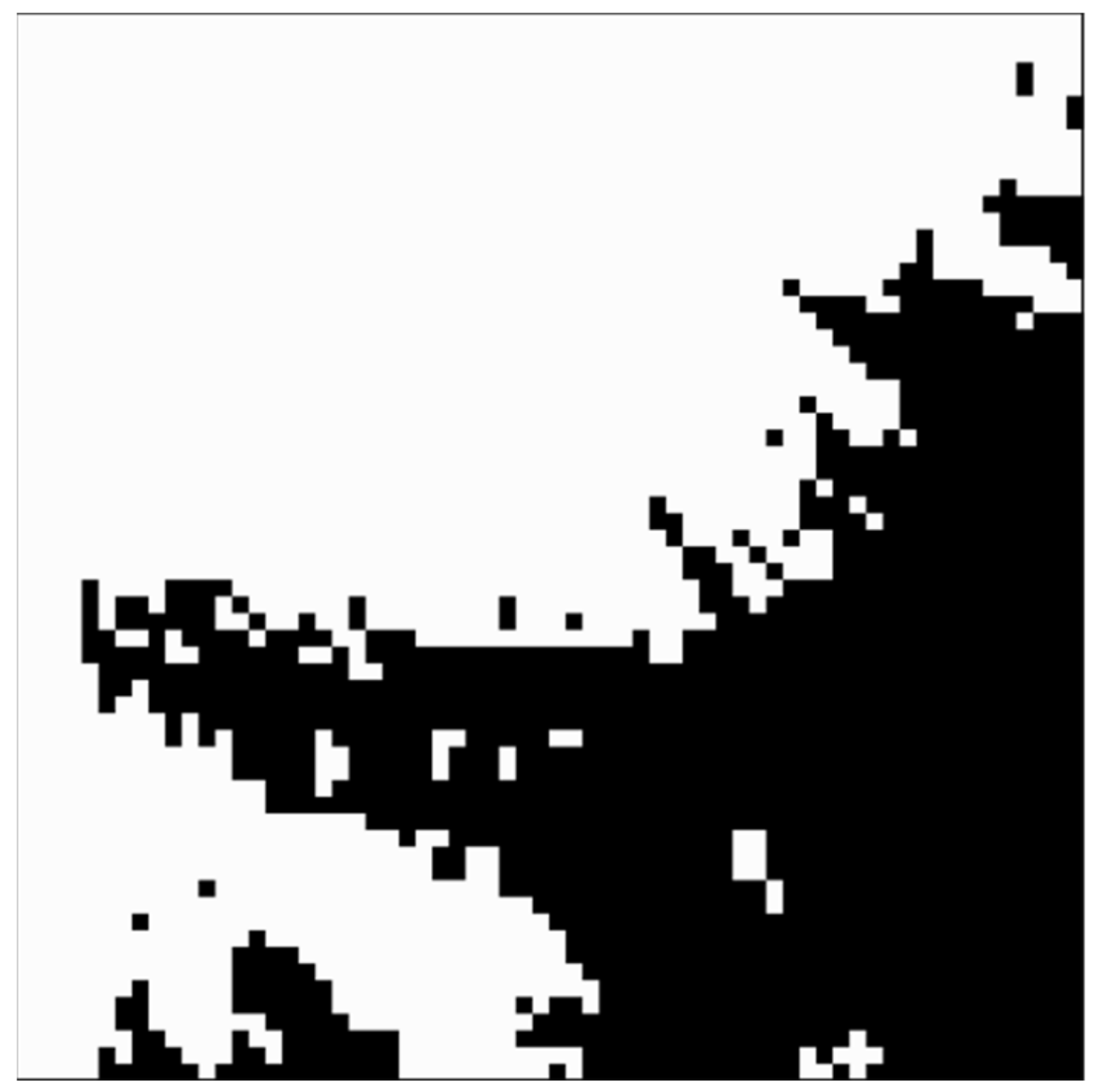
To calculate a test point’s visibility to a cell, we adopt an iterative strategy, first choosing key viewpoints on both ends of the edges and then testing their visibility with the test point: if there is a visible result with the test point, we regard the test point visible from this cell. If all results are false, we choose the midpoint of every two adjacent key viewpoints as new key viewpoints and iterate the above process until reaching a set number of key viewpoints. The larger the number is set, the more accurate the result will be. We set this number to 16 in this paper. Afterward, if all results turn out invisible, we consider this test point is not visible from the cell. We do this for all test points in a patch until we find a visible result. Only when all test points are turn out invisible do we regard this patch as not visible from this cell. The results are Boolean in nature, with 0 corresponding to invisible patches and 1 to visible ones. When the patch is regarded visible from a cell, the corresponding pixel is white; when the patch is regarded invisible from a cell, the pixel is black. All the results form a binary image. Figure 7 shows a cell’s PVPS result.
2.2.3. Roughness Map Computation
We use terrain roughness as a factor to decide quadtree LOD levels. In Digital Terrain Analysis, one of its definitions is the ratio of terrain surface area to projection area [28]. Roughness of a square DEM cell is calculated by Equation (5), where represents the slope of this square DEM cell. Slope is determined by the rates of change (delta) of the surface in the horizontal and vertical directions from the center cell. The values of the center cell and its eight neighbors determine the horizontal and vertical deltas. is calculated by the Slope tool of ArcGIS 10.3.
The computation result is normalized to a range of 0–255 and stored in a grayscale image (Figure 8).
2.3. Initialization and Patches Update
Our method is implemented based on Open Graphics Library (OpenGL). In the sections that follow, we use a right-handed system, where Y is the vertical axis and X and Z are the horizontal axes to keep consistent with OpenGL.
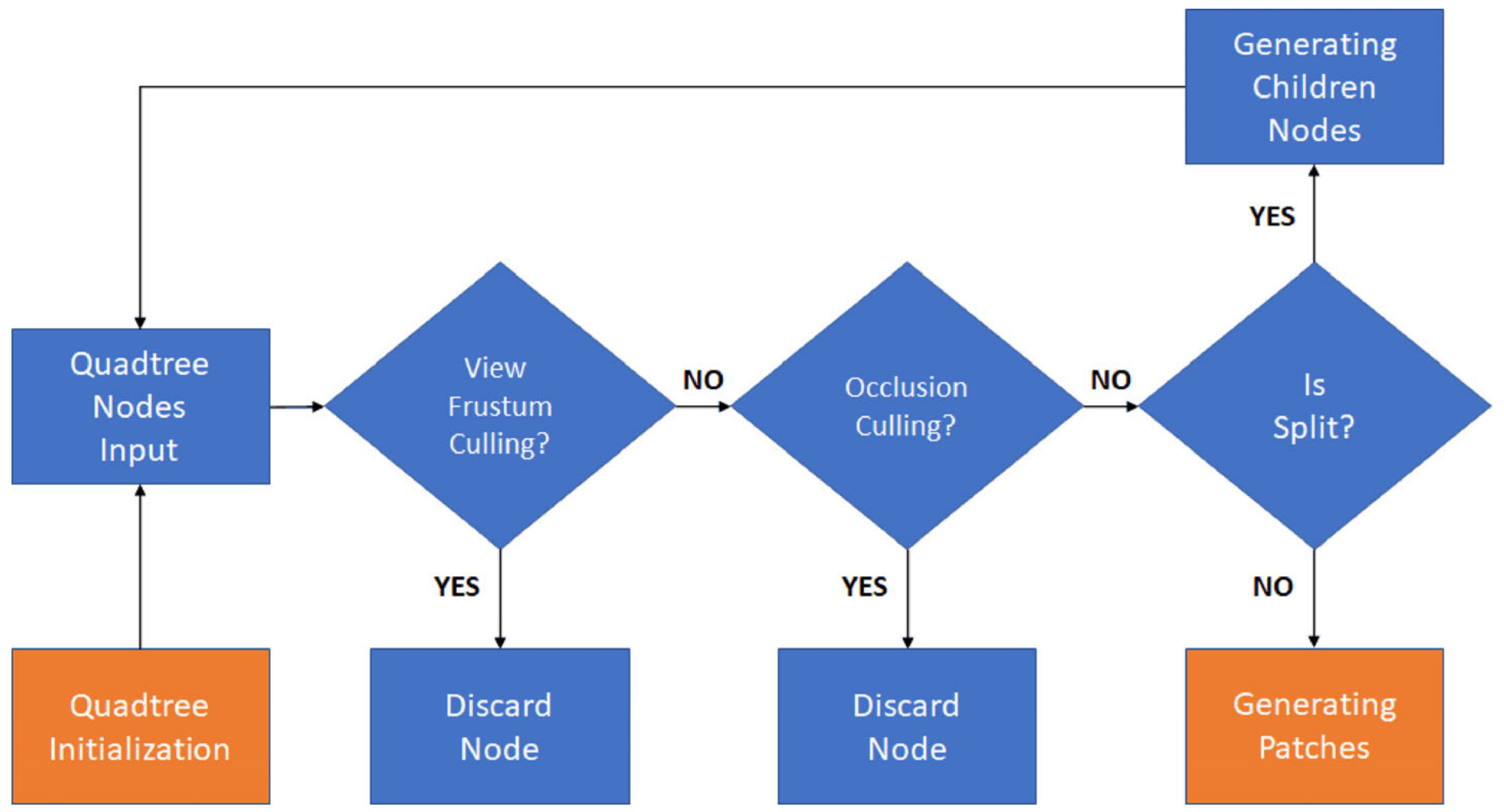
We use a top–down quadtree to generate patches and construct terrain model. The detailed process of initialization and patches update is shown in Figure 9. The whole quadtree construction begins from an initial quadtree node. The initial quadtree node is located at the center of the whole terrain. After it is input, it will be tested for view frustum culling and occlusion culling. The initial quadtree node can almost always split into child quadtree nodes. Child quadtree nodes repeat the same process until all quadtree nodes generate patches.
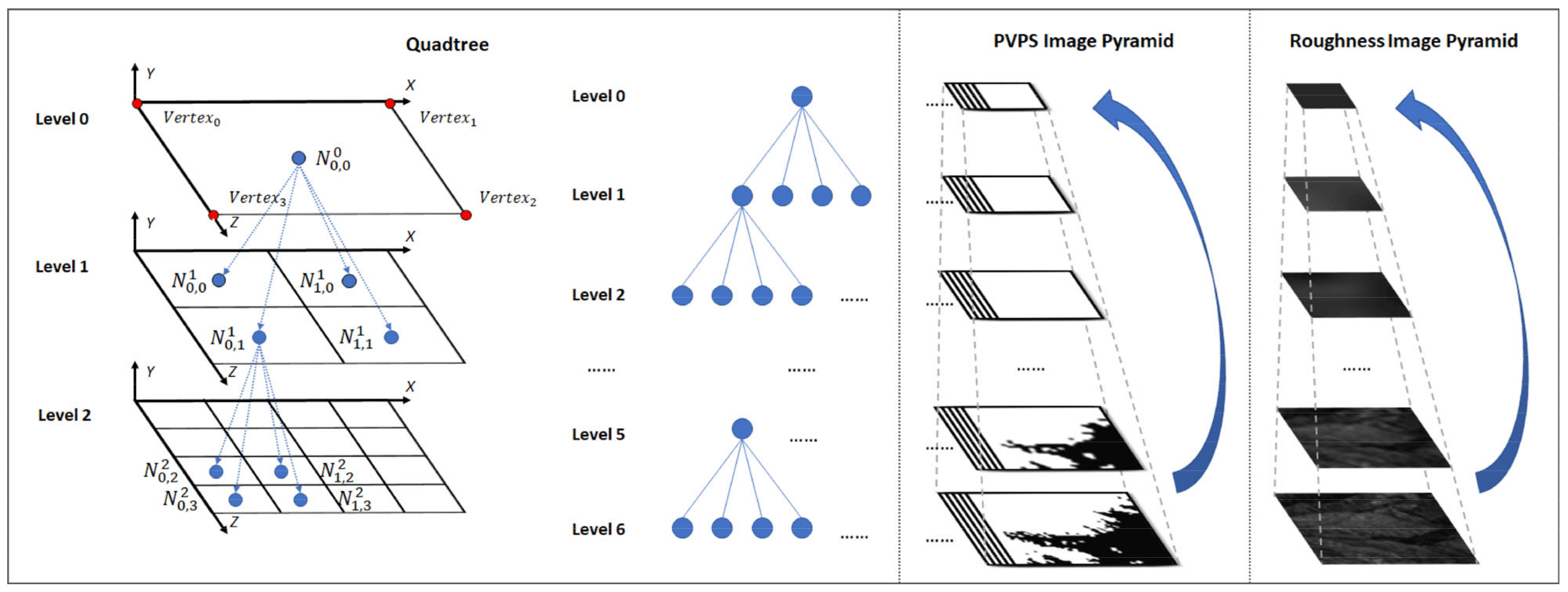
As is shown in Figure 10, a terrain is represented by a group of quadtree nodes. Each quadtree node represents a quadrilateral patch. Quadtree nodes at different levels represent patches of different sizes. We use to represent a quadtree node. represents the level this quadtree node is at. and are used to uniquely determine the location of a quadtree node. represents the ordinal number of the quadtree node counting from the X-axis. represents the ordinal number of the quadtree node counting from the Z-axis.
The coordinates of a quadtree node on the X and Z axes and can be calculated as the following equations. Length represents the length of a patch in coordinate system. For example, as is shown in Figure 10, the Length of the patch generated by is the distance between and .
2.3.1. Quadtree Initialization and Quadtree Nodes Input
At the initialization stage, we first load visibility information. We create PVPS Image Pyramids to store the visibility information. It is used to cull primitives that cannot be culled by view frustum culling. Figure 10 shows a PVPS Image Pyramid and a Roughness Image Pyramid. They have seven levels in total. Each level has PVPS images, and they correspond to cells. Each level has only one roughness image. At level 6, there are quadtree nodes. The PVPS images and roughness image at level six are grayscale images. A lower-level image is half the edge length of the image on the level directly above it.
Each node corresponds to a pixel in the PVPS images and a pixel in the roughness images. A pixel in the PVPS Images represents the visibility of a quadtree node. Each node can find its own visibility information in the PVPS images. There are two grayscale values in PVPS Images A grayscale value 0 (black) represents an invisible node, and a grayscale value 255 (white) represents a visible one. The grayscale value of a pixel in its image is the result of logic OR operation of four neighborhood pixel values in the image of a higher level. Therefore, if any child node of a father quadtree node is visible, the father node is considered visible, and its corresponding pixel value is 255 (white). If all child nodes are invisible, their father node is considered invisible, and the pixel value is 0 (black). Except for pixels in the level six, each pixel in a roughness image is the arithmetic mean of four neighborhood pixel values in the image of a higher level. Before rendering, PVPS images and roughness images are read into memory.
When the quadtree construction begins, the initial quadtree node at LOD level 0 is firstly input. is located at the center of the whole terrain, as is shown in Figure 10.
2.3.2. View Frustum Culling
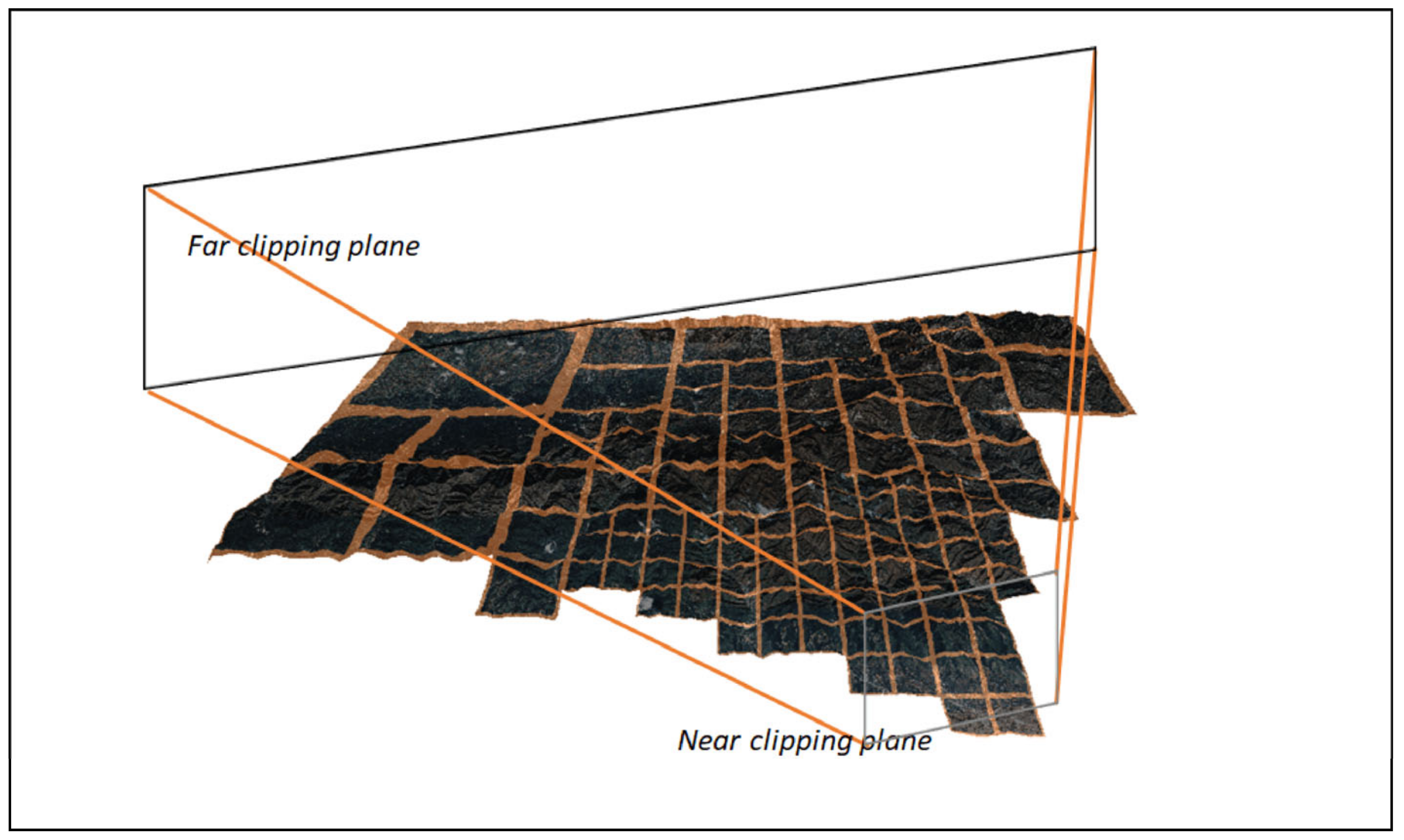
View frustum culling is an idea to cull groups of triangles before GPU stage. It can improve the rendering efficiency as a result. Luna introduced this method and gave an example [9]. In this paper, we build a bounding box for each quadtree node. If the bounding box is outside the frustum, we discard this quadtree node. If the bounding box is inside or intersect the frustum, this quadtree node will become a candidate for being checked for occlusion culling. As is shown in Figure 11, the terrain is composed of different-size patches, which are generated by quadtree nodes. Quadtree nodes not inside the frustum are discarded and do not generate patches.
2.3.3. Occlusion Culling
At this stage, each input quadtree node is checked for PVPS culling. According to the input node’s level and position, we read the pixel value in the corresponding PVPS images. For example, is a quadtree node at level k; it corresponds to a size PVPS image of level k. We read the pixel value at (m,n) of this image. If the pixel value is 0, we determine that this quadtree node is visible, and this quadtree node becomes a candidate for splitting. If the pixel value is 255, we determine that this quadtree node is invisible and discard this node.
2.3.4. Quadtree Nodes Splitting
We use the following equation as a node evaluation function to decide whether a quadtree node splits or not.
is the precomputed roughness value. and are adjustment coefficients. is used to determine the degree of subdivision of the terrain, and is used to determine the influence degree of the terrain roughness to . represents the node’s distance to camera; represents the corresponding terrain edge length of the node. If a quadtree node ’s ratio is lower than 1, it will be split into four child nodes: , , , and , and those four child nodes are tested for view frustum culling in the next iteration. If not splitting, a node will generate a patch. A patch is defined by the coordinates of its four corners, as shown in Equation (10). Their Y-axis coordinates should be the same; here, we set it to 0.
2.4. Rendering
After the iteration process at the CPU ends, coordinates of all patches are sent to GPU. At the GPU stage, input axis-aligned quad patches are tessellated into meshes of geometric primitives [29]. Afterward, a height map texture (Figure 2a) is sampled, and the vertices of meshes are positioned according to the height map.
An important step at this point is how to avoid cracks, a problem that arises when adjacent patches have different sizes. Figure 12a,b shows a terrain with cracks. Because the triangles that make up the terrain do not fit together tightly, some holes and cracks are created.
There are already some methods to solve this problem. Yusov et al. [15] exploit “vertical skirts”, which can hide possible cracks but create extra triangles. Cantlay [17] adds explicit information about a patch’s neighbors. He achieves crack-free terrain by adjusting tessellation factors according to the adjacency information. This method needs to pass additional adjacency information to GPU. Zhang et al. put forward dynamic stitching strips [30]; this is relatively complex for adding extra strips. Kang et al. obtain a crack-free terrain by restricting patch LODs to , i.e., 1, 2, 4, 8, 16, 32, and 64 [19]. Most of these crack-free methods mainly focus on adjusting tessellation scale factor in the Tessellation Control Shader.
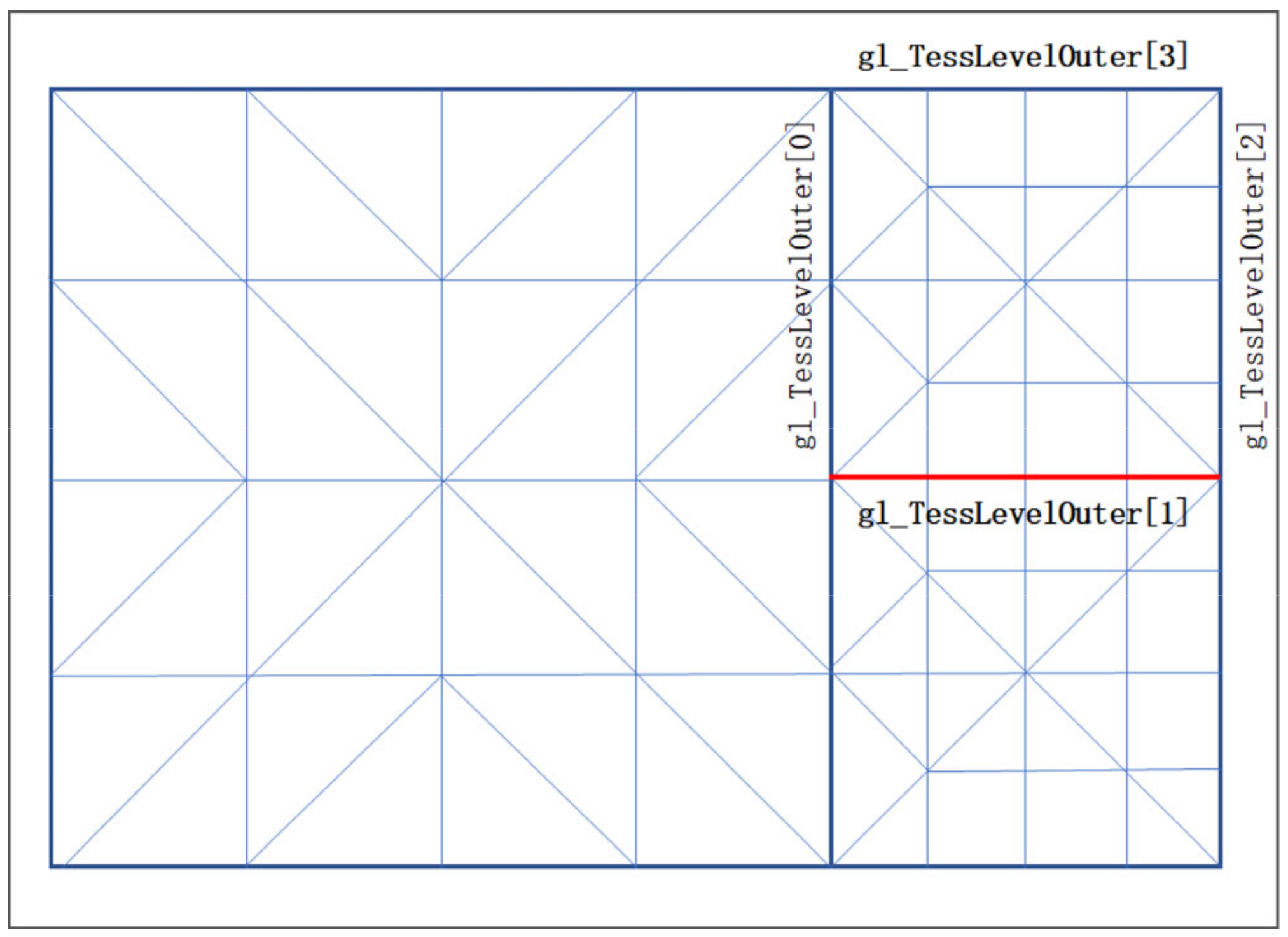
To solve this problem, we divide edges of patches into two class: edges adjacent to different-sized patches and edges adjacent to the same-sized patches. As in shown in Figure 13, the LOD level of the patch in the left is one lower than the two patches in the right. Edges adjacent to patches of the same LOD level are marked red; other edges are marked blue. In addition, edges adjacent to no patches are seen as edges adjacent to different-sized patches.
When the quadtree is computed, we search a node’s four neighbors and calculate their difference in levels. We take advantage of Y-axis coordinates of vertexes to pass classification information of edges without extra data. Coordinates of a patch’s four corners are modified as Equation (11); , , , and represent the LOD levels of a patch’s four neighbors. In the Tessellation Control Shader, Y-axis coordinates of four vertices are used to decided four outer tessellation levels: .
In the Tessellation Control Shader, when the value of Y-axis coordinates of . equals 0, is set as the ratio of the current edge length to the minimum edge length. Minimum edge represents edges of patches, which is generated by quadtree nodes at level six. If the value of Y-axis coordinates of does not equal 0, is up to the edge length in the screen space. The pseudo code is shown in Algorithm 1.
| Algorithm 1 Crack-Free Process. |
|
Constant represents a constant that is used to decide the degree of subdivision of a terrain. Inner tessellation levels are calculated for the number of tessellations within an abstract patch. They are calculated as Equation (12). and present two inner tessellation levels. and represent two edge lengths in the screen space; represents the roughness value, which is obtained by reading roughness maps. and are adjustment coefficients. is used to determine the degree of subdivision of the patch, and is used to determine the influence degree of the roughness value to inner tessellation levels. After setting these tessellation factors, Y-axis coordinates of four corners of the patch are set the original value, for example 0, and passed to tessellation evaluation shader.
3. Results
We perform our experiments in OpenGL 4.6 on a 3.00 GHz Intel Core i7 9700 CPU with an NVIDIA GeForce GTX 1660Ti GPU. The screen resolution is .
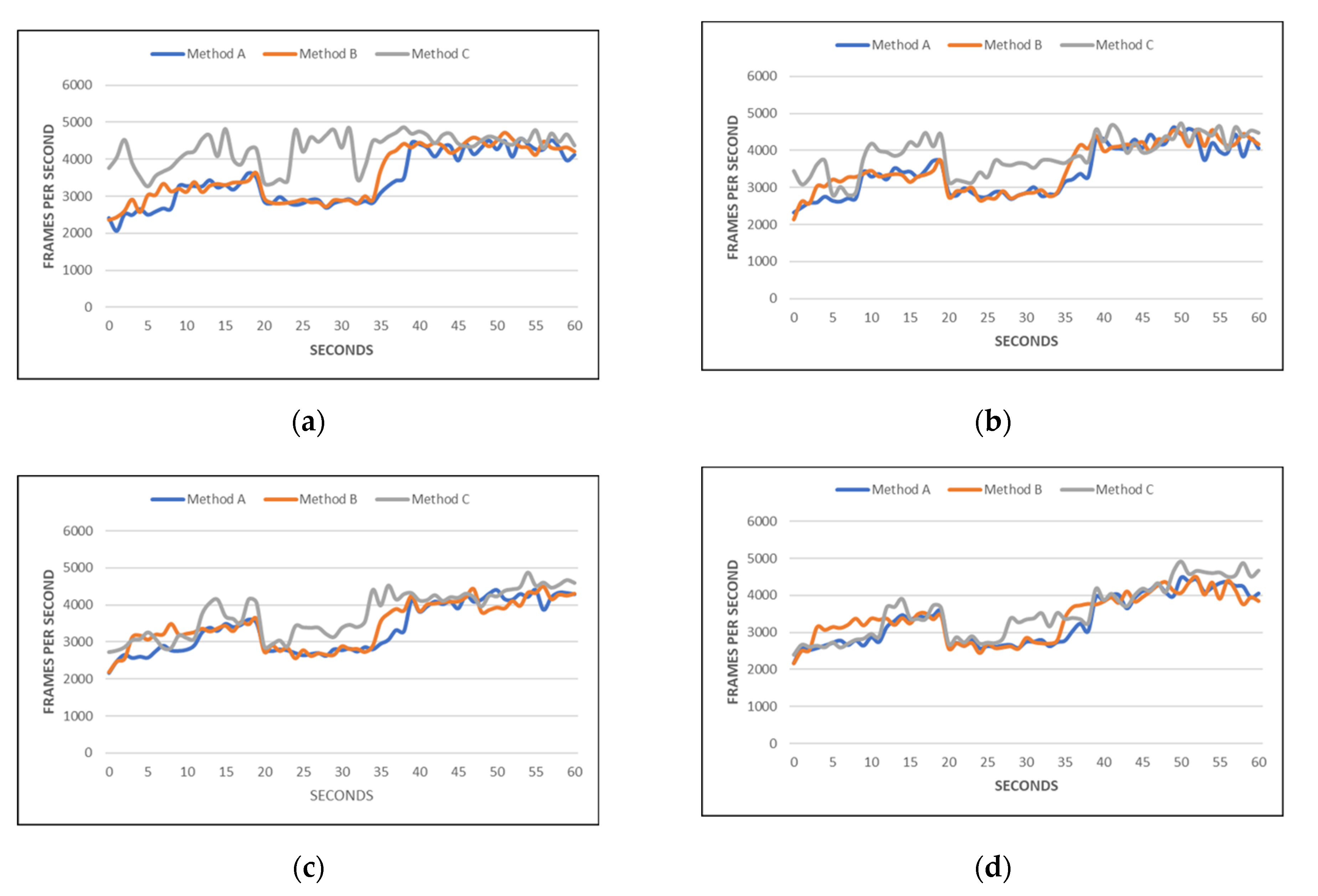
In order to test the effectiveness of our method, we compare the performance of our method with our implementations of two other methods. Figure 14 shows the results of a 60 s flight over the test area at four different heights with method A, method B, and method C. Method A is implemented in Zhai [18]; it is based on quadtrees, and it also takes terrain roughness into consideration. Method B is implemented in Dong [21]. In this method, roughness is defined as the difference between maximum and minimum elevation of a terrain. Method C is the method proposed in this paper. The average camera heights of our experiments are 884 m, 1012 m, 1140 m, and 1268 m. The adjustment parameters and in Equation (12) are set to 10 and 1, respectively. The results are shown in Figure 14a–d and Table 2, respectively. The horizontal axis in Figure 14 represents the timeline of 60 s flights.
Figure 14a shows that PVPS culling can effectively increase the frame rate at an average camera height of 884 m. Compared with the two other methods, the average frame rate increases by 24% and 20%. Table 2 shows the average number of patches and average number of triangles during four flights. When the average camera (viewpoint) position is 884 m, compared with method B and method C, PVPS culling reduces about 24 and 36 patches sent to GPU every frame, and as a result, the number of triangles is reduced effectively.
By comparing the line charts in Figure 14, we can find that the effect of PVPS culling is strongly influenced by the camera (viewpoint) position. We calculate the average frame rate of three methods at different heights as is shown in Table 2. At 884 m, the average frame rate is improved by 834 FPS and 712 FPS compared with method A and method B. However, the average frame rate is only improved by 253 FPS and 165 FPS at 1268 m. As the camera height increases, PVPS culling has less and less effect on improving the rendering frame rate. In summary, PVPS culling can achieve a better performance improvement at lower heights. When the viewpoint is at a high position with a wide field of view, PVPS culling has little improvement in the rendering frame rate.
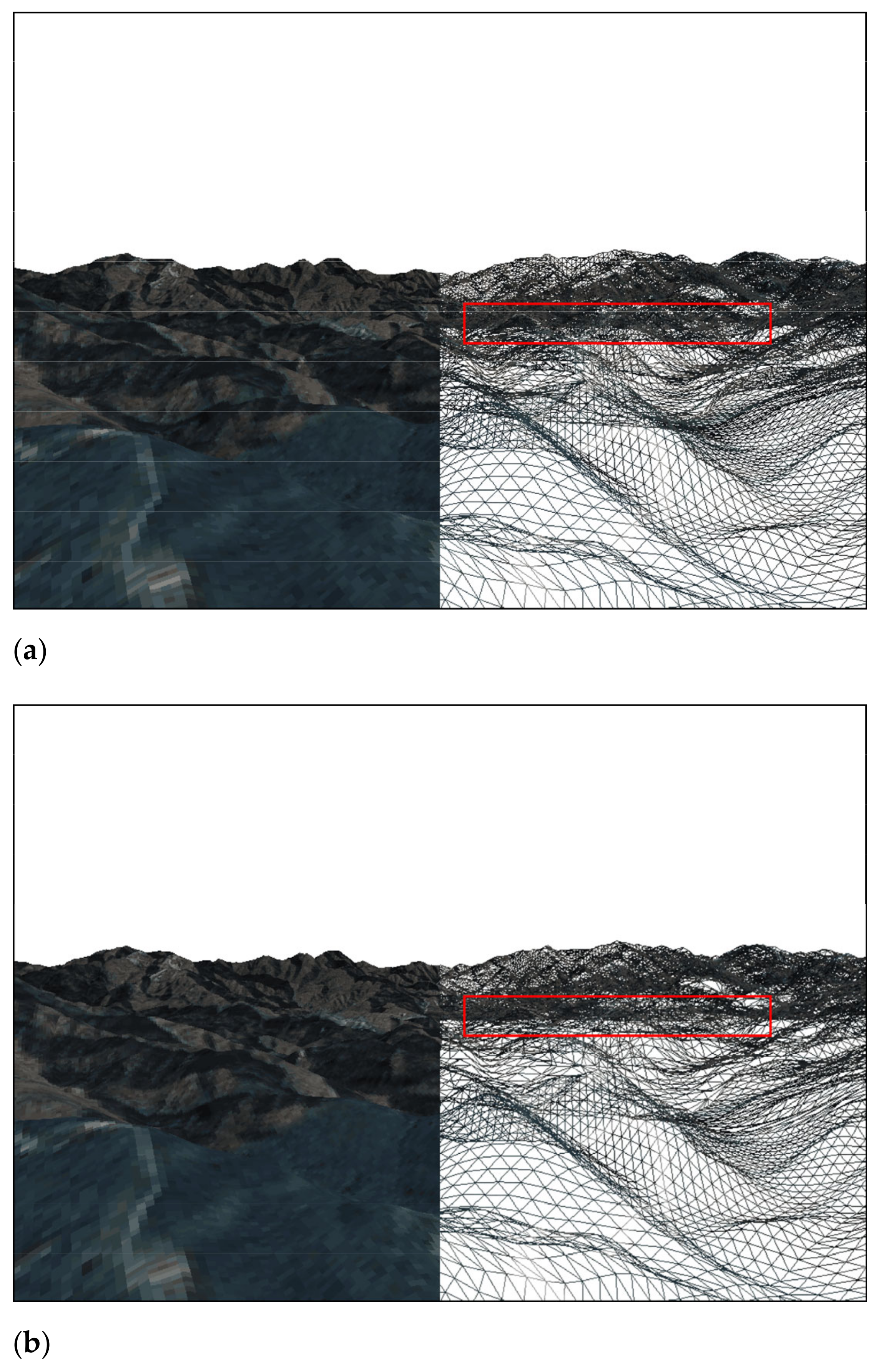
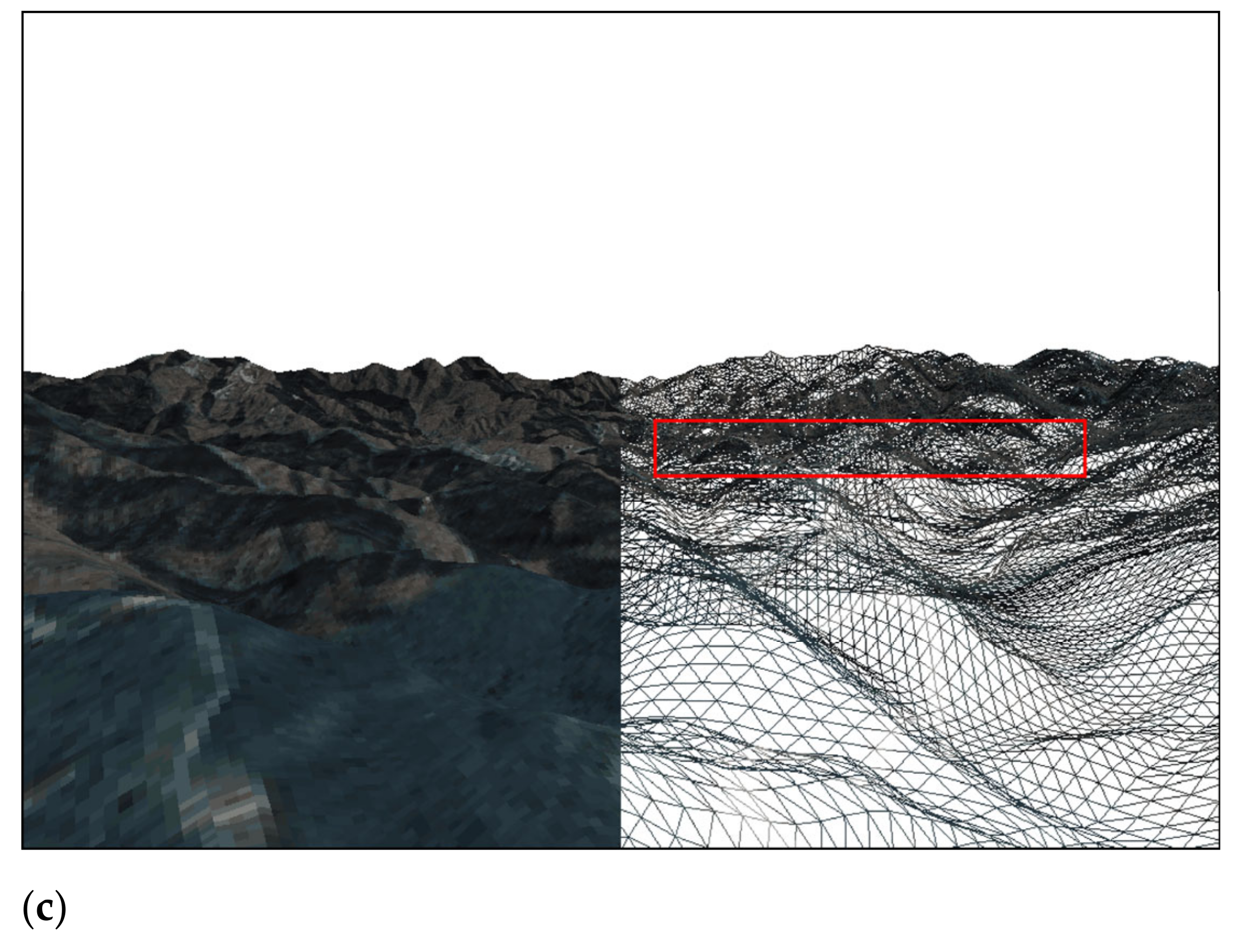
Figure 15 is a set of images that show a frame image of each method. Figure 15a–c show a frame image of method A, method B, and method C, respectively. The difference between the rendered results is not easy to detect. As is shown in the red rectangle, some extra triangles are rendered in method A and method B. Triangles from distant, invisible terrains and triangles from closer terrains coincide. Method C increase the rendering frame rate through rejecting those invisible triangles. Rejecting those triangles does not decrease the density and number of triangles drawn on the screen, ultimately, so the quality of images does not decline.
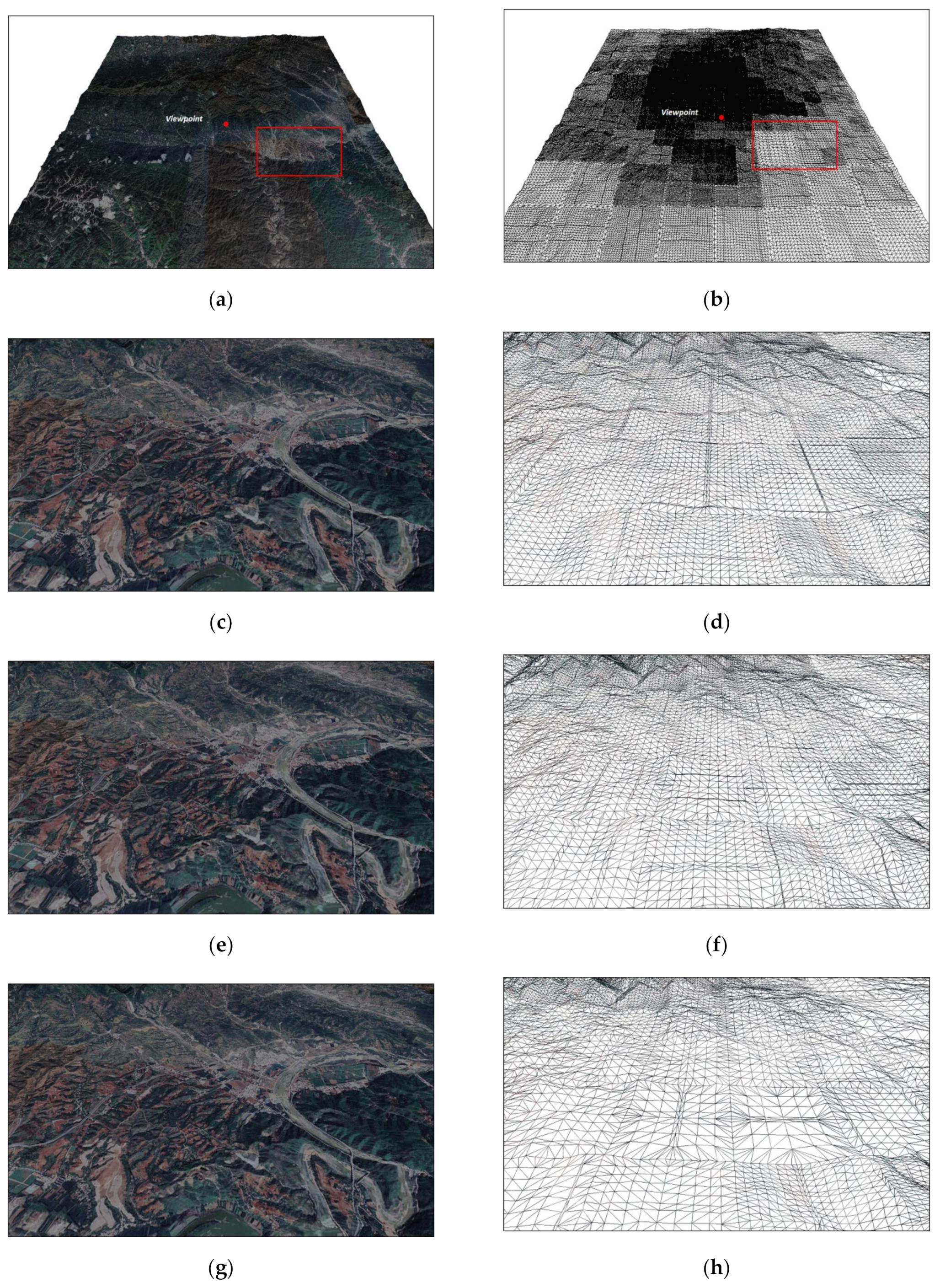
Terrain LOD is indispensable for efficient rendering. Flat terrain needs fewer triangles. As is shown in Figure 16a,b, the camera (viewpoint) is at the center of the terrain; according to the distance to the camera and terrain roughness value, patches are of different Levels of Detail (LOD).
We adjust the subdivision degree of rough terrain by adjusting the adjustment parameters and in Equation (12). The terrain with different roughness can be subdivided into different degrees by taking appropriate adjusting coefficients. We select a typical region to verify the effect of different adjustment coefficients on terrain rendering. The region is in the gentle valley, as is shown in the red rectangle in Figure 16a,b. Figure 16c–h show the influence of different adjustment coefficients over the rendering result of the area. The adjustment coefficients and in Equation (12) are listed in Table 3. In Figure 16d, flat terrain nearby and rugged terrain in the distance show the difference of surface subdivision. These adjustment coefficients are determined by users and influence the number of triangles and, therefore, the FPS. Table 3 shows their impact in this respect. By decreasing the value of and increasing the value of , the number of triangles rendered are reduced, and the frame rate is increased.
Using fewer triangles to render flat terrain has almost no effect on the rendering quality. Through comparison of Figure 16c,e,g, it is difficult to find the difference of the rendering results with different numbers of triangles. By adjusting the subdivision degree of rough terrain using adjustment parameters and , our method can achieve higher frame rates while losing little flat terrain detail.
4. Conclusions and Future Work
This paper presents a method which uses Digital Terrain Analysis to optimize real-time terrain rendering based on hardware tessellation. Digital Terrain Analysis is an important function of Geographic Information Systems. It provides methods to extract terrain features. Our method here employed focuses on mining the features of the terrain itself and uses this information set to optimize rendering process. We introduce the concept of PVPS Image Pyramid and Roughness Image Pyramid and use them for node’s discarding and splitting of terrain quadtree nodes. Our method is based on the viewpoint’s position. According to the PVPS and roughness images of different viewpoint positions, we dynamically adjust the rendering strategy. PVPS Image Pyramid provides a method to cull invisible quadtree nodes hierarchically. Roughness Image Pyramid can help control the degree of terrain division and, therefore, reduce the number of triangles in flat terrains. Calculation of terrain feature information may take too much time, so we precomputed this part of the data. The whole precomputation process takes about 6.5 h in our experiment. We use popular and widely used hardware tessellation technology to achieve rendering results and check the rendering efficiency. Compared with previous methods, our proposed method can improve the rendering performance in different degrees according to the position of the viewpoint. Our proposed method can obtain better rendering performance at lower camera flight heights. As the camera height increases, our method has less and less effect on improving the rendering frame rate.
As a limitation, our method is not effective for flat terrain, where the field of vision is wide and there is almost no self-occlusion. Another limitation of the presented approach is the space partitioning into regular cells, which leads to a lack of flexibility. In future work, we will try to partition the space into irregular cells according to the situation of terrain self-occlusion. In addition, we will also use more terrain features for LOD selection and compare the differences between them. Application of the proposed method on larger terrains is also under consideration.
Author Contributions
Conceptualization, Lei Zhang; software, Lei Zhang and Wenjun Feng; data curation, Ping Wang and Chengyi Huang; writing—original draft preparation, Lei Zhang; writing—review and editing, Lei Zhang and Bo Ai; visualization, Lei Zhang; funding acquisition, Bo Ai. All authors have read and agreed to the published version of the manuscript.
Funding
This work was supported by the National Natural Science Foundation of China [Grant No. 62071279, 41930535] and the SDUST Research Fund [Grant No. 2019TDJH103].
Acknowledgments
The authors would like to thank the editors and anonymous reviewers for their meaningful comments and helpful suggestions.
Conflicts of Interest
The authors declare no conflict of interest.
References
- Petrie, G.; Kennie, T.J.M. Terrain modelling in surveying and civil engineering. Comput.-Aided Des. 1987, 19, 171–187. [Google Scholar] [CrossRef]
- Baumann, K.; Doellner, J.; Hinrichs, K.H.; Kersting, O. A Hybrid, Hierarchical Data Structure for Real-Time Terrain Visualization. In Proceedings of the Computer Graphics International, Canmore, Alta, Canada, 11 June 1999; IEEE: Picataway, NJ, USA, 1999; pp. 85–92. [Google Scholar]
- Boo, M.; Amor, M. Dynamic hybrid terrain representation based on convexity limits identification. Int. J. Geogr. Inf. Sci. 2009, 23, 417–439. [Google Scholar] [CrossRef]
- Paredes, E.G.; Bóo, M.; Amor, M.; Döllner, J.; Bruguera, J.D. GPU-based Visualization of Hybrid Terrain Models. In Proceedings of the GRAPP/IVAPP, Rome, Italy, 24–26 February 2012; pp. 254–259. [Google Scholar]
- Hoppe, H. Progressive meshes. In Proceedings of the 23rd Annual Conference on Computer Graphics and Interactive Techniques; ACM Press: Boston, MA, USA, 1996; pp. 99–108. [Google Scholar]
- Hoppe, H. View-dependent refinement of progressive meshes. In Proceedings of the 24th Annual Conference on Computer Graphics and Interactive Techniques, Los Angeles, CA, USA, 3–8 August 1997; ACM Press: Boston, MA, USA, 1997; pp. 189–198. [Google Scholar]
- Duchaineau, M.; Wolinsky, M.; Sigeti, D.E.; Miller, M.C.; Aldrich, C.; Mineev-Weinstein, M.B. ROAMing terrain: Real-time optimally adapting meshes. In Proceedings. Visualization’97 (Cat. No. 97CB36155); IEEE: Piscataway, NJ, USA, 1997; pp. 81–88. [Google Scholar]
- Ulrich, T. Rendering massive terrains using chunked level of detail control. In Proc. ACM SIGGRAPH 2002; Association for Computing Machinery: New York, NY, USA, 2002. [Google Scholar]
- Luna, F. Introduction to 3D Game Programming with DirectX 12; Stylus Publishing, LLC: Sterling, VA, USA, 2016. [Google Scholar]
- Lindstrom, P.; Pascucci, V. Terrain simplification simplified: A general framework for view-dependent out-of-core visualization. IEEE Trans. Vis. Comput. Graph. 2002, 8, 239–254. [Google Scholar] [CrossRef]
- Ripolles, O.; Ramos, F.; Puig-Centelles, A.; Chover, M. Real-time tessellation of terrain on graphics hardware. Comput. Geosci. 2012, 41, 147–155. [Google Scholar] [CrossRef] [Green Version]
- Livny, Y.; Kogan, Z.; El-Sana, J. Seamless patches for GPU-based terrain rendering. Vis. Comput. 2009, 25, 197–208. [Google Scholar] [CrossRef] [Green Version]
- Luna, F. Introduction to 3D Game Programming with DirectX 11; Stylus Publishing, LLC: Sterling, VA, USA, 2012. [Google Scholar]
- Schäfer, H.; Niessner, M.; Keinert, B.; Stamminger, M.; Loop, C.T. State of the Art Report on Real-time Rendering with Hardware Tessellation. In Eurographics (State of the Art Reports); EUROGRAPHICS Association: Goslar, Germany, 2014; pp. 93–117. [Google Scholar]
- Yusov, E.; Shevtsov, M. High-performance terrain rendering using hardware tessellation. WSCG 2011, 19, 85–92. [Google Scholar]
- Engel, W. (Ed.) GPU Pro 4: Advanced Rendering Techniques; CRC Press: Boca Raton, FL, USA, 2013. [Google Scholar]
- Cantlay, I. Directx 11 Terrain Tessellation. Nvidia Whitepaper 2011, 8, 3. [Google Scholar]
- Zhai, R.; Lu, K.; Pan, W.; Dai, S. GPU-based real-time terrain rendering: Design and implementation. Neurocomputing 2016, 171, 1–8. [Google Scholar] [CrossRef]
- Kang, H.; Jang, H.; Cho, C.S.; Han, J. Multi-resolution terrain rendering with GPU tessellation. Vis. Comput. 2015, 31, 455–469. [Google Scholar] [CrossRef]
- Fu, H.; Yang, H.; Chen, C. Large-scale terrain-adaptive LOD control based on GPU tessellation. Alex. Eng. J. 2021, 60, 2865–2874. [Google Scholar] [CrossRef]
- Dong, L.; Zhang, B.; Zhao, X. A Seamless Terrain Rendering Algorithm Based on GPU Tessellation; Geomatics and Information Science of Wuhan University; Wuhan University: Wuhan, China, 2017. [Google Scholar]
- Airey, J.M.; Rohlf, J.H.; Brooks Jr, F.P. Towards image realism with interactive update rates in complex virtual building environments. ACM SIGGRAPH Comput. Graph. 1990, 24, 41–50. [Google Scholar] [CrossRef] [Green Version]
- Laakso, M. Potentially Visible Set (PVS); Helsinki University of Technology: Espoo, Finland, 2003. [Google Scholar]
- Durand, F. A Multidisciplinary Survey of Visibility. In ACM Siggraph Course Notes Visibility, Problems, Techniques, and Applications; Association for Computing Machinery: New York, NY, USA, 2000. [Google Scholar]
- Zaugg, B.; Egbert, P.K. Voxel column culling: Occlusion culling for large terrain models. In Data Visualization; Springer: Vienna, Austria, 2001; pp. 85–93. [Google Scholar]
- Floriani, L.; Magillo, P. Algorithms for visibility computation on terrains: A survey. Environ. Plan. B Plan. Des. 2003, 30, 709–728. [Google Scholar] [CrossRef] [Green Version]
- Bresenham, J.E. Algorithm for computer control of a digital plotter. IBM Syst. J. 1965, 4, 25–30. [Google Scholar] [CrossRef]
- Chorley, R.J. Spatial Analysis in Geomorphology; Routledge: Oxfordshire, UK, 2019; pp. 3–16. [Google Scholar]
- Kessenich, J.; Sellers, G.; Shreiner, D. OpenGL Programming Guide: The Official Guide to Learning Opengl, Version 4.5 with SPIR-V; Addison-Wesley Professional: Boston, MA, USA, 2016. [Google Scholar]
- Zhang, L.; She, J.; Tan, J.; Wang, B.; Sun, Y. A multilevel terrain rendering method based on dynamic stitching strips. ISPRS Int. J. Geo-Inf. 2019, 8, 255. [Google Scholar] [CrossRef] [Green Version]
Figure 1.
Process of our method.

Figure 2.
Diagram of the terrain and partitions. (a) represents the terrain height map, a TIFF 32-bit, sampled at 12.5 m spacing, grayscale image. (b) represents the partition result, partitioned into patches. (c) shows the scene’s partition, in addition to partitions on the plane; it is partitioned in the vertical direction.


Figure 3.
Diagram of 3D Bresenham algorithm and line-of-sight algorithm. (a) describes 3D Bresenham algorithm. The blue line segment is the projection of the line segment formed by two points on the terrain. The gray grids are the grids through which the line segments pass. The black points are the intersections of the vertical lines from the center of the gray grids to the blue line segment. A black point’s elevation value is represented by the elevation value of the nearest DEM cell. (b) shows line-of-sight algorithms we use. The blue line represents the terrain section line.

Figure 4.
Test points. There are test points in total.

Figure 5.
Diagram of the positional relationship between points.

Figure 6.
Diagram of edge selection policy. The picture on the left shows the top view of a cell. The possible areas of all test points are divided into 8 regions. A test point may be located at one of 8 different regions. represents the elevation of the top plane of a cell; represents elevation of the test point. Our viewpoints are sampled on the top plane of a cell; their elevations are the same. According to 2 different conditions, as is shown in the table, samples will be taken on different edges.

Figure 7.
Diagram of a PVPS map. A PVPS map is a binary image. Potential visible patches are marked white, and not visible ones are marked black.
Figure 7.
Diagram of a PVPS map. A PVPS map is a binary image. Potential visible patches are marked white, and not visible ones are marked black.

Figure 8.
Diagram of a terrain roughness map. It is a grayscale image.

Figure 9.
Flowchart of quadtree initialization and patches update.

Figure 10.
Diagram of the quadtree, PVPS Image Pyramid, and Roughness Image Pyramid. Blue circles represent quadtree nodes, and red circles represents corners of a patch.
Figure 10.
Diagram of the quadtree, PVPS Image Pyramid, and Roughness Image Pyramid. Blue circles represent quadtree nodes, and red circles represents corners of a patch.

Figure 11.
The terrain after view frustum culling.

Figure 12.
A terrain with cracks. (a,b) show a terrain with cracks. The cracks are marked by red rectangles. (c,d) show the result of our crack-free method.
Figure 12.
A terrain with cracks. (a,b) show a terrain with cracks. The cracks are marked by red rectangles. (c,d) show the result of our crack-free method.

Figure 13.
Diagram of edges of two classes.

Figure 14.
Comparison among different methods. (a) Average camera heights of 884 m. (b) Average camera heights of 1012 m. (c) Average camera heights of 1140 m. (d) Average camera heights of 1268 m.
Figure 14.
Comparison among different methods. (a) Average camera heights of 884 m. (b) Average camera heights of 1012 m. (c) Average camera heights of 1140 m. (d) Average camera heights of 1268 m.

Figure 15.
Frame images of three methods. (a) shows a frame image of Method A. (b) shows a frame image of Method B. (c) shows a frame image of Method C.
Figure 15.
Frame images of three methods. (a) shows a frame image of Method A. (b) shows a frame image of Method B. (c) shows a frame image of Method C.


Figure 16.
Influence of different adjustment parameters on terrain subdivision. (a,b) show the region we select to verify the effect of different adjustment parameters. (c,d) = 10, = 1. (e,f) = 12.5, = 0.5. (g,h) = 15, = 0.25.
Figure 16.
Influence of different adjustment parameters on terrain subdivision. (a,b) show the region we select to verify the effect of different adjustment parameters. (c,d) = 10, = 1. (e,f) = 12.5, = 0.5. (g,h) = 15, = 0.25.


Table 1.
Comparison of the various methods.
| Method | Grid-Based/Triangulation-Based/Hybrid | Levels Of Detail (LOD) | Quadtree/Binary Tree | GPU Tessellation | View Frustum Culling | Occlusion Culling |
|---|---|---|---|---|---|---|
| Baumann [2] | Hybrid | Yes | No | No | Yes | No |
| Paredes [4] | Hybrid | Yes | No | Yes | No | No |
| Hoppe [5] | Triangulation | Yes | No | No | No | No |
| Duchaineau [7] | Triangulation | Yes | Binary Tree | No | No | No |
| Ulrich [8] | Grid | Yes | Quadtree | No | No | No |
| Ripolles [11] | Grid | No | No | Yes | No | No |
| Yusov [15] | Grid | Yes | Quadtree | Yes | No | No |
| Engel [16] | Procedural Algorithm | Yes | Quadtree | Yes | Yes | No |
| Cantlay [17] | Grid | Yes | No | Yes | No | No |
| Zhai [18] | Grid | Yes | Quadtree | Yes | Yes | No |
| Kang [19] | Grid | Yes | Quadtree | Yes | No | No |
| Fu [20] | Grid | Yes | Quadtree | Yes | Yes | No |
| DONG [21] | Grid | Yes | Quadtree | Yes | Yes | No |
| Zaugg [25] | Grid | Yes | Quadtree | No | No | Yes |
| Ours | Grid | Yes | Quadtree | Yes | Yes | Yes |
Table 2.
Comparison among different methods.
| Average Camera Heights (m) | Methods | Average Frame Rate (Frame/s) | Average Number of Patches | Average Number of Triangles |
|---|---|---|---|---|
| 884 | Method A | 3445 | 92 | 115,269 |
| Method B | 3567 | 104 | 110,194 | |
| Method C | 4279 | 68 | 79,063 | |
| 1012 | Method A | 3433 | 91 | 116,540 |
| Method B | 3521 | 103 | 112,497 | |
| Method C | 3884 | 73 | 89,391 | |
| 1140 | Method A | 3357 | 90 | 117,139 |
| Method B | 3444 | 102 | 116,505 | |
| Method C | 3764 | 81 | 102,119 | |
| 1268 | Method A | 3304 | 88 | 118,157 |
| Method B | 3392 | 101 | 117,094 | |
| Method C | 3557 | 83 | 105,194 |
Table 3.
Comparison of different adjustment coefficients.
| Adjustment Parameters | Number of Triangles | Frame Rate (Frame/s) |
|---|---|---|
| = 10, = 1 | 112,868 | 1921 |
| = 12.5, = 0.5 | 72,314 | 2223 |
| = 15, = 0.25 | 83,470 | 2295 |
Publisher’s Note: MDPI stays neutral with regard to jurisdictional claims in published maps and institutional affiliations. |
© 2021 by the authors. Licensee MDPI, Basel, Switzerland. This article is an open access article distributed under the terms and conditions of the Creative Commons Attribution (CC BY) license (https://creativecommons.org/licenses/by/4.0/).
Share and Cite
MDPI and ACS Style
Zhang, L.; Wang, P.; Huang, C.; Ai, B.; Feng, W. A Method of Optimizing Terrain Rendering Using Digital Terrain Analysis. ISPRS Int. J. Geo-Inf. 2021, 10, 666. https://0-doi-org.brum.beds.ac.uk/10.3390/ijgi10100666
AMA Style
Zhang L, Wang P, Huang C, Ai B, Feng W. A Method of Optimizing Terrain Rendering Using Digital Terrain Analysis. ISPRS International Journal of Geo-Information. 2021; 10(10):666. https://0-doi-org.brum.beds.ac.uk/10.3390/ijgi10100666
Chicago/Turabian StyleZhang, Lei, Ping Wang, Chengyi Huang, Bo Ai, and Wenjun Feng. 2021. "A Method of Optimizing Terrain Rendering Using Digital Terrain Analysis" ISPRS International Journal of Geo-Information 10, no. 10: 666. https://0-doi-org.brum.beds.ac.uk/10.3390/ijgi10100666
Note that from the first issue of 2016, this journal uses article numbers instead of page numbers. See further details here.