
Quantification of Loess Landforms from Three-Dimensional Landscape Pattern Perspective by Using DEMs

 ,
,  and
and
Abstract
:1. Introduction
2. Materials and Methods
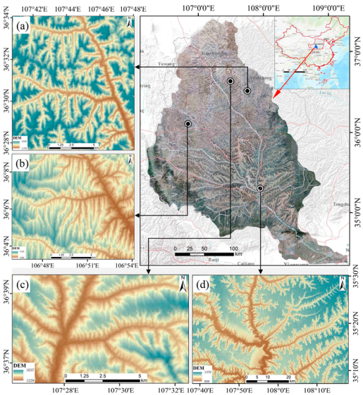
2.1. Study Area
2.2. Data Sources
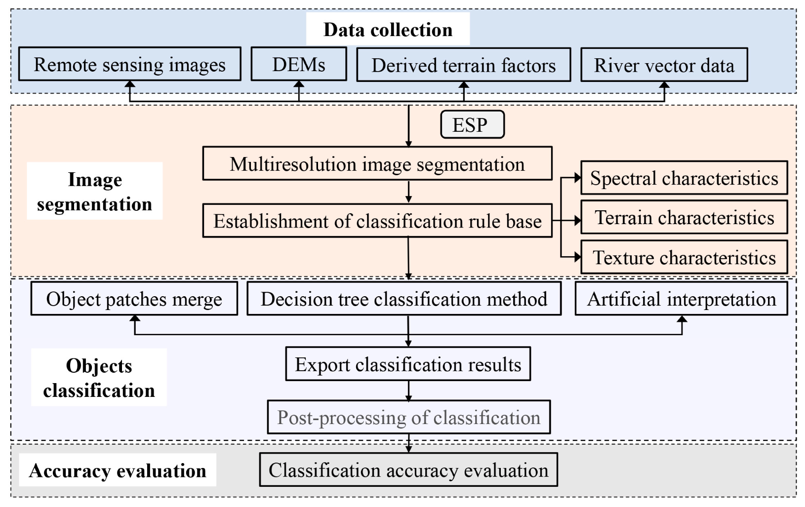
2.3. Methods
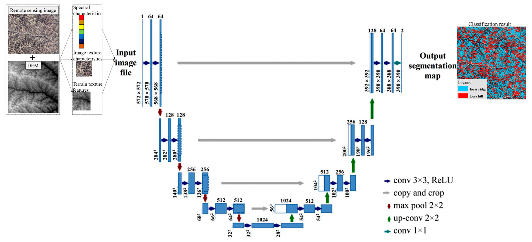
2.3.1. Loess Landform Types Extraction
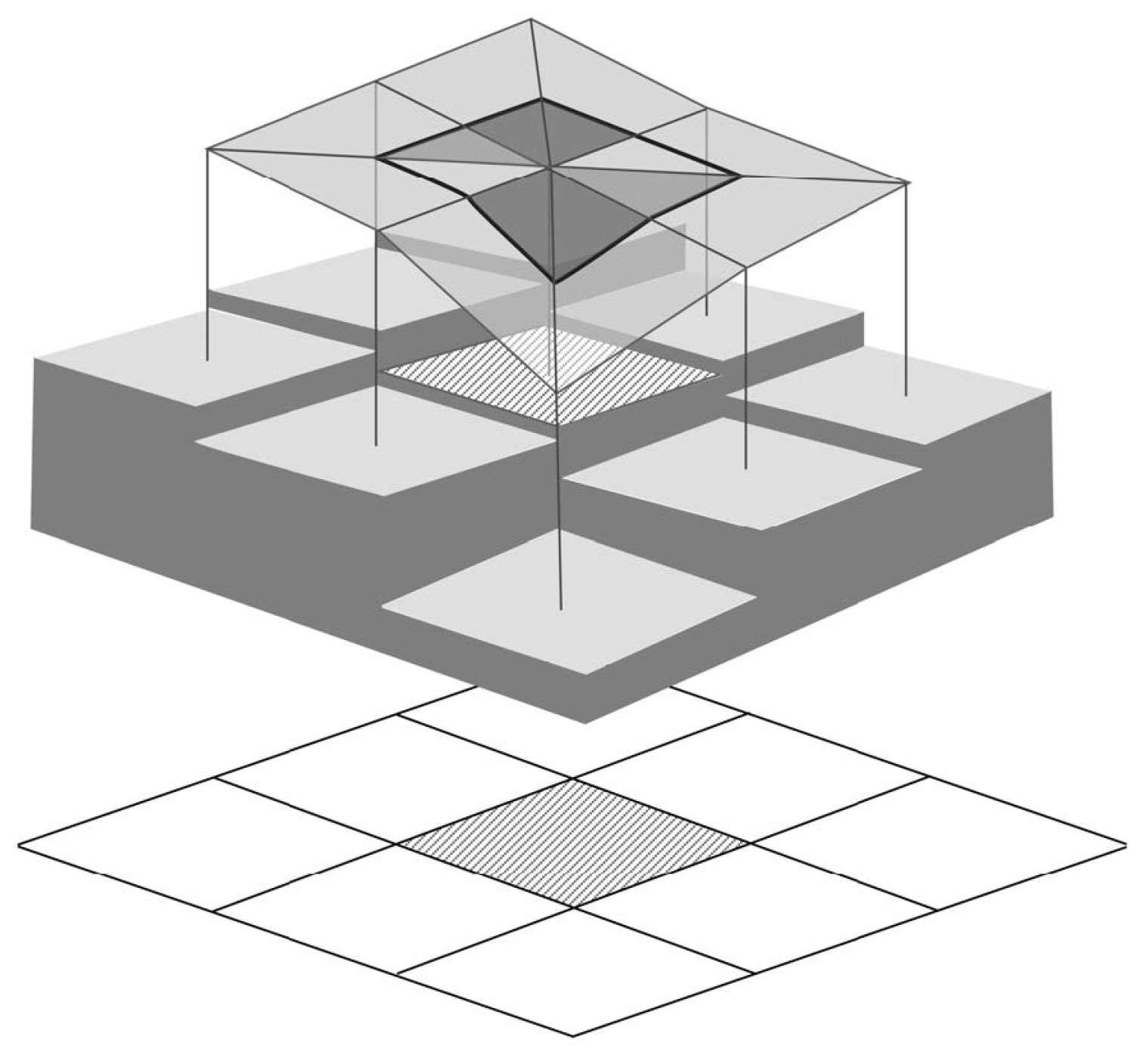
2.3.2. 3D Landscape Pattern Indices
3. Results
3.1. Extracted Loess Landform Types
3.2. Calculated Quantitative Indices
4. Discussion
4.1. Comparison of Loess Landform Classification Methods
4.2. Sensitivity of the 3D Landscape Pattern Indices to Topography
4.3. Analysis of Evolution Process between Loess Landform Types
4.4. Limitations and Future Research
5. Conclusions
Author Contributions
Funding
Data Availability Statement
Acknowledgments
Conflicts of Interest
References
- Vandenbruwaene, W.; Schwarz, C.; Bouma, T.; Meire, P.; Temmerman, S. Landscape-scale flow patterns over a vegetated tidal marsh and an unvegetated tidal flat: Implications for the landform properties of the intertidal floodplain. Geomorphology 2015, 231, 40–52. [Google Scholar] [CrossRef]
- Duque, J.M.; Zapico, I.; Oyarzun, R.; García, J.L.; Cubas, P. A descriptive and quantitative approach regarding erosion and development of landforms on abandoned mine tailings: New insights and environmental implications from SE Spain. Geomorphology 2015, 239, 1–16. [Google Scholar] [CrossRef] [Green Version]
- MacMillan, R.; Pettapiece, W.; Nolan, S.; Goddard, T. A generic procedure for automatically segmenting landforms into landform elements using DEMs, heuristic rules and fuzzy logic. Fuzzy Set Syst. 2000, 113, 81–109. [Google Scholar] [CrossRef]
- Irvin, B.J.; Ventura, S.J.; Slater, B.K. Fuzzy and isodata classification of landform elements from digital terrain data in Pleasant Valley, Wisconsin. Geoderma 1997, 77, 137–154. [Google Scholar] [CrossRef]
- Feng, L.; Lin, H.; Zhang, M.; Guo, L.; Jin, Z.; Liu, X. Development and evolution of Loess vertical joints on the Chinese Loess Plateau at different spatiotemporal scales. Eng. Geol. 2020, 265, 105372. [Google Scholar] [CrossRef]
- Li, Y.; Shi, W.; Aydin, A.; Beroya-Eitner, M.A.; Gao, G. Loess genesis and worldwide distribution. Earth-Sci. Rev. 2020, 201, 102947. [Google Scholar] [CrossRef]
- Xiong, L.; Tang, G.; Li, F.; Yuan, B.; Lu, Z. Modeling the evolution of loess-covered landforms in the Loess Plateau of China using a DEM of underground bedrock surface. Geomorphology 2014, 209, 18–26. [Google Scholar] [CrossRef]
- Wu, Z.; Zhao, D.; Che, A.; Chen, D.; Liang, C. Dynamic response characteristics and failure mode of slopes on the loess tableland using a shaking-table model test. Landslides 2020, 1561–1575. [Google Scholar] [CrossRef]
- Xiong, L.; Tang, G.; Yang, X.; Li, F. Geomorphology-oriented digital terrain analysis: Progress and perspectives. J. Geogr. Sci. 2021, 31, 456–476. [Google Scholar] [CrossRef]
- Kennelly, P.J. Terrain maps displaying hill-shading with curvature. Geomorphology 2008, 102, 567–577. [Google Scholar] [CrossRef]
- Cheng, Y.; Yang, X.; Liu, H.; Li, M.; Rossiter, D.G.; Xiong, L.; Tang, G. Computer-assisted terrain sketch mapping that considers the geomorphological features in a loess landform. Geomorphology 2020, 364, 107169. [Google Scholar] [CrossRef]
- Du, L.; You, X.; Li, K.; Meng, L.; Cheng, G.; Xiong, L.; Wang, G. Multi-modal deep learning for landform recognition. ISPRS J. Photogramm. Remote Sens. 2019, 158, 63–75. [Google Scholar] [CrossRef]
- Xiong, L.; Zhu, A.; Zhang, L.; Tang, G. Drainage basin object-based method for regional-scale landform classification: A case study of loess area in China. Phys. Geogr. 2018, 39, 523–541. [Google Scholar] [CrossRef]
- Zhao, F.; Xiong, L.; Wang, C.; Wang, H.; Wei, H.; Tang, G. Terraces mapping by using deep learning approach from remote sensing images and digital elevation models. Trans. GIS 2021, 1–17. [Google Scholar] [CrossRef]
- Hu, G.; Dai, W.; Li, S.; Xiong, L.; Tang, G. A vector operation to extract second-order terrain derivatives from digital elevation models. Remote Sens. 2020, 12, 3134. [Google Scholar] [CrossRef]
- Fang, H.; Cai, Q.; Chen, H.; Li, Q. Effect of rainfall regime and slope on runoff in a gullied loess region on the Loess Plateau in China. Environ. Manag. 2008, 42, 402–411. [Google Scholar] [CrossRef]
- Cao, M.; Tang, G.a.; Zhang, F.; Yang, J. A cellular automata model for simulating the evolution of positive–negative terrains in a small loess watershed. Int. J. Geogr. Inf. Sci. 2013, 27, 1349–1363. [Google Scholar] [CrossRef]
- Jiang, C.; Fan, W.; Yu, N.; Nan, Y. A New Method to Predict Gully Head Erosion in the Loess Plateau of China Based on SBAS-InSAR. Remote Sens. 2021, 13, 421. [Google Scholar] [CrossRef]
- Yuan, S.; Xu, Q.; Zhao, K.; Wang, X.; Wang, C. Geomorphological classification and evolution of plateau-beam-loess hills in Heshui county of the east Gansu province. Geogr. Res. 2020, 39, 1920–1933. [Google Scholar]
- Pike, R.J.; Wilson, S.E. Elevation-relief ratio, hypsometric integral, and geomorphic area-altitude analysis. Geol. Soc. Am. Bull. 1971, 82, 1079–1084. [Google Scholar] [CrossRef]
- Ding, H.; Na, J.; Jiang, S.; Zhu, J.; Liu, K.; Fu, Y.; Li, F. Evaluation of Three Different Machine Learning Methods for Object-Based Artificial Terrace Mapping—A Case Study of the Loess Plateau, China. Remote Sens. 2021, 13, 1021. [Google Scholar] [CrossRef]
- Blaschke, T. Object based image analysis for remote sensing. ISPRS J. Photogramm. Remote Sens. 2010, 65, 2–16. [Google Scholar] [CrossRef] [Green Version]
- Li, X.; Cheng, X.; Chen, W.; Chen, G.; Liu, S. Identification of forested landslides using LiDar data, Object-based image analysis, and machine learning algorithms. Remote Sens. 2015, 7, 9705–9726. [Google Scholar] [CrossRef] [Green Version]
- Feizizadeh, B.; Blaschke, T.; Tiede, D.; Moghaddam, M.H.R. Evaluating fuzzy operators of an object-based image analysis for detecting landslides and their changes. Geomorphology 2017, 293, 240–254. [Google Scholar] [CrossRef]
- Myint, S.W.; Gober, P.; Brazel, A.; Grossman-Clarke, S.; Weng, Q. Per-pixel vs. object-based classification of urban land cover extraction using high spatial resolution imagery. Remote Sens. Environ. 2011, 115, 1145–1161. [Google Scholar] [CrossRef]
- Zhao, W.; Xiong, L.; Ding, H.; Tang, G. Automatic recognition of loess landforms using Random Forest method. J. Mt. Sci. 2017, 14, 885–897. [Google Scholar] [CrossRef]
- Dingle Robertson, L.; King, D.J. Comparison of pixel-and object-based classification in land cover change mapping. Int. J. Remote Sens. 2011, 32, 1505–1529. [Google Scholar] [CrossRef]
- Stevens, T.; Carter, A.; Watson, T.; Vermeesch, P.; Andò, S.; Bird, A.; Lu, H.; Garzanti, E.; Cottam, M.; Sevastjanova, I. Genetic linkage between the Yellow River, the Mu Us desert and the Chinese loess plateau. Quat. Sci. Rev. 2013, 78, 355–368. [Google Scholar] [CrossRef]
- Rinaldo, A.; Rodriguez-Iturbe, I.; Rigon, R.; Bras, R.L.; Ijjasz-Vasquez, E.; Marani, A. Minimum energy and fractal structures of drainage networks. Water Resour. Res. 1992, 28, 2183–2195. [Google Scholar] [CrossRef]
- Huang, X.; Tang, G.; Zhu, T.; Ding, H.; Na, J. Space-for-time substitution in geomorphology. J. Geogr. Sci. 2019, 29, 1670–1680. [Google Scholar] [CrossRef] [Green Version]
- Wu, H.; Xu, X.; Zheng, F.; Qin, C.; He, X. Gully morphological characteristics in the loess hilly-gully region based on 3D laser scanning technique. Earth Surf. Proc. Land 2018, 43, 1701–1710. [Google Scholar] [CrossRef]
- Xiong, L.; Tang, G. Research progresses and prospects of gully landform formation and evolution in the Loess Plateau of China. J. Geo-Inf. Sci. 2020, 22, 816–826. [Google Scholar]
- Kramm, T.; Hoffmeister, D.; Curdt, C.; Maleki, S.; Khormali, F.; Kehl, M. Accuracy assessment of landform classification approaches on different spatial scales for the Iranian loess plateau. ISPRS Int. J. Geo-Inf. 2017, 6, 366. [Google Scholar] [CrossRef] [Green Version]
- Li, S.; Xiong, L.; Tang, G.; Strobl, J. Deep learning-based approach for landform classification from integrated data sources of digital elevation model and imagery. Geomorphology 2020, 354, 107045. [Google Scholar] [CrossRef]
- Li, P.; Mu, X.; Holden, J.; Wu, Y.; Irvine, B.; Wang, F.; Gao, P.; Zhao, G.; Sun, W. Comparison of soil erosion models used to study the Chinese Loess Plateau. Earth-Sci. Rev. 2017, 170, 17–30. [Google Scholar] [CrossRef] [Green Version]
- Sun, W.; Shao, Q.; Liu, J.; Zhai, J. Assessing the effects of land use and topography on soil erosion on the Loess Plateau in China. Catena 2014, 121, 151–163. [Google Scholar] [CrossRef]
- Ma, S.; Qiu, H.; Hu, S.; Pei, Y.; Yang, W.; Yang, D.; Cao, M. Quantitative assessment of landslide susceptibility on the Loess Plateau in China. Phys. Geogr. 2020, 41, 489–516. [Google Scholar] [CrossRef]
- Wu, Y.; Ke, Y.; Chen, Z.; Liang, S.; Zhao, H.; Hong, H. Application of alternating decision tree with AdaBoost and bagging ensembles for landslide susceptibility mapping. Catena 2020, 187, 104396. [Google Scholar] [CrossRef]
- Jasiewicz, J.; Stepinski, T.F. Geomorphons—A pattern recognition approach to classification and mapping of landforms. Geomorphology 2013, 182, 147–156. [Google Scholar] [CrossRef]
- Wei, H.; Xiong, L.; Tang, G.; Strobl, J.; Xue, K. Spatial–temporal variation of land use and land cover change in the glacial affected area of the Tianshan Mountains. Catena 2021, 202, 105256. [Google Scholar] [CrossRef]
- Tischendorf, L. Can landscape indices predict ecological processes consistently? Landsc. Ecol. 2001, 16, 235–254. [Google Scholar] [CrossRef]
- Li, H.; Wu, J. Use and misuse of landscape indices. Landsc. Ecol. 2004, 19, 389–399. [Google Scholar] [CrossRef] [Green Version]
- Petras, V.; Newcomb, D.J.; Mitasova, H. Generalized 3D fragmentation index derived from lidar point clouds. Open Geospat. Data Softw. Stand. 2017, 2, 9. [Google Scholar] [CrossRef] [Green Version]
- Wu, Q.; Guo, F.; Li, H.; Kang, J. Measuring landscape pattern in three dimensional space. Landsc. Urban. Plan. 2017, 167, 49–59. [Google Scholar] [CrossRef]
- Dong, W.; Sullivan, P.; Stout, K. Comprehensive study of parameters for characterizing three-dimensional surface topography: III: Parameters for characterizing amplitude and some functional properties. Wear 1994, 178, 29–43. [Google Scholar] [CrossRef]
- Wang, Z.; Tinh, N.T.; Ma, X.; Yin, J.; Hu, J. Research on extraction of hydrological information in the Jinghe River Basin based on SRTM_DEM. China Rural Water Hydropower 2011, 11, 32–36. [Google Scholar]
- Chen, C.; Xie, G.; Zhen, L.; Leng, Y. Analysis on Jinghe watershed vegetation dynamics and evaluation on its relation with precipitation. Acta Ecol. Sin. 2008, 28, 925–938. [Google Scholar]
- Zhen, L.; Xie, G.; Yang, L.; Cheng, S. Characters of landscape patterns and correlation in Jinghe watershed. Acta Ecol. Sin. 2005, 25, 3343–3353. [Google Scholar]
- Chang, K.; Tsai, B. The effect of DEM resolution on slope and aspect mapping. Cart. Geogr. Inf. 1991, 18, 69–77. [Google Scholar] [CrossRef]
- Feizizadeh, B.; Garajeh, M.K.; Blaschke, T.; Lakes, T. An object based image analysis applied for volcanic and glacial landforms mapping in Sahand Mountain, Iran. Catena 2021, 198, 105073. [Google Scholar] [CrossRef]
- Yan, G.; Mas, J.F.; Maathuis, B.; Xiangmin, Z.; Van Dijk, P. Comparison of pixel-based and object-oriented image classification approaches—a case study in a coal fire area, Wuda, Inner Mongolia, China. Int. J. Remote Sens. 2006, 27, 4039–4055. [Google Scholar] [CrossRef]
- Blaschke, T.; Hay, G.J.; Kelly, M.; Lang, S.; Hofmann, P.; Addink, E.; Feitosa, R.Q.; Van der Meer, F.; Van der Werff, H.; Van Coillie, F. Geographic object-based image analysis–towards a new paradigm. ISPRS J. Photogramm. Remote Sens. 2014, 87, 180–191. [Google Scholar] [CrossRef] [Green Version]
- Drăguţ, L.; Csillik, O.; Eisank, C.; Tiede, D. Automated parameterisation for multi-scale image segmentation on multiple layers. ISPRS J. Photogramm. Remote Sens. 2014, 88, 119–127. [Google Scholar] [CrossRef] [PubMed] [Green Version]
- Janowski, L.; Tylmann, K.; Trzcinska, K.; Rudowski, S.; Tegowski, J. Exploration of Glacial Landforms by Object-Based Image Analysis and Spectral Parameters of Digital Elevation Model. IEEE Trans. Geosci. Remote Sens. 2021. [Google Scholar] [CrossRef]
- Benz, U.C.; Hofmann, P.; Willhauck, G.; Lingenfelder, I.; Heynen, M. Multi-resolution, object-oriented fuzzy analysis of remote sensing data for GIS-ready information. ISPRS J. Photogramm. Remote Sens. 2004, 58, 239–258. [Google Scholar] [CrossRef]
- Drăguţ, L.; Eisank, C.; Strasser, T. Local variance for multi-scale analysis in geomorphometry. Geomorphology 2011, 130, 162–172. [Google Scholar] [CrossRef] [Green Version]
- Drǎguţ, L.; Tiede, D.; Levick, S.R. ESP: A tool to estimate scale parameter for multiresolution image segmentation of remotely sensed data. Int. J. Geogr. Inf. Sci. 2010, 24, 859–871. [Google Scholar] [CrossRef]
- Jenness, J.S. Calculating landscape surface area from digital elevation models. Wildl. Soc. B 2004, 32, 829–839. [Google Scholar] [CrossRef]
- Blaschke, T.; Strobl, J. What’s wrong with pixels? Some recent developments interfacing remote sensing and GIS. Zeitschrift Geoinformationssysteme 2001, 14, 12–17. [Google Scholar]
- Duro, D.C.; Franklin, S.E.; Dubé, M.G. A comparison of pixel-based and object-based image analysis with selected machine learning algorithms for the classification of agricultural landscapes using SPOT-5 HRG imagery. Remote Sens. Environ. 2012, 118, 259–272. [Google Scholar] [CrossRef]
- Zhao, H.; Fang, X.; Ding, H.; Josef, S.; Xiong, L.; Na, J.; Tang, G. Extraction of terraces on the Loess Plateau from high-resolution DEMs and imagery utilizing object-based image analysis. ISPRS Int. J. Geo-Inf. 2017, 6, 157. [Google Scholar] [CrossRef] [Green Version]
- Ma, L.; Li, M.; Ma, X.; Cheng, L.; Du, P.; Liu, Y. A review of supervised object-based land-cover image classification. ISPRS J. Photogramm. Remote Sens. 2017, 130, 277–293. [Google Scholar] [CrossRef]
- Lu, C.; Qi, W.; Li, L.; Sun, Y.; Qin, T.; Wang, N. Applications of 2D and 3D landscape pattern indices in landscape pattern analysis of mountainous area at county level. J. Appl. Ecol. 2012, 23, 1351–1358. [Google Scholar]
- Wu, Z.; Wei, L.; Lv, Z. Landscape pattern metrics: An empirical study from 2-D to 3-D. Phys. Geogr. 2012, 33, 383–402. [Google Scholar] [CrossRef]
- Frohn, R.C.; Hao, Y. Landscape metric performance in analyzing two decades of deforestation in the Amazon Basin of Rondonia, Brazil. Remote Sens. Environ. 2006, 100, 237–251. [Google Scholar] [CrossRef]
- Jia, Y.; Tang, L.; Xu, M.; Yang, X. Landscape pattern indices for evaluating urban spatial morphology–A case study of Chinese cities. Ecol. Indic. 2019, 99, 27–37. [Google Scholar] [CrossRef]
- Schoorl, J.M.; Sonneveld, M.P.W.; Veldkamp, A. Three-dimensional landscape process modelling: The effect of DEM resolution. Earth Surf. Process. Landf. 2000, 25, 1025–1034. [Google Scholar] [CrossRef]
- Hoechstetter, S.; Thinh, N.X.; Walz, U. 3D-indices for the analysis of spatial patterns of landscape structure. In Proceedings of the InterCarto–InterGIS 12. International Conference on Geoinformation for Sustainable Development, Berlin, Germany, 28–30 August 2006; Volume 12, pp. 108–118. [Google Scholar]
- Chen, Z.; Xu, B.; Devereux, B. Urban landscape pattern analysis based on 3D landscape models. Appl. Geogr. 2014, 55, 82–91. [Google Scholar] [CrossRef]
- Du Preez, C. A new arc–chord ratio (ACR) rugosity index for quantifying three-dimensional landscape structural complexity. Landsc. Ecol. 2015, 30, 181–192. [Google Scholar] [CrossRef]
- Stupariu, M.S.; Pàtru-Stupariu, I.G.; Cuculici, R. Geometric approaches to computing 3D-landscape metrics. Landsc. Online 2010, 24, 1–12. [Google Scholar] [CrossRef]
- Cheng, N.; He, H.; Lu, Y.; Yang, S. Coupling analysis of hydrometeorology and erosive landforms evolution in Loess Plateau, China. Adv. Meteorol. 2016. [Google Scholar] [CrossRef] [Green Version]
- Li, J.; Xiong, L.; Tang, G. Combined gully profiles for expressing surface morphology and evolution of gully landforms. Front. Earth Sci. 2019, 13, 551–562. [Google Scholar] [CrossRef]
- Qi, Q.; Chi, T. Research on the theory and method of Geo-Info-TUPU. Acta Geogr. Sin. 2001, 56, 8–18. [Google Scholar]
- Ouyang, W.; Hao, F.; Skidmore, A.K.; Toxopeus, A. Soil erosion and sediment yield and their relationships with vegetation cover in upper stream of the Yellow River. Sci. Total Environ. 2010, 409, 396–403. [Google Scholar] [CrossRef]
- Zhao, G.; Mu, X.; Wen, Z.; Wang, F.; Gao, P. Soil erosion, conservation, and eco-environment changes in the Loess Plateau of China. Land Degrad. Dev. 2013, 24, 499–510. [Google Scholar] [CrossRef]
- Guo, J.; Wang, W.; Shi, J. A quantitative analysis of the stage of geomorphologic evolution in Luohe drainage basin, north of Shaanxi Province. Arid Land Geogr. 2015, 38, 1161–1168. [Google Scholar]
- Tarolli, P. High-resolution topography for understanding Earth surface processes: Opportunities and challenges. Geomorphology 2014, 216, 295–312. [Google Scholar] [CrossRef]


| Data | Resolution | Purpose | Data Sources |
|---|---|---|---|
| DEMs | 12.5 m | Provide terrain information and texture for landform classification | National Aeronautics and Space Administration |
| Remote sensing image | 2.38 m | Provide spectral information and texture for landform classification | Google Earth |
| Slope | 12.5 m | Auxiliary data for landform classification | Calculated from DEMs |
| Aspect | 12.5 m | Auxiliary data for landform classification | Calculated from DEMs |
| River vector data | — | Auxiliary data for image segmentation | Upper and Middle Reaches Administration of the Yellow River |
| Index | Formulation | Formula Description |
|---|---|---|
| Total length of edge (TE) | Ei is the surface edge length of patch i, n is the total number of patches of landform type | This indicator can reflect the total edge length of a particular landform type (unit: km). |
| Mean patch size (MPS) | Ai is the total surface area of loess landform i, and Ni is the total number of patches of landform type i. | This indicator can reflect a specific landform type’s average patch area size (unit: km2). |
| Mean patch fractal dimension (MPFD) | pi is the surface circumference of patch i, ai is the surface area of patch i, n is the total number of patches i. | The value range of MPFD is between 1–2, and the larger the value, the more complex the shape of the patch. |
| Landscape shape index (LSI) | E is the total length of the surface edge of a certain loess landform type, and Ai is the total surface area. | This indicator reflects the elongation of the patch. The larger the value of LSI, the longer the shape of the patch. |
| Circularity index (CI) | Ei is the surface edge length of patch i, ai is the surface area of patch i. | This index is to quantify the shape of the patch. The closer the value is to 1, the closer the patch is to circle. |
| Slope | Calculated in ArcGIS platform | The index represents the topographic features of the patch (°). |
| Edge dimension index (EDI) | pi is the surface circumference of patch i, ai is the surface area of patch i. | This index reflects the complexity of the shape of the patch. |
| Landform Types | Classification Rules | Description |
|---|---|---|
| Loess tableland | (a) Ses = 36, Bri > 134, DEMs > 1335, slo < 7 | The loess tableland is a large and flat plain that remains after the original loess plain is cut by gullies. |
| (d) Ses = 36, Bri > 319, DEMs > 1115, slo < 6 | ||
| Loess ridge | (a) Area < 10 km2, LWR > 3 | The loess ridge is a long strip of high elevation with a long shape and a narrow width. The area is significantly smaller than the loess tableland and surrounded by loess gullies. |
| (b) Ses = 40, area > 1 km2, LWR > 3 | ||
| (c) Ses = 32, area > 0.3 km2 LWR > 2 | ||
| (d) Area < 20 km2, LWR > 5 | ||
| Loess hill | Area < 1 km2, LWR < 2.5, slo < 10° | The loess hill is a round, nearly circular loess mound, an independent patch with an area usually less than 1 km2. |
| Sample | Manually Sketched Area | Correctly Classified Area | Accuracy |
|---|---|---|---|
| a | 17.32 km2 | 15.15 km2 | 87.47% |
| b | 21.46 km2 | 18.52 km2 | 86.3% |
| c | 14.60 km2 | 11.86 km2 | 81.23% |
| d | 28.16 km2 | 26.32 km2 | 93.47% |
| total | 81.54 km2 | 71.85 km2 | 88.12% |
| Sample | TE | MPS | MPFD | LSI | CI | Slope | EDI | |
|---|---|---|---|---|---|---|---|---|
| Sample a | Loess tableland | 97.07 | 12.67 | 1.58 | 6.35 | 1.68 | 5.14 | 11.27 |
| Loess ridge | 14.18 | 2.07 | 1.37 | 2.72 | 2.05 | 4.99 | 7.94 | |
| Loess hill | 1.71 | 0.20 | 1.22 | 0.94 | 1.24 | 6.13 | 2.46 | |
| Sample b | Loess ridge | 3.07 | 1.35 | 1.43 | 1.16 | 1.73 | 5.66 | 5.42 |
| Loess hill | 1.47 | 0.10 | 1.22 | 0.85 | 1.18 | 7.14 | 2.03 | |
| Sample c | Loess ridge | 8.02 | 1.92 | 1.43 | 1.65 | 2.14 | 4.62 | 4.28 |
| Loess hill | 1.61 | 0.13 | 1.18 | 1.13 | 1.37 | 6.22 | 1.72 | |
| Sample d | Loess tableland | 399.23 | 113.95 | 1.42 | 9.43 | 1.46 | 3.01 | 8.47 |
| Loess ridge | 72.86 | 12.52 | 1.33 | 5.41 | 1.44 | 5.72 | 3.38 | |
| Loess hill | 5.65 | 0.22 | 1.24 | 2.46 | 1.14 | 8.32 | 1.66 | |
| Average | Loess tableland | 248.15 | 63.31 | 1.50 | 7.89 | 1.57 | 4.08 | 9.87 |
| Loess ridge | 24.53 | 4.47 | 1.39 | 2.74 | 1.84 | 5.25 | 5.26 | |
| Loess hill | 2.61 | 0.16 | 1.22 | 1.34 | 1.23 | 6.95 | 1.97 |
| TE | MPS | MPFD | LSI | CI | Slope | EDI | ||||||||
|---|---|---|---|---|---|---|---|---|---|---|---|---|---|---|
| 2D | 3D | 2D | 3D | 2D | 3D | 2D | 3D | 2D | 3D | 2D | 3D | 2D | 3D | |
| LT | 208.53 | 248.15 | 60.29 | 63.31 | 1.33 | 1.50 | 7.96 | 7.89 | 1.51 | 1.57 | 4.08 | 4.08 | 9.80 | 9.87 |
| LR | 22.31 | 24.53 | 4.11 | 4.47 | 1.37 | 1.39 | 2.83 | 2.74 | 1.77 | 1.84 | 5.25 | 5.25 | 5.21 | 5.26 |
| LH | 2.37 | 2.61 | 0.14 | 0.16 | 1.14 | 1.22 | 1.42 | 1.34 | 1.19 | 1.23 | 6.95 | 6.95 | 1.81 | 1.97 |
Publisher’s Note: MDPI stays neutral with regard to jurisdictional claims in published maps and institutional affiliations. |
© 2021 by the authors. Licensee MDPI, Basel, Switzerland. This article is an open access article distributed under the terms and conditions of the Creative Commons Attribution (CC BY) license (https://creativecommons.org/licenses/by/4.0/).
Share and Cite
Wei, H.; Li, S.; Li, C.; Zhao, F.; Xiong, L.; Tang, G. Quantification of Loess Landforms from Three-Dimensional Landscape Pattern Perspective by Using DEMs. ISPRS Int. J. Geo-Inf. 2021, 10, 693. https://0-doi-org.brum.beds.ac.uk/10.3390/ijgi10100693
Wei H, Li S, Li C, Zhao F, Xiong L, Tang G. Quantification of Loess Landforms from Three-Dimensional Landscape Pattern Perspective by Using DEMs. ISPRS International Journal of Geo-Information. 2021; 10(10):693. https://0-doi-org.brum.beds.ac.uk/10.3390/ijgi10100693
Chicago/Turabian StyleWei, Hong, Sijin Li, Chenrui Li, Fei Zhao, Liyang Xiong, and Guoan Tang. 2021. "Quantification of Loess Landforms from Three-Dimensional Landscape Pattern Perspective by Using DEMs" ISPRS International Journal of Geo-Information 10, no. 10: 693. https://0-doi-org.brum.beds.ac.uk/10.3390/ijgi10100693