A Visual Analytics Web Platform for Detecting High Wind Energy Potential in Urban Environments by Employing OGC Standards

Abstract

Moving into the third decade of the 21st century, smart cities are becoming a vital concept of advancement of the quality of life. Without any doubt, cities today can generate data of high velocity which can be used in plethora of applications. The wind flow inside a city is an area of several studies which span from pedestrian comfort and natural ventilation to wind energy yield. We propose a Visual Analytics platform based on a server-client web architecture capable of identifying areas with high wind energy potential by employing 3D technologies and Open Geospatial Consortium (OGC) standards. The assessment of a whole city or sub-regions will be supported by integrating Computational Fluid Dynamics (CFD) outcomes with historical wind sensor readings. The results, in 3D space, of such analysis could be used by a wide audience, including city planners and citizens, for locating installation points of small-scale horizontal or vertical axis wind turbines in an urban area. A case study in an urban quarter of Stuttgart is used to evaluate the interactiveness of the proposed workflow. The results show an adequate performance, although there is a lot of room for improvement in future work.

1. Introduction

A smart city may well benefit from the large amount of data collected within its boundaries. Valuable information can be extracted via analytical processes and utilized for achieving sustainability goals. Visualization of data can assist in the analysis process and give better meaningful insights. Visualization has emerged as a new research discipline during the last two decades [1] with Visual Analytics being the field of visualization that can provide instant and interactive knowledge to individuals by empowering a flexible control of workflow and information. Three-dimensional visualization is fundamental to establishing a modern information system in an urban space. Urban 3D visualizations of geo-spatial data consist of above surface entities, either physical or artificial, including as basis a Digital Terrain Model (DTM) or the surface of the reference ellipsoid. A typical example is the Digital Twins concept. A 3D model is relayed with data acquired from the physical environment, and a simulation model studies the behavior and the performance of the system. Numerical simulation methods, such as Computational Fluid Dynamics (CFD), have been a successful tool in urban physics research [2]. The 3D spatial representation of a city is widely defined in the research community and geospatial industry by CityGML. CityGML, an Open Geospatial Consortium standard, is based on the Geography Markup Language (GML) [3]. CityGML provides a semantic and geometric representation model for city entities as a semi-structured format encoded in XML. By its definition, CityGML can be extended via an Application Domain Extension (ADE), which, among other advantages, provides relevant information for simulation applications. In Helsinki’s Kalasatama area, throughout the Digital Twins project [4], a high accuracy DSM model was generated for visualization purposes and a semantic city model based on CityGML. The CityGML model was used in a CFD simulation in order to investigate the wind impact on the micro climate, comfort, and safety of the streets and pedestrian areas.

The climate in an urban area can play a tremendous role in the socioeconomic status of a city. In particular, the wind flow can influence the planning and morphology of a city, and, at the same time, wind flow is affected by the urban morphology [5]. Moreover, the urban morphology in some cases could facilitate the production of wind clean energy since urban and deep water offshore areas remain unharvested, while onshore and shallow water wind farms continue to be studied and realized [6,7,8,9,10,11,12,13]. Urban wind energy can provide a decentralized local source of energy for residential areas and reduce the cost of energy by avoiding the losses/costs of long-distance energy transmission [14].

In actuality, there are numerous methods/models to estimate or assess the wind energy in an urban environment, namely on-site measurements, wind tunnel testing [15], Computational Fluid Dynamics, and analytical. Simulation processes, specifically Computational Fluid Dynamics (CFD), play a fundamental role in numerically estimating wind velocity and direction in a segregated/sampled 3D space. Although, in an urban context, a CFD simulation could have a high error tolerance, mainly for performance improvement, the calculation of a dynamic velocity field in the course of a year is greatly demanding. Profiling the wind potential of a 3D city model by utilizing the aforementioned methods cannot be related to additional 3D city models via a geometric similarity factor, i.e., the Hausdorff distance [16], since similarities in the terrain surface model and the wind profile (wind directions, wind speeds) are also required. Monitoring of the wind properties in an urban environment is possible with dedicated anemometers [17] or with weather station bundles which are measuring additional weather variables. Although a large number of such sensors can be installed across the boundaries of a city, interpolation models cannot estimate the wind flow field between the surface model of the city because wind motion obeys to fluid mechanics and is described by the Navier–Stokes equations [18]. A variety of toolsets make use of Computational Fluid Dynamics (CFD) to numerically solve the flow of the wind as a dynamic/time dependent series of vector field snapshots or as a static vector field. Despite the fact that a CFD simulation can model the wind flow in an urban area with better accuracy [19], these solutions come with high demands/requirements and several restrictions (

Table 1. An overview of characteristics of the different wind energy assessment methods.

	Wind Atlases	Statistical Analysis	On-Site Measurement	Wind Tunnel	CFD
Spatial Resolution	low	low/high	high	high	high
Spatial range	large	small/large	low	low	low
Temporal resolution	low	high	high	high	high
Temporal range	high	high	high	low	low
Visual representation	2D	2D/graph	graph	graph	2D/3D/graph
Expertise	low	high	modest	high	high
Accessibility	easy	easy	easy	hard	hard

).

A mathematical and theoretical background in physics and, particularly, in fluid dynamics is important of an individual to perform a CFD simulation. In addition, the experience and efficient knowledge of the software packages designed to solve a CFD simulation is a non-trivial task for city planners or citizens with minimal or absence of familiarity in this field. Moreover, the input pre-processing steps might require knowledge of additional disciplines, i.e., cartography/geodesy, 3D modeling, etc. Furthermore, the hardware requirements of a computing system that is designed to conduct CFD simulations are reasonably high and costly.

A CFD solver can obtain the flow of velocity, pressure, and other engineering quantities at several locations in a city 3D model, but this result is usually limited in time. The temporal component is of critical value in an urban environment wind potential analysis since it is not an open space and the wind direction changes over time. Performing a dynamic CFD simulation for a large time span, e.g., a whole year, would require an enormous computer processing power and would produce a gigantic result in terms of computer storage space. Alternatively, averaging the wind velocity readings for coarser temporal resolutions, i.e., monthly or yearly, in order to index each month with an average wind velocity, would introduce inaccuracies in each CFD result and, consecutively, to the wind energy potential.

A great challenge to achieve wide participation in wind energy assessment is to define a workflow that would mitigate the lack of expertise, the high-end hardware requirements, and, at the same time, simplify their interaction with the technical components of a smart city application. Web- and mobile-based platforms with a friendly user interface/user experience allow delivery of bidirectional flow of data and information between data management/processing centers and clients. Visual analytics can be utilized as a method to visualize the results of a CFD simulation or the processing of wind related data to extract meaningful information for the community (Figure 1).

This approach can help individuals to analyze simulation data and/or integration of historical wind sensor data with CFD results via a web interface. A web-based interactive visual analysis system will enable end users to better understand simulation data and identify locations of high wind potential in a city. Such an interactive workflow can find possible locations in an urban environment where small scale wind turbines could be installed and yield an adequate amount of energy on yearly basis. Having a better insight of the wind potential of an urban area can benefit citizens who have interest in investing in green energy or citizens who have already invested in solar energy production and would like to harness the wind energy during the winter months. The remaining paper has the following structure: Section 2 gives a summary of the state of the art concerning the wind potential estimation and wind comfort in urban areas and an overview of web 3D visualization. Based on the existing approaches from Section 2, Section 3 describes a problem that emerges, a research opportunity and the contributions of this paper. Section 4 gives an overview of the concept and methodology, followed by Section 5, which describes the implementation details. In Section 6, we present an evaluation of the proposed framework based on a use case in the area of Stuttgart, Germany. A critical review and future work can be found in Section 7.

2. State of the Art

The urban fabric could become a prosperous environment for wind energy harnessing. Several studies were conducted by researchers in order to profile and assess the energy potential in city blocks, entire cities, and even country scale. The research community so far utilized various methods to perform wind energy estimation in urban areas. Wang et al. compared and analyzed seven different urban tissue types using CFD simulations in the area of Beijing [20]. The numeric results of the simulations were correlated with urban morphology parameters, such as floor area ratio, plot ratio, average building height, standard deviation of the building heights, mean building volume, relative rugosity, and porosity. The results showed that urban areas with high porosity, high average building height, and low floor area ratio can yield more energy from the wind. Field measurements can be made in existing buildings for wind energy yield calculation and accuracy assessment of simulation models. Juan et al. validated with on-site measurements CFD results which were used to estimate the wind power potential in urban areas [21]. The wind power density was used as a wind potential indicator. Finally, the promising wind turbine installation locations, near and above the rooftops of high rise buildings, were profiled according to their distance from the building facade and roof surface respectively, the wind power density and the turbulence intensity. Chtibi and Touzani presented a study of wind energy potential in the area of Morocco based on reports by the Moroccan Ministry of Energy, of the Mines, of the Water and Environment [22]. Wilkinson et al. demonstrated a new approximation approach of computational fluid dynamics in high rise buildings with complex wind interference [23].

Wind comfort studies of local city environments make use of simulation platforms to assess the influence of urban planning in the microclimate. Szűcs studied the consequences urban planning can have on wind comfort at an urban space in Dublin [24]. This study demonstrates that street canyons and building corners produce discomfort to pedestrians in various wind speeds, a phenomenon which can be improved by introducing high dense vegetation.

Keim et al. provided several examples of Advanced Visual Analytics Interfaces [25]. One of the examples utilized the Growth Ring Map technique to visualize spatio-temporal events in a 2D map. Cybulski et al. explored the role of primary metaphors in Interactive Visual Analytics [26]. Urbane is a 3D visual analytics framework that supports data-driven decision-making in the design of new urban developments. Among its various features, Urbane allows users to visualize a data-set of interest at different resolutions over varying time periods [27]. Dai et al. proposed a visual analytics system to investigate the similarities and differences between bike-sharing and taxi systems. This visual analytics system integrates two spatio-temporal data sources by analyzing the patterns that are typical of each data source and the patterns that are common to both data sources to assist users in better discovering the relationships between the taxi system and the bike-sharing system.

In the web visualization domain, numerous studies realized the emerging technologies utilizing declarative and imperative graphics rendering pipelines. Deininger et al. presented a semi-automated workflow to present in a web environment 3D city models combined with wind CFD simulation data [28]. In addition, an evaluation of performance of several web streaming data formats is displayed. Gaillard et al. implemented a view-dependent 3D city client-server architecture based on CityGML as a source information model [29]. 3DImpact is an interactive web application developed by Patterson that accesses World Health Organization data, in conjunction with spatial information, to visualize spatio-temporal phenomena using a virtual 3D globe based on Google Earth [30]. Schilling et al. focused on efficiently streaming large and highly detailed 3D city models in the web browser based on open standards, i.e., CityGML using the glTF format [31].

3. Problem Statement, Motivation, and Novelty

The evolution in data-driven web-based visualization allows for interactive exploration and information extraction for a wide audience. An interactive visualization, based on 3D city modeling, can extract meaningful information in the field of wind energy. Although, in some cases, a 2D visualization of high wind potential can be facilitated, a 3D representation is more intuitive and provides the opportunity to explore special use cases, such as the integration of wind turbines into the underside of high altitude bridges [32] or the implementation of an array of vertically aligned wind turbines (Figure 2).

Identifying locations in an urban environment where a small scale wind turbine could yield an adequate amount of energy in the course of a year is a four-dimensional problem. Three dimensions are used for the spatial component of the location, i.e., the X, Y, Z coordinates in an arbitrary coordinate system where wind speed reaches above a required threshold. The fourth dimension is the time component, i.e., the duration of the required wind speed during a year. A web-based client-server architecture can be used to assess the wind energy potential in an urban environment by integrating static CFD simulations, wind historical data, Web 3D technologies, and OGC Standards, which would allow researchers, entrepreneurs, and civilians to estimate the yearly yield of such investment. A spatio-temporal query in the form of “find locations where the wind velocity is higher than 6 m/s for more than 5 h a day for more than 200 days in a year” is expected to be resolved by such a solution. The results of such query will indicate locations where a small scale vertical axis wind turbine can be installed.

Motivated by providing the possibility to the public to assess the wind potential in residential areas, we propose a web-based platform and a dedicated workflow that will give a better insight in interactively exploring simulation data combined with historical readings. Our study investigates if it is possible to design a workflow to analyze and process in near real-time massive simulation data in conjunction with historical readings on the server side combined with a thin visual analytics toolset for eloquent visualizations and data exploration in the client side to give better insights and assist in decision-making in an urban environment. To the best of our knowledge, such a framework is currently not available in the scientific literature. Most of the related research on wind potential focuses on offshore locations, while cases in an urban environment are not interactive, demand high expertise, and Web-based accessibility is absent or limited by 2D visualizations. The varied contributions of our work are: (i) a thin web client with a simplified interface and passive rendering to assist the visual analysis of simulation/historical data in low end desktop and mobile clients, (ii) an interactive integration and processing of simulation/historical data to support an energy sustainable urban environment, (iii) a centralized simulation data architecture with efficient distribution of relevant data controlled via filtering, and (iv) a combined data access interface realized by a query API in parallel with the OGC standard 3D Portrayal Service.

4. System Architecture

4.1. Architecture

The proposed approach emphasizes on the investigation of knowledge extraction based on CFD results and historical wind data. The concept is supported by the definition of a web-workflow to assist in locating possible areas in a city environment that small scale wind turbines could be installed. The workflow is expected to resolve queries formulated as a composite spatial and temporal high-pass filter. Additional functionality should allow the incorporation of wind simulation vector fields for supplementary analysis. To obtain an eloquent visualization, the results of the analysis will be visualized in an interactive Web 3D environment. To facilitate this concept, an integration of historical wind data with CFD simulations is needed. The historical readings, namely timestamp, wind velocity, and wind direction, of a weather station will be used to perform a statistical analysis in order to find the prominent wind directions, i.e., directions with the highest probability. For each prominent wind direction, a second statistical analysis will reveal its prominent wind speeds. Each combination of wind direction and wind speed will become the inflow boundary conditions for a static CFD simulation (Figure 3). The output of each CFD simulation, i.e., a static 3D vector field will get integrated with the historical wind data. The latter will serve as a lookup table. The integration will be realized in several steps: The historical data are queried for similar simulation boundary conditions within a similarity range; then, for each historical entry that qualifies, a matching simulation result will get associated.

The definition of high wind potential locations will utilize a 3D feature layer in the form of a regular three-dimensional grid (Figure 4). The potential is defined in terms of spatial and temporal wind events. Each grid cell will enclose the spatial information coming from the vector fields of the CFD simulations and the temporal information from the historical wind data. In each grid cell, a reducing function (1) will aggregate the duration of the wind and the wind velocity (Figure 5). The application of a high-pass filter in both wind velocity and duration will generate the desired locations in 3D space.

$$V_c=\sum _{i=0}^{N-1}\frac{{\sum }_{j=0}^{S-1}{v}_j}{S}\left(\frac{t_i}{T}\right),$$

(1)

where:

• $V_c$ = scalar horizontal velocity in a cell;
• N = number of simulations in a cell;
• S = number of spatial events in a cell;
• v = horizontal velocity;
• t = number of a single simulation temporal events in a cell;
• T = number of all temporal events in a cell.

4.2. System Components

Providing the CFD payloads to a Web client would involve extensive bandwidth usage and intensive runtime computations to perform a spatio-temporal analysis. This approach is unrealistic at the present time given the available Web Processing Architectures. Instead, we chose a multi-tier design to distribute the workload. The proposed full-stack web architecture will be comprised of several tiers (Figure 6). The server-side will contain the data tier and the application tier. The data tier will use a data management system for storing and accessing the wind historical data and the CFD simulation vector fields. The application tier will expose all the necessary APIs for interactively querying high wind potential locations, wind simulation vector fields, and also fetching any available 3D assets, i.e., buildings and terrain. The web tier will interface a client for the end-users. The client-side will be responsible for dispatching the queries to the application tier and visualizing the results.

5. Implementation

5.1. Preprocessing of the Historical Wind Data

The approach to define the boundary conditions for the static CFD simulations involves the descriptive statistical analysis of the historical wind data of the area of interest. Historical wind data, for a case study in Stuttgart, were provided by the Office of Environmental Protection, Section of Urban Climatology of city of Stuttgart [33]. The data, coming through weather stations located in the wider area of the city, are available in various temporal resolutions (yearly—30 min) for a period from 1978 to 2020. The weather station of interest is located 10 m above the ground mounted on a building in the Stöckach area, center of Stuttgart. A statistical analysis was conducted in order to identify the prominent wind directions during a three-year period, starting from 2017 until 2019 (Figure 7).

The historical wind data with temporal resolution of 30 min were provided as a binary Microsoft Excel Workbook file format (.xlsx). Each Excel workbook contains the weather station readings for an entire calendar year. The readings are distributed by month into several worksheets (Figure A1 in Appendix A.1). Each worksheet has a header with generic information, followed by the variable name and the actual measurements. There is a variety of variables available, i.e., temperature, air quality, precipitation, etc. The variables we are interested include a timestamp split into two columns, i.e., date and local time, the average wind velocity during the 30 min temporal resolution in meters per second, and the average wind direction during the same time span in decimal degrees. Initially, each Excel workbook was parsed, and all worksheets were merged in a single data entity called DataFrame, which is a popular data structure of Pandas, a popular software library written for the Python programming language. In parallel, null, or empty values, in a single or multiple columns, were removed entirely, including their timestamps. The sanitized DataFrame was exported as a comma separated values format (.csv), since it is a more database-friendly file format for importing.

5.2. Server Side Implementation

At the heart of the data tier (Figure 8) is a PostgreSQL database, a powerful database management system. The relational database public schema of our implementation (Figure 9) defines the tables for storing the historical wind data, the boundary conditions for the performed CFD simulations, the resulting 3D vector fields and the descriptive statistics for each variable of a single simulation. The latter will become useful information when applying value filtering in the client. Additionally, there are several temporary tables, which do not belong to the public schema, which are part of the interactive processing of the resulting 3D grid. PostgreSQL manages transactional integrity by using a Multiversion Concurrency Control model (MVCC). Therefore, every transaction in the database is realized in its own context.

The query API in the application tier provides a paradigm for dynamically defining the necessary parameters, for the spatio-temporal query, which control the areas that indicate high wind energy potential. In addition, the query API will support requests for spatial/attributive information regarding simulation results. Supplementary endpoints are used for initializing the state of the client by delivering database metadata. The API is designed with simplicity as the main pillar. The number of endpoints and query parameters are kept as minimal as possible. The RESTful design of the query API is comprised of several endpoints and query parameters (

Table 2. The RESTful API endpoints and query parameters synopsis.

Endpoint	HTTP Method	Parameters	Usage
spatial	GET	id, position, attribute, filter, bounds	Get data related to a simulation
spatiotemporal	GET	cellSize, dirNegOffset, dirPosOffset, velPosOffset, velHoriz, dailyDuration, bounds	Perform a spatio-temporal analysis
attributes	GET	type	Get attribute names
slug	GET	-	Returns a list of user friendly identifiers for a simulation condition
stats	GET	id, attribute	Get descriptive statistics for a simulation

). A more detailed description of the query API can be found in Appendix A.2.

The main process of the database, i.e., the spatio-temporal grid generation, is segmented in several database procedures and functions. A full list of the available functions/procedures is summed up in

Table 3. Database functions and procedures.

Name	Type	Invoke
calculate_stats	procedure	on demand
prepare_conditions	procedure	dynamic
prepare_total_events	procedure	dynamic
prepare_occurrences	procedure	dynamic
prepare_simulation_bounding_volume	procedure	dynamic
cell_aggregation_by_simulation_id	procedure	dynamic
cell_aggregation_by_cell_id	procedure	dynamic
container_grid_cell_component	function	dynamic
daily_duration_high_pass	function	dynamic
generate_cell_id	function	dynamic
tag_cell_with_simulation_id	function	dynamic

. Although a separate database function could be created for each Query API endpoint acting as a handler, simple attributive queries, e.g., to get simulation attributes, are handled solely by the Query API. The process flow of the spatio-temporal grid generation is depicted in Figure 10.

• calculate_stats is a procedure that calculates the descriptive statistics, i.e., minimum, maximum, average, and standard deviation for each attribute in each simulation. Although this procedure could be implemented as a trigger function in order to be called every time new simulations are imported into the database, it is invoked on demand.
• prepare_conditions is a procedure that receives as input the wind direction/velocity offsets from the spatio-temporal query, calculates the upper/lower limits of the wind direction and the wind velocity for each simulation condition, and stores the result in a temporary table.
• prepare_total_events is a procedure that counts and stores in a temporary table the number of readings in the historical_readings table.
• prepare_occurrences is a procedure that associates the historical readings with a simulation condition only when a reading’s wind direction and velocity is inside the limits of a simulation’s condition. The results are stored in a temporary table.
• prepare_simulation_bounding_volume is a procedure that receives as input the bounds and the velHoriz parameters from the spatio-temporal query. A spatial filter is applied to all simulation vector fields using as limits the bounds parameter and a high-pass attribute filter to the horizontal component of each vector, i.e., the horizontal velocity, using the velHoriz parameter. Then, for each filtered record, the cell id components are calculated utilizing the container_grid_cell_component function. The cell id is created using the generate_cell_id function. This id is constructed by concatenating the cell id components using the empty character as delimiter. The results are stored in a temporary table.
• cell_aggregation_by_simulation_id is a procedure that performs the first step of a two step aggregation. When a grid cell contains more than one vector of the same simulation, they get reduced to a single representation using a database aggregation function (AVG) for the horizontal velocity. The results are stored in a temporary table.
• cell_aggregation_by_cell_id is a procedure that performs the second step of a two step aggregation. It aggregates the representations inside a cell coming from all the simulations. The cell velocity is averaged. The daily duration (in minutes) is a normalized value coming from the ratio between the historical occurrences inside a cell and the total amount of readings in the historical data.
• container_grid_cell_component is a function that finds component-wise in which grid cell a simulation point is enclosed.
• daily_duration_high_pass is a function that returns records from a table where the daily duration is above a threshold.
• generate_cell_id is a simple function that concatenates a cell’s location indices using the empty character as delimiter.
• tag_cell_with_simulation_id is a simple function that concatenates a cell’s id with a simulation’s id using the underscore character as delimiter.

The access of the 3D assets is abstracted via an OGC’s web interface, namely the 3D Portrayal Service. The 3D Portrayal Service [34] is an OGC Standard that abstracts the access of 3D geospatial datasets in various client platforms via the web mainly for visualization purposes. The 3D Portrayal Service specifies three methods to access information: GetCapabilities, AbstractGetPortrayal, and AbstractGetFeatureInfo. A GetCapabilities request returns information about the available request methods, the extents of the data, data layers (buildings, vegetation, etc.), layer styles, and streaming formats supported. The retrieval of a scene is implemented by the AbstractGetPortrayal operator. The GetScene method, which is realized in our solution, is used for client-side rendering and the GetView method for server-side rendering. The 3D Portrayal Service specification does not indicate a specific content delivery format. Among several payload formats, OGC community standards which expose a bounding volume hierarchy, namely 3D-Tiles and I3S, can be served by a 3DPS GetScene implementation.

5.3. Client Side Implementation

In order for the client side to fulfill its scope, the following components are needed:

• A 3D city model to support the visualization since it can give a better perspective in identifying city areas and relative locations between buildings and high potential areas. It can also assist in reasoning in cases of low potential areas because of building occlusion.
• An interactive formulation of queries to give the opportunity for investigating a city area in an easy manner, allowing multiple and fast “questioning”.
• Definition of time and space properties is an essential part of a query, as mentioned before, since we want to apply filtering in four dimensions, i.e., three dimensions for space and one dimension for time.
• Augmentation of the 3D city models with the query results gives a better insight of the potential of an area in three space dimensions. The capabilities of the 3D engine enables an interactive navigation in all areas that might show high potential.
• A multi-layer visualization design can further assist or reason the analysis results. Information coming from separate layers, where query results are stored, can be combined in the same 3D scene to better empower the analysis.

On the client side, the end-users are able to navigate and visually analyze either the integration of the historical wind data with the CFD simulation data, as well as simulation results, utilizing a multi-layer scheme. The 3D module of the web client is based on Three.js, a powerful JavaScript 3D engine bringing computer vision to the browser. The web client is based on the Flux Architecture, which is a unidirectional flow of control and information. For that purpose, the redux library is controlling the state management of the web application. The backbone of the client is realized in Riots.js, a library which shares commonalities with React.js. It is a popular client-side framework/library, offering custom HTML tags, which are the building blocks of the user interface. Each custom tag could be described as a tiny MVC application. The user interface is composed by a Single Page Application. The layout is separated into two main sections: the 3D Engine viewer covering the whole screen and the side-bar on the left side of the screen. The 3D viewer is the rendering component of 3D static assets, i.e., buildings, terrain, and dynamically generated query results or CFD attributes. Additionally, the user can interact with the 3D viewer, via defining clipping planes, in order improve the visualization of results in specific city volumes. The side-bar is a scroll-able generic area of graphical user interface to control the workflow. Various user interface controls are logically grouped and wrapped in collapsible graphical elements in order to save space on the side-bar.

The first group of user interface controls in the side-bar defines the Regions of Interest (ROI). A Region of Interest defines the 3D spatial domain as a tight bounding volume in order to exclude CFD data (e.g., wind velocity 100 m above ground when the highest building is 30 m) and improve performance. The creation of an ROI is interactive. A defined ROI can be reused multiple times in the analysis workflow. There are two ROI definition modes: (a) Focus mode and (b) Area mode. An ROI in focus mode is used to analyze small areas in a city. It has maximum size constraints of 50 m in all dimensions (width, length, height). An ROI in area mode (Figure 11) is used to analyze larger areas in a city. It has minimum size constraints of 100 m in planar dimensions (width, length).

The second group of user interface controls in the side-bar defines the analysis layers (Figure 12). The definition of a layer is based on an ROI. There are 2 types of layers: (a) spatial and (b) spatio-temporal. A spatial layer can visualize the spatial component of a wind simulation variable and color encode an additional simulation variable. A spatio-temporal layer can visualize the locations of high wind potential as a regular grid and color encode an additional spatio-temporal analysis variable. Every layer exposes controls for hiding, editing, and deletion.

Creation (or editing) of a layer takes advantage of the client-side routing of Riot.js and re-render a different layout without accessing the server. A wizard allows the selection of a spatial or spatio-temporal layer (Figure 13). For a spatial layer the user can formulate a query giving as input the simulation slug, the simulation attribute, a high-pass filter, and the primitive type with the simulation attributes that hold the spatial information. For a spatio-temporal layer, the user can formulate a query giving as input the cell size, the direction negative offset, the direction positive offset, the velocity positive offset, the desired horizontal velocity high-pass filter, and the duration of continuous wind speed in daily basis. In case of a spatial layer, a feature layer is added into the client with the requested data for a single simulation. In case of a spatio-temporal layer, a feature layer is generated by utilizing the wind historical data and the static CFD wind fields according to the prevailing wind directions and wind speeds for these directions. When a similar (to a certain extent) wind direction and wind speed is found in the historical data, the corresponding static CFD simulation is used, and the time resolution of the historical wind data is accumulated.

6. Evaluation

To evaluate the interactiveness of the visual analytics platform and investigate the parameters which greatly affect the response times, we facilitated a number of evaluation plans. Each plan was designed to perform a spatio-temporal query with all the parameters constant, except one parameter that was varying (

Table 4. The evaluation plans and the parameter values.

Plan	Bounds	cellSize	dirNegOffset	dirPosOffset	velPosOffset	velHoriz	dailyDuration
bounds_plan	varying	2 m	10 deg	10 deg	0.99 m/s	2 m/s	30 min
cell_plan	10 m (buffer)	[1–10] m	10 deg	10 deg	0.99 m/s	2 m/s	30 min
direction_plan	10 m (buffer)	2 m	[1–20] deg	[1–20] deg	0.99 m/s	2 m/s	30 min
velocity_plan	10 m (buffer)	2 m	10 deg	10 deg	0.99 m/s	[1–4] m/s	30 min
duration_plan	10 m (buffer)	2 m	10 deg	10 deg	0.99 m/s	2 m/s	[5–60] min

). We utilized a rather modest test environment with an 8th generation Intel CPU and 16 GB of RAM (

Table 5. Software and hardware specifications of the testing environment.

Feature	Value
Operating System	Windows 10
CPU	Intel i5-8500
CPU Base Frequency	3.00 GHz
# of cores	6
# of threads	6
RAM	16 GB
Database version	PostgreSQL v12.0
Server Side Framework	Node v12.18.2

).

In the bounds_plan, we performed queries for various sized areas ranging from 0.01 to 2.5 square kilometers. We noticed a logarithmic growth in the response time until an area of about 0.5 square kilometers. A spike in the response time is due to an area with a dense vector field which was included in the evaluation plan. Although, following the spike, we noticed an almost linear increase in the response time in milliseconds when the bounds volume increased, it stayed below the limit of the 10 s (Figure 14).

In the cell_plan, we performed queries for various grid cell sizes ranging from 1 to 10 m. The increase of the cell size results in fewer number of cells, thus lowering response times (Figure 15 and Figure 16).

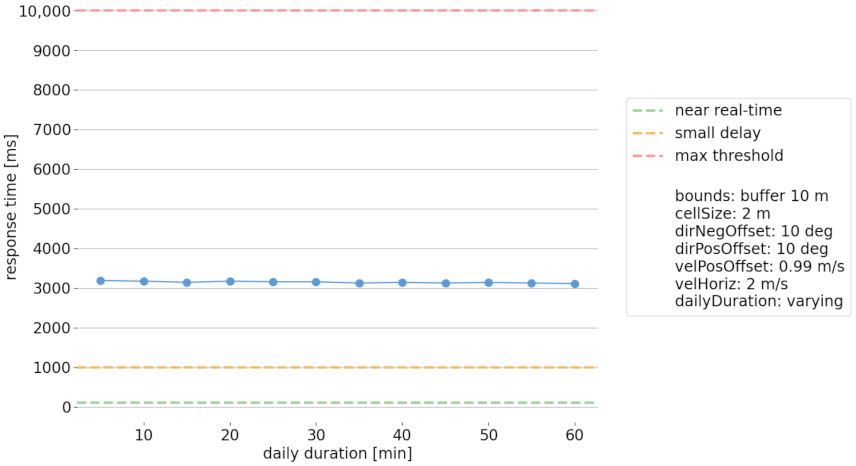
The direction_plan and duration_plan results showed that the wind direction offsets and the daily duration of the wind have insignificant impact in the response times in realistic scenarios, i.e., wind velocity above 2 m/s and a spatial buffer around the buildings of 10 m (Figure 17 and Figure 18).

The velocity_plan showed an exponential decay in the response time, while the horizontal velocity high-pass filter increased. This is an expected behavior in a city environment since blocking and occlusions by above surface objects decrease the wind velocity resulting in many locations with lower wind speeds. Despite the fact that there were cases above the 10,000 milliseconds threshold, the wind velocity was in the range of 1–1.3 m/s, which, in fact, is not a realistic scenario for a promising wind power yield (Figure 19).

7. Critical Review

In this study, an interactive visual analytics platform was presented that is able to locate areas in an urban environment where small scale wind turbines could be installed. The architecture is based on community best practices, and its implementation utilizes standardized web and 3D technologies. The visualization on the client side is based on a number of RESTful APIs. It is important to mention that the query parameter dailyDuration, of the query API, is a normalized value and does not guarantee the daily duration of the wind above the horizontal velocity threshold.

The performance of the platform was evaluated against the spatial domain volume, including various scenarios. Although the ground area of the domain volume reached over 2 km², the response time stayed below the limit of the 10 s. Still, there is room for improvement, by employing spatial indexing, among other spatial capabilities of the PostgreSQL database system. PostgreSQL spatial indexing depends on the PostGIS extension, a data-driven R-Tree [35] structure which uses the idea of a spatial containment relationship. Although spatial indexes aim for the query planning improvement, there are cases where this may result in efficiency degradation, which may adversely affect query performance. Counter-intuitively, it is not always faster to do an index search: if the search is going to return every record in the table, traversing the index tree to get each record will be slower than sequentially reading the whole table [36].

Partitioning the data regarding the CFD results will considerably decrease parts of the database queries where joins are performed, since the the first step of any database join is a Cartesian product. The linear performance of our workflow, while the query bounds increase is an indicator that it cannot scale and remain interactive. For this reason, a streaming design is favorable for achieving real-time results in our future work. Expanding the search domain in higher geographical and administrative regions would require the streaming of hierarchical 3D delivery formats, namely 3D-Tiles [37] and I3S [38], which are widely adopted OGC community standards.

The case study area reported in this paper (about 0.2 km²) is the urban quarter “Neuer Stöckach”, which belongs to the wider Stöckach area located in the center of Stuttgart. In this area, an energy concept is planned to integrate renewable energies. As part of the redevelopment/refurbishment, the integration of small wind turbines is considered. This case study has shown little potential for wind turbines investment for the reason that the topography of the area is not suitable. The study area is affected by the wake of hill located South-West about 6 km away. High wind velocities, above 4 m/s, were detected in areas about 100 m above residential houses, far exceeding the German regulations (10 m). In addition, the daily duration in the previously mentioned areas was in the range of 60 min, which is considered a prohibiting value for wind energy investment.

The client application, in beta version, can be accessed at http://hellowind.xyz (accessed on 11 October 2021). A wind yield calculation module is already implemented but not published yet.

References

1. Keim, D.; Kohlhammer, J.; Ellis, G.; Mansmann, F. (Eds.) Mastering the Information Age: Solving Problems with Visual Analytics; Eurographics Association: Goslar, Germany, 2010. [Google Scholar]
2. Blocken, B. Computational Fluid Dynamics for urban physics: Importance, scales, possibilities, limitations and ten tips and tricks towards accurate and reliable simulations. Build. Environ. 2015, 91, 219–245. [Google Scholar] [CrossRef] [Green Version]
3. Gröger, G.; Plümer, L. CityGML—Interoperable semantic 3D city models. ISPRS J. Photogramm. Remote Sens. 2012, 71, 12–33. [Google Scholar] [CrossRef]
4. Suomisto, J.; Airaksinen, E.; Bergstrom, M.; Heinonnen, H.; Lahti, K.; Kaisla, K. The Kalasatama Digital Twins Project; Technical Report, Helsinki 3D+; Helsinki Urban Environment Division: Helsinki, Finland, 2019. [Google Scholar]
5. Franke, J.; Baklanov, A. Best Practice Guideline for the CFD Simulation of Flows in the Urban Environment: COST Action 732 Quality Assurance and Improvement of Microscale Meteorological Models; Meteorological Institute, University of Hamburg: Hamburg, Germany, 2007. [Google Scholar]
6. Islam, M.; Mekhilef, S.; Saidur, R. Progress and recent trends of wind energy technology. Renew. Sustain. Energy Rev. 2013, 21, 456–468. [Google Scholar] [CrossRef]
7. Hand, B.; Cashman, A. Conceptual design of a large-scale floating offshore vertical axis wind turbine. Energy Procedia 2017, 142, 83–88. [Google Scholar] [CrossRef]
8. Borg, M.; Shires, A.; Collu, M. Offshore floating vertical axis wind turbines, dynamics modelling state of the art. part I: Aerodynamics. Renew. Sustain. Energy Rev. 2014, 39, 1214–1225. [Google Scholar] [CrossRef] [Green Version]
9. Balduzzi, F.; Bianchini, A.; Carnevale, E.A.; Ferrari, L.; Magnani, S. Feasibility analysis of a Darrieus vertical-axis wind turbine installation in the rooftop of a building. Appl. Energy 2012, 97, 921–929. [Google Scholar] [CrossRef]
10. Tabrizi, A.B.; Whale, J.; Lyons, T.; Urmee, T. Performance and safety of rooftop wind turbines: Use of CFD to gain insight into inflow conditions. Renew. Energy 2014, 67, 242–251. [Google Scholar] [CrossRef] [Green Version]
11. Mithraratne, N. Roof-top wind turbines for microgeneration in urban houses in New Zealand. Energy Build. 2009, 41, 1013–1018. [Google Scholar] [CrossRef]
12. Lee, K.Y.; Tsao, S.H.; Tzeng, C.W.; Lin, H.J. Influence of the vertical wind and wind direction on the power output of a small vertical-axis wind turbine installed on the rooftop of a building. Appl. Energy 2018, 209, 383–391. [Google Scholar] [CrossRef]
13. Ledo, L.; Kosasih, P.; Cooper, P. Roof mounting site analysis for micro-wind turbines. Renew. Energy 2011, 36, 1379–1391. [Google Scholar] [CrossRef]
14. Rezaeiha, A.; Montazeri, H.; Blocken, B. A framework for preliminary large-scale urban wind energy potential assessment: Roof-mounted wind turbines. Energy Convers. Manag. 2020, 214, 112770. [Google Scholar] [CrossRef]
15. Al-Quraan, A.; Stathopoulos, T.; Pillay, P. Comparison of wind tunnel and on site measurements for urban wind energy estimation of potential yield. J. Wind. Eng. Ind. Aerodyn. 2016, 158, 1–10. [Google Scholar] [CrossRef] [Green Version]
16. Hausdorff, F. Grundzuege der Mengenlehre; Chelsea: New York, NY, USA, 1965. [Google Scholar]
17. Beller, C. Urban Wind Energy. Ph.D. Thesis, Technical University of Denmark, National Laboratory for Sustainable Energy, Roskilde, Denmark, 2011. [Google Scholar]
18. Moeng, C.H.; Sullivan, P. Numerical Models|Large-Eddy Simulation. In Encyclopedia of Atmospheric Sciences, 2nd ed.; North, G.R., Pyle, J., Zhang, F., Eds.; Academic Press: Oxford, UK, 2015; pp. 232–240. [Google Scholar] [CrossRef]
19. Blocken, B. LES over RANS in building simulation for outdoor and indoor applications: A foregone conclusion? Build. Simul. 2018, 11, 1–50. [Google Scholar] [CrossRef] [Green Version]
20. Wang, B.; Sun, S.; Duan, M. Wind potential evaluation with urban morphology—A case study in Beijing. Energy Procedia 2018, 153, 62–67. [Google Scholar] [CrossRef]
21. Juan, Y.H.; Wen, C.Y.; Chen, W.Y.; Yang, A.S. Numerical assessments of wind power potential and installation arrangements in realistic highly urbanized areas. Renew. Sustain. Energy Rev. 2021, 135, 110165. [Google Scholar] [CrossRef]
22. Chtibi, A.; Touzani, A. Actual wind energy use situation worldwide and in Morocco: Case of small vertical axis wind turbine market offers. In Proceedings of the 4th International Conference on Big Data and Internet of Things, Tangier-Tetuan, Morocco, 23–24 October 2019; pp. 1–7. [Google Scholar] [CrossRef]
23. Wilkinson, S.; Bradbury, G.; Hanna, S. Approximating Urban Wind Interference. In Proceedings of the Symposium on Simulation for Architecture & Urban Design; Society for Computer Simulation International: San Diego, CA, USA, 2014. [Google Scholar]
24. Ágota Szűcs. Wind comfort in a public urban space—Case study within Dublin Docklands. Front. Archit. Res. 2013, 2, 50–66. [Google Scholar] [CrossRef] [Green Version]
25. Keim, D.A.; Bak, P.; Bertini, E.; Oelke, D.; Spretke, D.; Ziegler, H. Advanced Visual Analytics Interfaces. In Proceedings of the International Conference on Advanced Visual Interfaces; Association for Computing Machinery: New York, NY, USA, 2010; pp. 3–10. [Google Scholar] [CrossRef] [Green Version]
26. Cybulski, J.; Keller, S.; Saundage, D. Metaphors in Interactive Visual Analytics. In Proceedings of the 7th International Symposium on Visual Information Communication and Interaction; Association for Computing Machinery: New York, NY, USA, 2014; pp. 212–215. [Google Scholar] [CrossRef]
27. Ferreira, N.; Lage, M.; Doraiswamy, H.; Vo, H.T.; Wilson, L.; Werner, H.; Park, M.; Silva, C.T. Urbane: A 3D framework to support data driven decision making in urban development. In Proceedings of the 2015 IEEE Conference on Visual Analytics Science and Technology (VAST), Chicago, IL, USA, 25–30 October 2015; Curran Associates: New York, NY, USA; pp. 97–104. [Google Scholar]
28. Deininger, M.E.; von der Grün, M.; Piepereit, R.; Schneider, S.; Santhanavanich, T.; Coors, V.; Voß, U. A Continuous, Semi-Automated Workflow: From 3D City Models with Geometric Optimization and CFD Simulations to Visualization of Wind in an Urban Environment. ISPRS Int. J. Geo-Inf. 2020, 9, 657. [Google Scholar] [CrossRef]
29. Gaillard, J.; Vienne, A.; Baume, R.; Pedrinis, F.; Peytavie, A.; Gesquière, G. Urban Data Visualisation in a Web Browser. In Proceedings of the 20th International Conference on 3D Web Technology; Association for Computing Machinery: New York, NY, USA, 2015; pp. 81–88. [Google Scholar] [CrossRef] [Green Version]
30. Patterson, D. Interactive 3D Web Applications for Visualization of World Health Organization Data. In Proceedings of the Australasian Computer Science Week Multiconference; Association for Computing Machinery: New York, NY, USA, 2016. [Google Scholar] [CrossRef]
31. Schilling, A.; Bolling, J.; Nagel, C. Using GlTF for Streaming CityGML 3D City Models. In Proceedings of the 21st International Conference on Web3D Technology; Association for Computing Machinery: New York, NY, USA, 2016; pp. 109–116. [Google Scholar] [CrossRef]
32. Handsaker, S.; Ogbonna, I.; Volkov, K. CFD Prediction of Performance of Wind Turbines Integrated in the Existing Civil Infrastructure. Sustainability 2021, 13, 8514. [Google Scholar] [CrossRef]
33. Stadtklima-stuttgart.de. Download von Messdaten der Station S-Mitte, Schwabenzentrum. 2020. Available online: https://www.stadtklima-stuttgart.de/index.php?luft_messdaten_download (accessed on 8 June 2021).
34. Hagedorn, B.; Thum, S.; Reitz, T.; Coors, V.; Gutbell, R. 3D Portrayal Service Version 1.0. 2017. Available online: http://docs.opengeospatial.org/is/15-001r4/15-001r4.html (accessed on 25 August 2021).
35. Guttman, A. R-Trees: A Dynamic Index Structure for Spatial Searching. In Proceedings of the 1984 ACM SIGMOD International Conference on Management of Data; Association for Computing Machinery: New York, NY, USA, 1984; pp. 47–57. [Google Scholar] [CrossRef]
36. Ramsey, P. Spatial Indexing—Introduction to PostGIS. 2021. Available online: https://postgis.net/workshops/postgis-intro/indexing.html (accessed on 27 August 2021).
37. Cozzi, P.; Lilley, S.; Getz, G. 3D Tiles Specification. 2018. Available online: https://github.com/CesiumGS/3d-tiles/tree/master/specification (accessed on 26 August 2021).
38. ESRI. I3S Specification. 2019. Available online: https://github.com/Esri/i3s-spec (accessed on 26 August 2021).
Figure 1. Visualization of CFD simulation attributes to indicate/exclude locations for/from further investigation. (Left) Color encoded locations in red hue indicate high turbulence areas which should be excluded from further analysis. Color encoded locations in yellow hue indicate areas of high wind pressure on building façades, and further analysis is recommended. (Right) Color encoded locations in purple hue indicate areas with high wind pressure on buildings near eaves height.
Ijgi 10 00707 g001
Figure 2. An array of three wind turbines is integrated between the two towers of the Bahrain World Trade Center (by Denise Krebs is licensed with CC BY 2.0. To view a copy of this license, visit https://creativecommons.org/licenses/by/2.0/ (accessed on 11 October 2021)).
Ijgi 10 00707 g002
Figure 3. Conceptual graph of the workflow.
Ijgi 10 00707 g003
Figure 4. A 3D feature grid with three historical events in a cell. The dots represent the locations of the velocity vectors. The red and yellow vector are results of the same CFD simulation since they are produced from the same wind direction (assuming the same wind speed in the historical data).
Ijgi 10 00707 g004
Figure 5. The integration of historical wind data and CFD wind fields will generate a three-dimensional grid. Each grid cell will enclose useful spatial, attributive, and temporal information for decision-making strategies.
Ijgi 10 00707 g005
Figure 6. From left to right: The data tier, application tier, and web tier of the full-stack application.
Ijgi 10 00707 g006
Figure 7. Annual wind direction and wind speed (for SW direction) probabilities for the years 2017–2019 in the Stöckach area.
Ijgi 10 00707 g007
Figure 8. Overview of the implementation: The server side is comprised of a PostgreSQL database to host the CFD and historical data. Both services, 3DPS and Query API, are implemented in Node.js. 3DPS implementation allows dynamic 3D assets fetching hosted in a relational database and static 3D assets stored in the file-system.
Ijgi 10 00707 g008
Figure 9. The public PostgreSQL database schema. In snake case are the column names and in capital the data types and additional directives.
Ijgi 10 00707 g009
Figure 10. The process flow of the spatio-temporal grid generation.
Ijgi 10 00707 g010
Figure 11. Definition of an ROI in area mode.
Ijgi 10 00707 g011
Figure 12. The web client user interface. Definition of four Regions of Interest in the case study area of Stöckach, Stuttgart. ROI from left to right: (ROI584) Spatio-temporal layer displaying locations of horizontal wind velocity above 3 m/s and daily duration above 30 min. (ROI12) Spatio-temporal layer displaying locations of horizontal wind velocity above 1.5 m/s and daily duration above 30 min. (ROI569) Spatial layer displaying pressure using point primitive. (ROI560) Spatial layer displaying velocity using vector primitive.
Ijgi 10 00707 g012
Figure 13. From top to bottom: The layer editor wizard, the layer settings for a spatial layer, and the layer settings for a spatio-temporal layer.
Ijgi 10 00707 g013
Figure 14. The visual analytics platform remained interactive even in larger spatial extents.
Ijgi 10 00707 g014
Figure 15. The response times when the grid cell varies.
Ijgi 10 00707 g015
Figure 16. The response times and the grid size when the grid cell varies.
Ijgi 10 00707 g016
Figure 17. The response times when the wind direction offset varies.
Ijgi 10 00707 g017
Figure 18. The response times when the wind daily duration varies.
Ijgi 10 00707 g018
Figure 19. The response times when the horizontal velocity high-pass filter varies.
Ijgi 10 00707 g019