Fully Automated Pose Estimation of Historical Images in the Context of 4D Geographic Information Systems Utilizing Machine Learning Methods

Abstract

The idea of virtual time machines in digital environments like hand-held virtual reality or four-dimensional (4D) geographic information systems requires an accurate positioning and orientation of urban historical images. The browsing of large repositories to retrieve historical images and their subsequent precise pose estimation is still a manual and time-consuming process in the field of Cultural Heritage. This contribution presents an end-to-end pipeline from finding relevant images with utilization of content-based image retrieval to photogrammetric pose estimation of large historical terrestrial image datasets. Image retrieval as well as pose estimation are challenging tasks and are subjects of current research. Thereby, research has a strong focus on contemporary images but the methods are not considered for a use on historical image material. The first part of the pipeline comprises the precise selection of many relevant historical images based on a few example images (so called query images) by using content-based image retrieval. Therefore, two different retrieval approaches based on convolutional neural networks (CNN) are tested, evaluated, and compared with conventional metadata search in repositories. Results show that image retrieval approaches outperform the metadata search and are a valuable strategy for finding images of interest. The second part of the pipeline uses techniques of photogrammetry to derive the camera position and orientation of the historical images identified by the image retrieval. Multiple feature matching methods are used on four different datasets, the scene is reconstructed in the Structure-from-Motion software COLMAP, and all experiments are evaluated on a newly generated historical benchmark dataset. A large number of oriented images, as well as low error measures for most of the datasets, show that the workflow can be successfully applied. Finally, the combination of a CNN-based image retrieval and the feature matching methods SuperGlue and DISK show very promising results to realize a fully automated workflow. Such an automated workflow of selection and pose estimation of historical terrestrial images enables the creation of large-scale 4D models.

1. Introduction

The idea of virtual time machines in digital environments like hand-held virtual reality (VR) or four-dimensional (4D) geographic information systems (GIS) requires an accurate positioning and orientation (=pose) of historical images. This enables texturing three-dimensional (3D) models (see Figure 1) and offers new perspectives of spatial distributions of historical data [1] as these photographs are sometimes the only visual remainder of buildings due to renovation or destruction of the respective object. The range of historical image data over time represents the fourth dimension as a temporal component, allowing the user to travel through space and time, and thus, makes cultural heritage tangible.

With the ongoing mass-digitization in archives and libraries, an increasing amount of image data became available to the public. Nowadays, the quality aspects of image data such as a higher resolution and lossless data formats, allow the use of automatic image analysis on historical image data. However, often the repositories show varying metadata and usability quality [2,3], and thus, the usage of historical data material for a photogrammetric reconstruction of buildings and structures relies heavily on archive browsing and manually selecting appropriate sources [4,5,6,7]. This contribution tackles this problem focusing on a completely automated retrieval and pose estimation workflow for historical terrestrial images using deep learning methods.

The starting point is getting images of interest from an image database or repository. This step can be automated by using content-based image retrieval, whereby retrieval methods based on convolutional neural networks are used. Our approach provides the option to crawl an image database using multiple (in our experiments three) query images containing the object of interest. As metadata in databases and repositories is often inconsistent, misleading, or incorrect, it makes sense not to rely only on a metadata search and to apply image retrieval.

The retrieval result is directly used as input for an automatic six degrees-of-freedom (6-DoF) pose estimation workflow, i.e., calculation of the camera position and camera orientation up to scale. Especially the automatic detection of distinctive features and their matching are the most difficult tasks when calculating the image pose [8]. This is because the images were mostly made by different people at different times in no photogrammetric context, e.g., a convergent image block with significant overlap between the images. Additionally, large baselines, occlusions, environmental changes, and scale differences hamper the feature matching process. Thus, more advanced methods which are possibly able to deal with these difficulties are tested and evaluated.

However, for the evaluation of feature matching methods, no or only small datasets consisting of exclusively historical images are available. This contribution tries to overcome this issue, by creating and publishing four datasets with a mimimum of 20 images with manually determined feature points suitable for a Structure-from-Motion (SfM) workflow http://0-dx-doi-org.brum.beds.ac.uk/10.25532/OPARA-146, accessed on 3 November 2021. This benchmark data allows an evaluation of the performance of five different feature matching methods, all relying on deep neural networks.

In the second evaluation, all the methods are once again used to process the larger datasets derived by the preceding image retrieval. This workflow shown in Figure 2 and explained in detail in Section 4, enables the calculation of the orientation parameters of a large percentage of the historical images by only selecting three query images. The estimated poses can be transferred to different browser applications.

2. Related Work

This section intends to give a (nonexhaustive) overview of methods for image retrieval and feature matching in the photogrammetric context of calculating the camera position and orientation of historical images. For a summary of 3D building reconstruction approaches based on the works of [9,10] using historical images refer to [8].

2.1. Image Retrieval

Content-based image retrieval (AKA content-based instance retrieval) is a classical task that computer vision is dealing with during the last decades already (e.g., cf. [11]). Thereby, it turned out to be a challenging task and was tackled with many different approaches. Image retrieval approaches based on deep neural networks show good or at least promising performance in comparison to former standard approaches as, e.g., VLAD, Bag-of-Words or improved Fisher vectors (cf. ([12], Section 4, Table 7), or ref. [13]). A good overview on the development of further more recent retrieval methods can be found in [14]. The approach of (p. 255, [15]) that is based on a convolutional neural network (CNN) even outperformed the common image representations as VLAD and IFV. Using a CNN for this task is plausible as such a network is able to catch the characteristics of an image, e.g., edges, shapes, lines within so-called feature maps (cf. [16]). These feature maps can be used as descriptors of an image. By decomposing an image into several subimages, there are created multiple local descriptors as proposed in [15]. In [17,18] the retrieval approach of [15] was already successfully applied to heterogeneous historical images and it showed promising results to identify images that contain some given object of interest.

One approach to improve the usage of local descriptors is called attentive deep local features (DELF), cf. [19]. Therein, the relevance of single local descriptors is learned by a second neural network. Furthermore, potential matches are geometrically verified with the RANSAC algorithm, cf. [20]. For image retrieval, the article at hand is intended to compare the approaches of [15,19] and to investigate their utilization for finding relevant images for purposes of photogrammetry. To the best of our knowledge content-based image retrieval has not yet been applied exclusively to historical images within photogrammetry.

2.2. Feature Detection and Matching

While there is little research focusing on the evaluation of feature matching methods using exclusively historical images [8] a lot of methods are tested on difficult benchmark datasets, e.g., the Photo Tourism dataset [21] and the Aachen Day-Night dataset [22]. With an increasing use of neural networks for feature detection, matching, and scene reconstruction an overview of well-performing, recently published methods using diverse network architectures is given in this section.

Several studies show that the commonly used algorithmic (“handcrafted”) method SIFT [23] in combination with advanced matching methods is still able to perform comparable to deep local invariant features [24,25,26,27]. Thus, the training of a neural network for an end-to-end pipeline from feature detection to feature description up to feature matching seems like a promising approach. Other approaches even go further and include the final camera pose in the network architecture [28]. The network should get an understanding what makes a good feature, how to describe it distinctively, how to combine multiple matches to generate a robust matching solution, and how to estimate a reasonable and accurate pose.

A lot of different approaches using deep neural networks were already developed in the past. Some of them learn optimized descriptors [29,30,31,32], others combine the descriptor learning with a metric learning approach to include the feature matching into the network [33,34].

As a further improvement, multiple recent methods focus on the joint detection and description of features in a single network architecture [35,36,37]. A focus lies especially on the methods D2-net [38] and R2D2 [39], which are used in the photogrammetric workflow and evaluation (see Section 4) of this contribution.

D2-Net is a winner of the Image Matching Challenge of the IEEE Conference on Computer Vision and Pattern Recognition (CVPR 2019) and already produced good results in recent research on historical images [8]. The method jointly detects and describes stable feature matches using a CNN which extracts a set of feature maps for every single image. A local descriptor is obtained by traversing all feature maps at a spatial position in the image while the keypoint detections are obtained by performing a non-local-maximum suppression on a feature map followed by a non-maximum suppression across each descriptor [38].

To train the network, D2-Net uses a loss function jointly optimizing the detection and description objectives by minimizing the distance of corresponding descriptors while maximizing the distance to other distracting descriptors.

R2D2 follows a similar approach to D2-net and jointly detects and describes keypoints by training a fully-convolutional network. The method achieved superior results compared to D2-net on benchmark datasets [27]. R2D2 uses a slightly modified L2-Net [31] as a backbone and adds two different layer structures to obtain a respective map for repeatability and reliability [39]. This allows separate learning and optimizing of repeatability and reliability for the matching process. Still, both methods rely on a feature matching strategy using Lowe’s ratio test.

As final and most recent approaches, end-to-end pipelines (including detection, description and matching) are compared, especially SuperGlue [40] and DISK [41]. For the new promising approach Pixloc [28], which also integrates the 6-DoF-Pose into the neural network to learn the feature, the code was just recently published and could not be tested yet. In the strict sense, SuperGlue is only a feature matching method, however, the authors combine it in a complete pipeline using the SuperPoint feature detector [32]. The pipeline is a winner of the CVPR Image Matching Challenge 2020. SuperPoint uses a modified VGG16 network [42] as encoder and add two different decoders for keypoint detection as well as description.

Firstly, this feature detector is pretrained on synthetic data and is referred to as MagicPoint. Secondly, the geometric consistency of MagicPoint is improved using Homographic Adaption. This process is self-supervised and allows an iterative repetition. The resulting model is called SuperPoint and is used for the feature detection in the SuperGlue workflow.

SuperGlue introduces a novel method for the matching of the derived features using a graph neural network to solve a differentiable optimal transport problem where relevant information is directly learned from the data. SuperGlue uses two major components. An attentional graph neural network is used with a keypoint encoder to map feature positions and their descriptors into a single vector. Then, more powerful representations are generated in self- and cross attention layers. In the second component, an optimal matching layer finds the optimal partial assignment using the Sinkhorn algorithm [40].

DISK is a complete pipeline for extracting, describing and matching image features. The process of feature extraction is based on a modified U-net architecture [43] while optimizing the absolute number of feature matches using Reinforcement Learning with positive and negative rewards for correct and incorrect matches, respectively. Therefore, gradients of expected rewards are estimated using Monte Carlo sampling and the gradient ascent is used for maximizing the quantity of obtained feature matches.

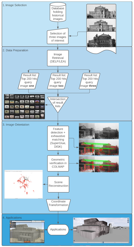
3. Data Preparation: Image Retrieval

This section of the article deals with the image retrieval process for getting images of interest that are processed later by methods of photogrammetry. Thereby, the idea is extended by looking in particular at experimental settings that correspond to the real situation a researcher in photogrammetry faces when searching for images that contain the object of interest (OoI). More specifically, it is investigated to which extent an image retrieval approach is suitable for refining search results from a metadata search, replacing the manual process of filtering hundreds or even thousands of images. Two CNN-based retrieval approaches are considered: (1) the approach according to [15], that will be called layer extraction approach (LEA) in the following, (2) the approach according to [19], which is the DELF approach. For every image retrieval there are two types of images: (a) the query image with the OoI, (b) the reference images that are to be compared.

Both approaches were implemented from scratch based on the corresponding publications. The implementations were realized in Python 3.8 with Pytorch 1.7. All experiments were performed on Nvidia A100 GPUs.

3.1. Experiment and Data

The experiments are intended to compare the performance between metadata (MD) search and image retrieval (IR). Thereby, the basic idea is to use the MD search as a kind of prefiltering and, in a second step, to improve the result quality by applying an IR to the MD search results. The concrete procedure of the experiment is as follows:

1.

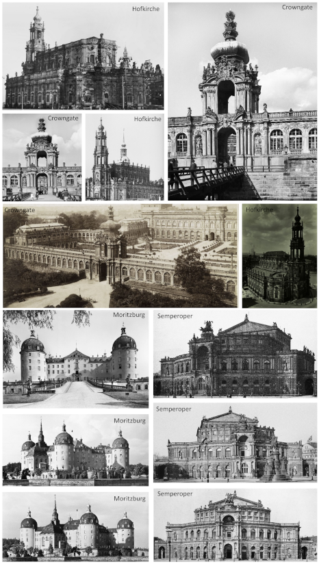
A fixed number of OoI in the vicinity of Dresden, Germany is defined: Frauenkirche, Hofkirche, Moritzburg, Semperoper, Sophienkirche, Stallhof, Crowngate

2.

For each OoI, a MD search is performed returning a list of results. Note that each of these result lists contains a different number of images across the different OoI.

3.

The result list from step 2. is sorted by two criteria: by name and recording date (ascending and descending each). As an outcome, there is a total of four result lists from the MD search for every single OoI.

4.

To perform IR, for each OoI three query images are defined. Based on each query image, both IR approaches (LEA, DELF) are applied to the result list of every OoI from step 2. The outcome here is one result list per query image with the most similar images at the top.

5.

All result lists from step 3. and step 4. are evaluated for the top-200 positions (more details on evaluation in Section 3.3).

The MD search was conducted via the Saxon State and University Library Dresden (SLUB) using the browser-based search interface in Deutsche Fotothek and resulted in a total of 4737 images. These image data cover a time range from about 1850–2005 and contain historic photographs and a few drawings. Examples of the images are shown in Figure 3 in the photogrammetry section. All found images were annotated manually whether they match the defined OoI or not. These chosen OoI are seven different sights in the vicinity of Dresden. As some buildings are located very close to each other in the inner city, several OoI may appear simultaneously on one image. Thus, some images are assigned to multiple OoI.

The data contain different file formats (jpg, tif, gif) and color spaces, as well as varying resolutions, with smallest images of size $257\times 400$ and largest of size $3547\times 2847$. During a preprocessing step all images were converted into jpg-format with RGB color channels without changing the resolution.

3.2. Methods

This section sketches the two IR approaches used within the experiments. Both are based on a CNN. More precisely, LEA is based on VGG-16 and DELF is based on Resnet50. The basic idea is similar for both: single network layers are used as a numerical representation of a single image for comparing and assessing the distance between many images. Using CNNs for that task seems plausible, as this type of neural networks is able to catch the main characteristics of an image, like edges, shapes, lines, etc.

For the sake of simplicity, the following method descriptions are mainly intended to convey the basic idea of an approach as well as the relevant parameters and their impact on the application. For further details we refer to the corresponding publications.

3.2.1. Layer Extraction Approach (LEA)

The IR was implemented according to [15]. This approach is based on a pretrained CNN (here: VGG-16 from [42]), where one of the upper layers (here: the last max-pooling layer) is used as a vector-based image representation for each image. The output of the last max-pooling layer is 512 so-called feature maps, each with dimension $7\times 7$. According to (p. 253, [15]), these feature maps are reduced in dimension by using spatial pooling (aka global max-pooling). This standard operation of max-pooling (cf. (Section 5.1.2, [44])) can be performed using different parameters, mainly kernel size and stride. The resulting set of feature maps is flattened to a vector whose length depends on the parameters used. Within the experiments, two different parameter settings for max-pooling are used:

1.

kernel size $7\times 7$ with stride 0, leading to resulting feature maps of size $1\times 1$ each (i.e., maximum reduction); flattened to vector of size $512\times 1\times 1=512$

2.

kernel size $4\times 4$ with stride 3, leading to resulting feature maps of size $2\times 2$ each; flattened to vector of size $512\times 2\times 2=2048$

The resulting vector representations within each setting have the same size for each image and are used to calculate a distance measure between the query image and each reference image. Here, the Euclidean distance is used. Within a last step, an ordered rank-list is created based on the distances calculated.

The result of a single IR based on one query image is a sorted list (rank-list) of images, containing the distance between the query image and each reference image, with best matches on top.

To improve the retrieval results, the query images and the reference images are divided into subpatches (part of image by cropping) according to (p. 254, Equations (1) and (2), [15]). The level of division is characterized by the order parameter L. The number of resulting subpatches is determined by ${\sum }_{i=1}^L{i}^2$, e.g., an order of $L=4$ leads to 30 subpatches. Within the experiments in [15] an order of $L=3$ and $L=4$ led to good results.

For the application at hand, we use a fixed query order of 3, i.e., 14 sub-patches for the query images. The number of subpatches of reference images, denoted as reference order, is varied for $L=3$ and $L=4$ within different experiment settings. Using subpatches of query and/or reference images, the above procedure of distance calculation is applied for every single pair of subpatches. Thereby, these distances need to be aggregated into one final distance number, which is done here following (p. 255, Equations (3) and (4), [15]). The chosen parameters (query order, reference order, max-pooling) for LEA are motivated from [15] and, especially for heterogeneous historical images, from [18].

Moreover, in (p. 256, [15]) all images were resized to 600 × 600 pixels as preprocessing step and this size turned out to provide the best retrieval results based on the datasets used there. In contrast, we found that the retrieval results are quite robust against resizing and that there is no relevant change in the retrieval results. Furthermore, in (p. 255, [15]) a principal component analysis (PCA) and whitening is used after the max-pooling to further reduce the dimension of the vector representations. This kind of postprocessing turned out to be beneficial for the retrieval quality, cp. (p. 255, Table 1, [15]) or cf. [45]. Nevertheless, we could not observe any relevant change or even structural improvement of retrieval results while using such kind of postprocessing. One reason for this could be that, unlike [15,45], we do not use fixed benchmark datasets, but real data that potentially varies widely across retrievals. Overall, for sake of simplicity we do not report the retrieval results from resizing and PCA.

3.2.2. Attentive Deep Local Features (DELF) Approach

The approach in this section is based on an attentive local feature descriptor and is referred to as DELF (DEep Local Feature) [19]. The DELF IR pipeline consists of four steps: (1) dense localized feature extraction; (2) feature selection; (3) dimensionality reduction; (4) indexing and retrieval.

In the first step, the dense features are extracted by using the convolutional neural network ResNet50 [46], trained on ImageNet [47] as a baseline. As in the original paper, the weights of the ResNet50 neural network are fine-tuned on the annotated dataset of landmark images (Google Landmark Challenge V2 [48]), to achieve better discriminative power of the descriptors for the landmark retrieval problem. The output of the forth convolutional layer is used to obtain feature maps.

In the second step, to select a subset of relevant features from dense feature maps an attention-based selection technique is used. Therefore, a different neural network (attention network) is trained from scratch (again on Google Landmark Challenge V2), to learn which feature maps are relevant. This restriction to relevant features helps to improve accuracy and to increase computational efficiency. For more details the reader is referred to the original paper, ref. [19].

The selected feature maps with 1000 features per image, each of size 1024, are still too large to run efficient comparisons. Therefore, similarly as in the original paper, dimensionality reduction with PCA is applied. After normalization, the feature vectors of up to 500 images are collected and $k\in \{40,120,200\}$ principal components are calculated for the reference dataset.

In the last step, the actual matching of the query image to each image in the reference dataset is realized. The reference images are sorted according to the similarity to the query image. The Euclidian distance between the pairs of feature vectors is calculated and compared to a distance threshold $T\in \{1.0,1.2,1.4\}$. If the distance remains below the threshold, it is noted as a potential match and is discarded otherwise. Subsequently, potential matches are geometrically verified. If the images contain the same OoI, there exists an affine transformation, which transforms the positions of the features on the query image to those on the reference image. The RANSAC algorithm (RANdom SAmple Consensus) [20] is used for geometric verification. The number of verified matches is used as a measure of similarity, so-called score.

The distance threshold T has substantial impact on the retrieval results and should be chosen very carefully. Too large values of T lead to many false matches of feature maps within the considered image pair, while too small values provide no matches at all. To simplify the choice of the threshold, the distribution of scores can be evaluated by means of, e.g., a histogram. Ideally, the distribution should not be highly skewed to the left or right. For the application, here we found (using the histogram) $T=1.2$ to deliver good results.

Another parameter, the number of principal components k, has less influence on the retrieval quality than the distance threshold. Here, we could find a good compromise between accuracy (large k) and computational performance of the retrieval (small k). The evaluation of retrieval results for different values of k are presented in Figure 4. Thus, we extend the investigation from [19] who used the parameters for PCA $k=40$ and distance threshold $T=0.8$ and no other parameter settings were considered.

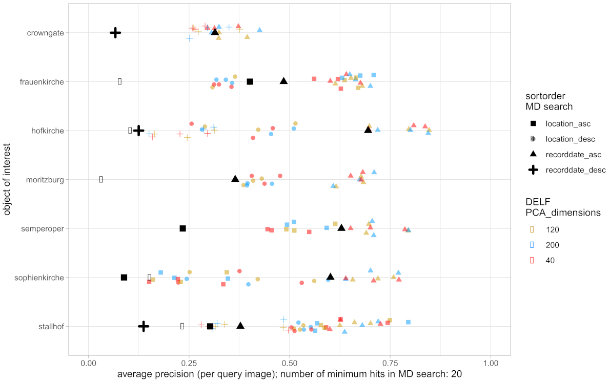
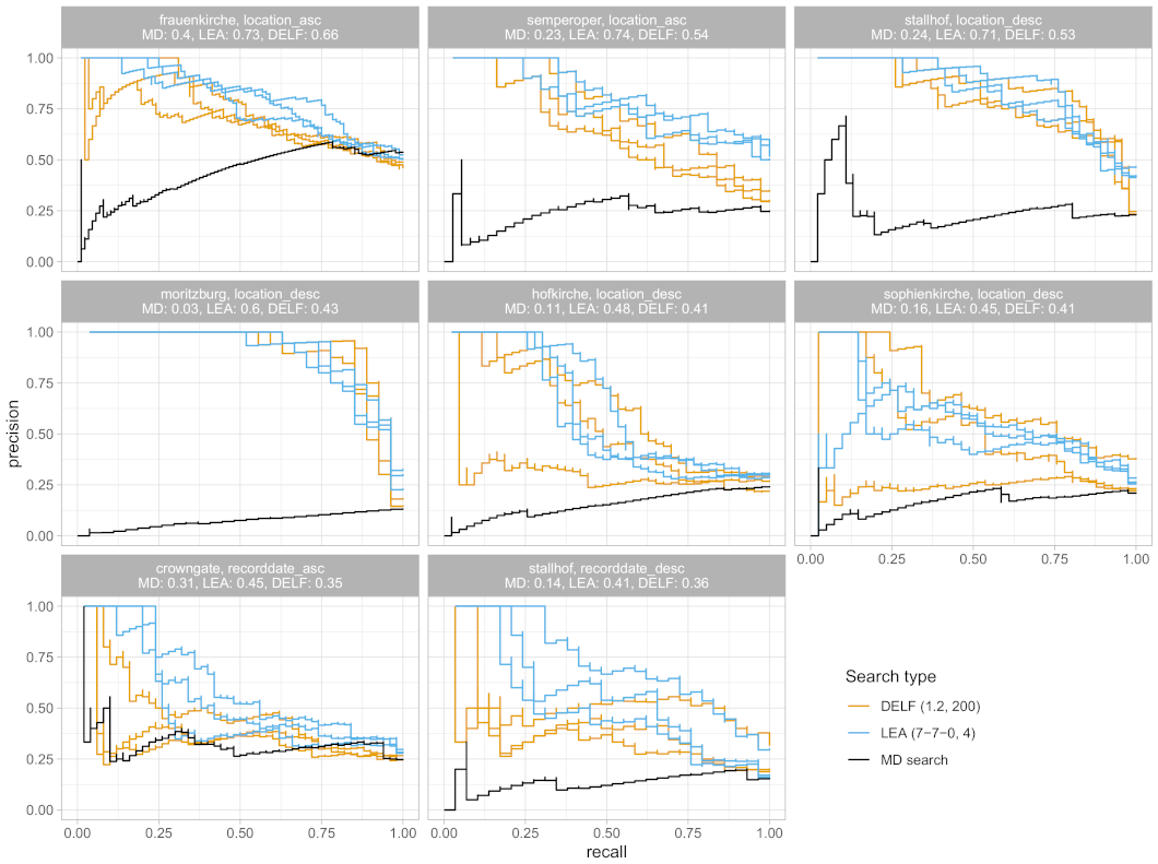
3.3. Results and Evaluation

The following results are based on the experimental setting described above in Section 3.1. More specifically, each metadata (MD) search result for the 7 objects of interest (OoI) considered can be sorted by recording date and location, in ascending and descending order, respectively. This leads to 28 result lists over all 7 OoI for the MD search. For each result list from the MD search an image retrieval (IR) is performed for improving the order of the list. These image retrievals are based on 3 different query images for every OoI, leading to 3 (potentially improved) result lists. Eventually, there are 7 OoI, 4 sorting criteria for MD search and 3 query images per OoI—leading to a total of $7\times 4\times 3=84$ result lists for each of the two approaches (LEA and DELF). As already described above, LEA and DELF can be configured by choosing different parameters like reference order, max-pooling parameters (for LEA) or distance threshold, PCA dimensions (for DELF). Within the experiments at hand, 3 different configurations for LEA and DELF were investigated. In total, this leads to $84\times 3\times 2=504$ result lists.

A single result list is a rank-list based on the top-200 images from the MD search. The sorting criteria are differing according to the applied method as follows:

• MD search: sorted by recording date and location, in ascending and descending order, respectively
• LEA, DELF: sorted by distance measure depending on the approach (top ranked positions have small distances to query image)

Based on the image annotation, every image can be categorized as “hit” or “miss” referring the OoI. A resulting ordered rank-list can be evaluated for each position on the list:

• relevant image before or at the considered position is a true positive (TP or a hit)
• irrelevant image that occurs before or at the considered position is a false positive (FP or a miss)

For evaluating these result lists, so-called precision-recall (PR) curves are used. Thereby, precision is defined as (cf. [49]) $precision=\frac{TP}{TP+FP}$. Recall is the fraction of collected hits w.r.t. to the total of possible hits. For every single position of the rank-list, precision and recall are calculated. Together they constitute a point on the PR curve (recall on x-axis; precision on y-axis). The perfect PR curve is a horizontal line at one, that describes a situation where all hits are directly one after another. More practically, a good PR curve tends to the upper-right corner. Note, that a result list is cut after the last possible hit, i.e., the last position always is a hit and all possible hits are collected therewith (i.e., recall equals one). Such a single PR curve is aggregated into one number by averaging the precision values along the curve, that leads to average precision (AP) ranging in the unit interval $[0,1]$.

Figure 5 shows a selection of PR curves for both, MD search and IR (LEA and DELF) over all three queries for the seven different OoI. The selection of these curves is intended to provide a coarse overview of the range of quality of the search results.

The interpretation for OoI “Frauenkirche” (Figure 5, top-left), for example, could be as follows. Finding roughly 50% (recall) of the OoI Frauenkirche means that approximately 70–90% (precision) of all images found to this point in the IR result list (blue and yellow curves) belong to OoI Frauenkirche. On the other hand, the precision of the MD search (black curve) for Frauenkirche is only 50%. From Figure 5, IR is leading to an improvement of MD search, i.e., the colored PR curves from IR (LEA, blue; DELF, orange) are substantially above the PR curve from the MD search in black. Furthermore, there is a slight difference in quality between the two IR approaches, LEA and DELF. This is indicated by the mean average precision (mAP). The mAP is an aggregation of multiple PR curves by calculating the mean over their single AP. The values in each subfigure refer to AP for MD search and mAP for LEA and DELF aggregating the corresponding PR curves. In Figure 5, the mAP is calculated separately for LEA and DELF, which shows slightly higher values for LEA.

To get the overall picture, Figure 4 and Figure 6 contain the AP values of IR while considering different parameter settings (max-pooling and reference order for LEA; PCA dimensions for DELF). The data shown in Figure 4 and Figure 6 refer to result lists that contain at least 20 hits for the OoI after MD search. This number of hits is regarded as a critical level due to practical considerations as this number of images is usually necessary to achieve enough redundancy for the SfM workflow.

To understand these figures, the following hints are essential:

• Basically, Figure 4 and Figure 6 are to be read line by line for the different OoI.
• For each OoI, the AP of the MD search is marked with a large black symbol (square, circle, etc.) as a reference value.
• The 4 different symbol shapes (square, circle, triangle, cross) refer to the considered sorting order for the MD search.
• Within each OoI there might be less than 4 symbol shapes due to the requirement of at least 20 hits from the MD search.
• Besides the black symbols, the other colors refer to different parameter settings of the IR approach under consideration. Since the IR is based on 3 query images, there are 3 symbols of the same shape and color within each line for each IR setting.
• Finally, symbols of the same shape belong together within each line, but can be compared across the lines for comparing different OoI as well.

In the following relevant observations that hold for both image retrieval approaches, LEA and DELF are listed.

1.

Most sorting criteria for MD search provide poor result lists with AP below 30%. This magnitude quantifies the trouble of practitioners (see Section 1) while searching images of relevance in databases and repositories.

2.

There are differences across the OoI referring to the IR quality and its deviation. Thereby, LEA performs slightly better and with less deviation than DELF.

3.

IR improves the quality of every MD search result list. More precisely, the improvement factor ($A{P}_{\mathrm{LEA}}/A{P}_{\mathrm{MD}}$) for LEA is around $2.6$ in 50% of the cases (factor $3.2$, 75% of the cases). The improvement factor ($A{P}_{\mathrm{DELF}}/A{P}_{\mathrm{MD}}$) for the DELF approach is around $1.9$ in 50% of the cases (factor $2.7$, 75% of the cases).

4.

Within the parameter settings illustrated there is no clear dependency on IR quality, i.e., no setting is preferred.

In summary, the results for AP are worse than those in [15] or [19]. Probably, this is caused by using different underlying data: the application at hand deals with a real dataset, that comes along with great heterogeneity in color, resolution, and image type, whereas benchmark datasets were used in [15,19]. In that sense, the data situation here is a realistic one and it provides insights about what is possible under real-world conditions. Nevertheless, the absolute values for mAP in the experiments at hand are still in the middle lower range of values for the quality of different IR approaches for the Oxford5k dataset (approx. 50–80%) as reported in (p. 1236, [14]). Generally, from the practitioner’s perspective an IR (no matter if LEA or DELF) substantially outperforms the MD search and can provide strong support for identifying images of interest.

4. Camera Pose Estimation of Historical Images Using Photogrammetric Methods

The main idea of this contribution is to use the output of the IR as a input for the pose estimation workflow. Usually, the simultaneous determination of 6-DoF pose and 3D object points for contemporary images is realized in conventional SfM software like e.g. Agisoft Metashape (proprietary) or Meshroom (open-source). However, these solutions often fail to orient historical images [17] due to their heterogeneous radiometric and geometric properties. Neural networks allow a more distinctive detection, description, and matching of features by training on thousands of ground truth image pairs. While these feature points and matches cannot yet be imported into the software solutions above, the presented method uses COLMAP [50] to process the feature matches derived by several neural networks to reconstruct a scene including camera positions, orientations and a sparse point cloud. COLMAP is the standard tool for benchmark tests and evaluations of the Image Matching Challenge of the IEEE Conference on Computer Vision and Pattern Recognition. Additionally, a benchmark dataset is generated and described to evaluate the results of the five different tested feature matching methods. All methods are also applied to larger datasets, which are directly derived by the image retrieval approach LEA (see Section 3.2.1) to bypass the process of manual image selection. The accuracy of the reconstruction and the total number of registered images can then again be verified by the benchmark dataset.

4.1. Data

For the evaluation of the automatic pose estimation workflow, two different lists (benchmark and retrieval) of respectively four datasets are created. The four datasets consist of historical terrestrial images in the vicinity of Dresden and all images originate from the Saxon State and University Library Dresden (SLUB). The analogue images are digitized by the the Deutsche Fotothek and can be downloaded in .jpg file format usually with a maximum edge length of 1600 pixels via http://www.deutschefotothek.de/, accessed on 20 September 2021. To compare the results to previous research, four different landmarks (Crowngate, Hofkirche, Moritzburg, Semperoper) are chosen. An overview of all datasets and their characteristics is given in

Table 1. Overview of eight datasets including total number of images, time span, and characteristics.

Dataset	Size	Landmark	Time Span	Characteristics
1	20	Crowngate	1880–1994	repetitive patterns, symmetry
2	33	Hofkirche	1883–1992	wide baselines, radiometric differences
3	24	Moritzburg	1884–1998	building symmetry
4	20	Semperoper	1869–1992	terrestrial and oblique aerial images
5	188	Crowngate	∼1860–2010	∼1000 keyword hits
6	176	Hofkirche	∼1860–2010	∼3000 keyword hits
7	200	Moritzburg	∼1884–2010	∼2700 keyword hits
8	197	Semperoper	∼1869–2010	∼2100 keyword hits

.

4.1.1. Benchmark Datasets

The four benchmark datasets with a small sample size consist of manually selected photographs mainly showing the corresponding landmark as a whole. The datasets’ size varies between 20 and 33 images and all show variations in radiometric and geometric image quality with some particular challenging characteristics.

All images of the dataset Crowngate (of the Dresden Zwinger) show a high number of repetitive patterns, especially windows. Furthermore, the appearance of the landmark changed during time. From 1924 to 1936, a park in front of the monument was replaced by a water ditch [51].

For the Hofkirche dataset, it can be assumed that this will be the most difficult but also interesting dataset showing vast radiometric and geometric differences between the different images. It is the largest of the datasets.

The baroque palace Moritzburg castle has a very symmetric architecture with four almost identical looking round towers on an artificial island. Thus, it is difficult to distinguish between the different sides of the building.

The dataset of the Semperoper consists of terrestrial images with different viewpoints as well as oblique aerial images causing wide baselines and scale changes.

For all these images, there is (almost) no information available about camera type, camera model, and the digitization process. Nonetheless, this contribution tries to provide historical reference data to estimate the quality of the different feature matching methods (see Section 4.2).

To this end, for the benchmark datasets a minimum of 15 homologue points are interactively selected per single image of the respective dataset which allows a scene reconstruction and the calculation of reference poses up to scale for all images. It can be assumed that the image points can be determined to an accuracy of 1–2 pixels in the historical images while this process is very time-consuming. For selecting points, Agisoft Metashape is used and the tie points’ coordinates (markers) are exported via XML. In the following, the coordinates of the selected homologue points are imported simultaneously with the images into a COLMAP database. Then, the scene is reconstructed up to scale using the bundle adjustment in COLMAP and setting the minimum number of inliers to 15 (see Section 4.2.2). This manual approach is evaluated using the reprojection error in pixels derived by COLMAP as a control measure as in Equation (1),

$$\mathrm{reprojection}\mathrm{error}=\sqrt{\frac{1}{n}·\sum _{i=1}^n{(x_i-{\overline{x}}_i)}^2+\frac{1}{n}·\sum _{i=1}^n{(y_i-{\overline{y}}_i)}^2},$$

(1)

where $(x_i,y_i)$ represent the image coordinates, i.e., the position of the matched 2D points, and $({\overline{x}}_i,{\overline{y}}_i)$ are the reprojected values of the computed 3D coordinates within the bundle adjustment procedure [52].

The reprojection error for all reconstructions is approximately 1 pixel (see

Table 2. Determined features, reprojection error, and 95% quantile of the reprojection error of the benchmark datasets.

Dataset	Size	Landmark	Selected Features	Reprojection Error (px)	$\mathbf{Reprojection}{\mathbf{Error}}_{0.95}$ (px)
1	20	Crowngate	419	0.84	1.68
2	33	Hofkirche	1108	1.23	2.10
3	23	Moritzburg	947	1.15	1.73
4	20	Semperoper	540	1.13	1.86

) which verifies the assumed accuracy of tie point selection and the entirety of images could be oriented in the process. A visual control confirms that all images are pointing into the correct direction with respect to the sparse model and all projection centers are in a reasonable position (see Figure 7). As another value the 95% quantile of the reprojection error is calculated. This provides additional insight on the quality of the complete benchmark reconstruction as 95% of the single reprojection error of every 3D points and its corresponding image point are below that threshold.

In the worst case, homologue image points do not necessarily belong to the similar object point in 3D because of building settlement, changes, destruction, or restorations during the vast time span. Coarse errors are filtered in the process of bundle adjustment but smaller errors could persist. Thus, we do refer to the oriented data as benchmark dataset (and not as ground truth). The benchmark data is especially useful to detect coarse outliers and to estimate the overall quality of the feature matching methods with the provided error measures (see Section 4.3). Due to copyright issues, it is not allowed to share the images directly, but all permalinks, specifications, license information, feature matches, and reference poses can be obtained via http://0-dx-doi-org.brum.beds.ac.uk/10.25532/OPARA-146, accessed on 3 November 2021.

4.1.2. Retrieval Datasets

Referring to the idea of a fully automated workflow (see Section 1) four datasets of the same landmarks are generated using exclusively the image retrieval process (see Section 3). Since the depicted approaches LEA and DELF show comparable performance, one fixed workflow is chosen to equally generate all retrieval datasets. For the experiments, LEA with a kernel size $4\times 4$ with stride 3 and a reference order 4 is selected. To apply the method, the entirety of images of the resulting keyword search (“Kronentor”, “Hofkirche”, “Schloss Moritzburg”, “Semperoper”) are downloaded via the Deutsche Fotothek. Then, three different high quality images showing the landmark in full size (preferably from different perspectives) are manually chosen as query images (see Figure 3).

The image retrieval method yields a sorted list (rank-list) where all reference images are sorted according to their Euclidean distance to the query image. The first 200 images are taken for each query and the intersection of these three results forms the respective retrieval dataset. For three different query images the total 200 images shrink only from 0% up to 12% (see Table 1), and thus, it can be assumed that the most relevant and significant images of the landmark are kept in the process. Looking at the resulting data (Figure 2, 2. Data Preparation), this method is capable of finding exclusively images of exterior views of the landmarks while also retrieving different perspectives around the building.

In contrast to the benchmark datasets, these images are not oriented interactively because of the extremely time-consuming procedure (clicking a minimum of 3000 tie points for all datasets). However, images which coincidentally appear also in the benchmark datasets can be compared and used for transformation and accuracy estimation.

4.2. Methods

In the following, the full workflow beginning with feature detection up to calculation of the camera pose is explained in detail. The different feature matching methods are briefly explained and compared, and parameter settings are described. Several recent methods deriving features by using neural networks are chosen due to their performance on other challenging datasets. The goal is to retrieve the position of the projection center as well as the interior and exterior camera orientation parameters of a large number of historical images completely automatic up to scale. The images can then be transferred to a VR application or used for texture projection of 3D building models.

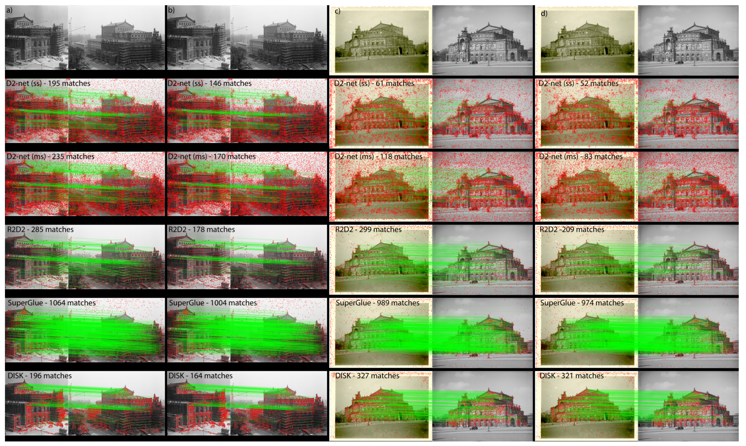
4.2.1. Feature Detection and Matching

Distinctive feature detection and matching in historical image pairs with large radiometric and geometric differences is a difficult task. Specialized feature detectors have to be used to enable successful feature matching [17]. This contribution compares five different feature matching methods on eight different datasets. The aim is, firstly, to maximize the quality of the feature detection and matching, and secondly, to make the different methods comparable.

From a user’s perspective, we try to follow the descriptions and recommendations given in the corresponding publications and do not change elementary parts like the proposed matching method. In the following, a brief explanation of each method is given (see also Section 2) in the order of their publication and all modifications and parameter changes are explained. An example for detected keypoints by the different methods is given exemplarily for two historical images in the appendix (Figure A1). The process of feature detection and matching for the large datasets with approximately 200 images has a runtime of 5 min on a NVIDIA V100 GPU (DISK implementation). In contrast, the slowest approach is the D2-net multiscale implementation which runs only on one CPU and takes around 60 min for the same amount of images. All implementations are based on sequential processing of the images. Thus, there is plenty room for optimization (parallelization, GPU usage), which was not part of this investigation.

D2-Net (Single-Scale and Multiscale)

D2-Net jointly detects and describes features using a CNN [38]. In our experiments, we use the precomputed fine-tuned Caffe VGG16 [42] weights trained on the MegaDepth dataset [54] by [38] (d2_tf.pth). Features are calculated for every single image using the single-scale and the multiscale approach of D2-Net, respectively. The single-scale (-ss) option only processes the input image with a default maximum image width of 1600 pixels. The multiscale (-ms) approach calculates multiple sets of feature maps for an image pyramid consisting of half resolution, full resolution, and double resolution of the input image. The derived feature maps are resized according to the selected resolution using bilinear interpolation, enabling keypoint detection across the different resolutions.

For matching the detected features the proposed approach by [38] is used. Outliers are removed using a mutual nearest neighbor matching including Lowe’s ratio test [23]. That means, features are only kept as matches if the feature point $P_m$ in image i maps only to the feature point $P_n$ in image j and vice versa. Additionally, the distance to the second-closest neighbor has to be smaller than a certain ratio threshold [38] recommend a threshold of $0.90$ for the off-the-shelf descriptors and $0.95$ for the fine-tuned ones. The application on historical images has shown that this threshold is critical for retrieving robust results [8]. Considering these findings, the threshold was slightly modified using $0.96$ for the single-scale and $0.97$ for the multiscale approach.

R2D2

R2D2 also jointly detects and describes features but uses two different layer structures to obtain a different map for reliability and repeatability of the features [39]. In our experiments, we use the precomputed model from [39]. The model was trained with Web images (W), Aachen day-time images (A), Aachen day-night synthetic pairs (S), and Aachen optical flow pairs (F) and can be obtained via https://github.com/naver/r2d2, accessed on 20 September 2021 under the name r2d2_WASF_N16.pt. Features are then extracted using slight modifications. The maximum image width is set to 1600 pixels and the maximum number of keypoints is fixed to 4096 to allow a better comparison to the other approaches.

For matching the obtained keypoints a simple mutual nearest neighbor approach without a threshold is used, similarly done in the experiments by [39].

SuperGlue

SuperGlue [40] combines a feature matching method using a graph neural network with the feature detector SuperPoint [32] in an end-to-end pipeline. In our experiments, we use the precomputed outdoor weights (superglue_outdoor.pth) trained on the MegaDepth dataset. Furthermore, we use the pipeline in https://github.com/cvg/Hierarchical-Localization, accessed on 20 September 2021 and allow a maximum image size of 1600 instead of 1024 for the superpoint_aachen configuration (cf. [55]). The maximum number of detected keypoints is kept at the default value of 4096 for a fair comparison.

DISK

DISK is an end-to-end pipeline to learn local features relying on the policy gradient approach [41]. The network is trained on the MegaDepth dataset [54] and we use the provided weights for our experiments. As the pipeline requires an input size of a multiple of 16 we use an image size of 1600 × 1600 pixels. Additionally, the maximum number of detected keypoints is set to 4096. The recommended ratio threshold of 0.95 is used for matching the features.

4.2.2. Geometric Verification and Camera Pose Estimation

Almost all feature matching methods described, recommend the use of COLMAP for geometric verification of the features and calculation of the camera pose using the integrated bundle adjustment. As already shown, COLMAP is also used to reconstruct the camera positions from the benchmark datasets in a similar workflow (see Section 4.1.1).

Geometric verification implies, that for every image pair combination with feature matches derived by the prior methods, a Fundamental Matrix is calculated. If a minimum of 15 inliers is found via locally optimized RANSAC (LORANSAC) [56] the image pair is considered valid and added to the scene graph (cf. [50]). The scene graph holds the geometrically verified image pairs, their associated inlier correspondences and their geometric relation (cf. [50]).

This structure is used to determine an initial image pair and incrementally register new images. The triangulated points and the derived camera poses are improved in a bundle adjustment with a maximum number of 100 iterations.

To improve the absolute number of registered images, two-view tracks are allowed in our workflow. That means, that features are used for the reconstruction even if they are only detected in two images (i.e., one image pair). For all historical images some assumptions have to be made. A simple radial camera model is chosen, modeling the principal distance (focal length) f, principal point coordinates $c_x$, $c_y$ and only one radial distortion parameter k. As an initial approximation, f is set per default to $f=1.25·max(widt{h}_{px},heigh{t}_{px})$ and $c_x$, $c_y$ lie in the image center.

These assumptions could be far off estimates considering that historical images have to be digitized and the geometric relation to the principal point’s coordinates as well as to the principal distance is completely lost in the process. This may produce outliers which could not be filtered by the benchmark datasets because the same approximations are made for that approach.

As a result, the workflow provides one (or sometimes multiple) model(s) for each of the eight datasets. The model consists of the oriented images and their translation and rotation in the local coordinate system. Each image is introduced as a separate camera and the adjusted interior orientation can be exported. Additionally, a sparse point cloud is created and the number of 3D points, the reprojection error and further statistics are shown in COLMAP.

4.3. Results and Evaluation

All feature matching methods used, are evaluated by the number of oriented images, the pose error (i.e., euclidean distance between benchmark and estimated projection centers) and the angle error $\alpha$ in degree as in Equation (2),

$$2·cos\left(\alpha \right)=\mathrm{trace}\left(R_{\mathrm{benchmark}}^{-1}{R}_{\mathrm{est}}\right)-1,$$

(2)

where $R_{\mathrm{benchmark}}$ and $R_{\mathrm{est}}$ denote the Rotation matrices of the benchmark solution and the estimated solution, respectively. As in refs. [27,57,58] the angle error is our main error metric to evaluate the results of the different reconstructions. Therefore, the reconstruction solution derived by the different methods has to be aligned with the benchmark poses. This requires a seven-parameter transformation (Helmert transformation) from the local coordinate frame of the automatic estimated solution into the local coordinate frame of the benchmark solution. This contribution uses the functionality of COLMAP to compute the alignment between the two reconstructions.

Images that are registered in both reconstructions are selected and an alignment is estimated using LORANSAC and the corresponding projection center coordinates. After that, the alignment is verified by reprojecting common 3D point observations. For LORANSAC a threshold has to be set to distinguish between inlier and outlier camera positions. This threshold is intentionally set to 0.05, which is slightly higher than necessary, to enable the transformation to the benchmark for almost all datasets. Then, it is possible to determine the quality and accuracy of the respective reconstruction using the mean and median values of the pose and angle errors. Lowering the LORANSAC threshold often leads to the result, that the two reconstructions cannot be aligned because there are too many outliers and no further statements about the accuracy could be made.

After the alignment, the mean pose and angle error are calculated for every corresponding image of both reconstructions. Additionally, the median is calculated over all angle errors. Here, the median provides a measure, whether the whole scene reconstruction is not well aligned or whether there are only few or even no incorrect camera positions. Since the pose error is dependent on the scale of the reconstruction it can be compared for all methods within a single dataset only. All results are shown in

Table 3. Results of different feature matching procedures tested on eight datasets in comparison to benchmark data. Table shows respectively number of oriented images, reprojection error in pixels, Euclidean distance (scale-less) and angle error in degree. Best results are highlighted in bold.

	Dataset and Parameters	D2-Net-ss	D2-Net-ms	R2D2	SuperGlue	DISK
Crowngate (20 images)	Oriented images	17	18	12	19	18
	Reproj. error	1.1	1.2	0.9	1.3	0.9
	Pose error (mean)	8245.1	5.5	0.9	0.8	11.7
	Angle error (mean)	173.3	169.9	12.5	4.3	172.8
	Angle error (median)	174.1	173.3	10.7	4.0	172.6
Hofkirche (33 images)	Oriented images	27	28	NA	30	25
	Reproj. error	1.0	1.0	NA	1.3	0.8
	Pose error (mean)	4.8	4.6	NA	5.0	5.1
	Angle error (mean)	93.1	106.5	NA	88.5	92.2
	Angle error (median)	80.7	102.6	NA	108.6	153.3
Moritzburg (23 images)	Oriented images	20	13	14	23	20
	Reproj. error	1.1	1.1	0.8	1.2	0.8
	Pose error (mean)	3.4	6.2	2.9	1.7	0.7
	Angle error (mean)	33.0	159.3	43.7	5.8	7.2
	Angle error (median)	30.1	159.6	42.9	0.8	2.6
Semperoper (20 images)	Oriented images	19	19	14	20	19
	Reproj. error	1.0	1.1	0.8	1.2	0.8
	Pose error (mean)	16,042.5	0.9	2.2	0.3	0.3
	Angle error (mean)	7.8	7.3	7.1	3.0	2.1
	Angle error (median)	3.1	3.2	7.6	3.0	2.1
Crowngate (188 images, 12 in common)	Oriented images	175	178	178	184	183
	Reproj. error	1.3	1.4	1.1	1.4	1.1
	Pose error (mean)	3.6	1.1	1.2	1.2	0.8
	Angle error (mean)	164.0	65.6	176.9	169.4	10.2
	Angle error (median)	164.8	65.6	177.4	169.1	10.7
Hofkirche (176 images, 15 in common)	Oriented images	155	160	166	157	150
	Reproj. error	1.3	1.3	1.0	1.4	1.1
	Pose error (mean)	2.9	2.6	2.6	2.1	3.8
	Angle error (mean)	76.1	74.5	73.4	70.7	71.3
	Angle error (median)	7.4	6.0	4.0	5.7	2.6
Moritzburg (200 images, 15 in common)	Oriented images	129	151	NA	176	155
	Reproj. error	1.4	1.4	NA	1.3	1.0
	Pose error (mean)	0.7	2.2	NA	0.5	0.3
	Angle error (mean)	5.2	66.3	NA	4.2	2.0
	Angle error (median)	4.7	66.2	NA	4.1	1.8
Semperoper (197 images, 10 in common)	Oriented images	135	135	150	167	148
	Reproj. error	1.2	1.2	0.9	1.3	0.9
	Euclidean distance	1.9	0.8	0.4	0.3	0.3
	Angle error (mean)	111.2	6.1	2.5	2.6	2.8
	Angle error (median)	110.8	6.1	2.3	2.5	2.6

.

The analysis of the different models and their resulting error values allows to draw the following conclusions. First of all, it seems that the reprojection error is not a significant value to estimate the correct position and rotation of the historical images. For all different COLMAP models it varies between 0.8 and 1.4 but has no or only a small impact on the result, which is better described by the distance and error measures.

Especially, a combination of both error measures—in this particular case a mean pose error $<1.0$ and a mean angle error $<5.0$°—provides also visually good reconstruction results with no outlier camera positions and orientations. These values are in a range comparable to other state-of-the-art unordered datasets [27,57,58]. Table 3 also shows that for all datasets, DISK and/or SuperGlue provide the highest number of oriented images as well as the most accurate results.

R2D2 performs very good on the Semperoper retrieval datasets but otherwise falls behind the two other methods. As already expected, the Crowngate and Hofkirche datasets are the most difficult to process for the methods. As the Crowngate shows a very symmetric structure all methods are mixing left- and right-side as well as exterior and interior views of the building also shown by angle errors close to 180°.

SuperGlue produces the only valid reconstruction for the Crowngate benchmark dataset while DISK is able to process the retrieval dataset still including multiple incorrectly registered images, which is reflected in the angle error of approximately 10°. For the Hofkirche dataset similar deviations from the real scene occur. The methods are not able to close the large viewpoint gap between the front of the building and the western side (see Figure 3).

This results in an erroneous pose estimation of images and the creation of multiple point clouds of the Hofkirche in one single reconstruction. For this particular building, it could be an option to close the gap using contemporary images to improve the image registration [4].

All methods are able to additionally filter the results of the image retrieval, e.g., for the Semperoper, 197 images are found by LEA. About 15 photographs show the old opera house before 1878, plans or drawings which are not included in the models because they are filtered during geometric verification. However, COLMAP is able to assign these 15 image to a separate reconstruction during bundle adjustment. In conclusion, the described method (LEA+SuperGlue/DISK) enables a completely automatic selection and registration of historical images if the landmark is photographed from multiple surrounding viewpoints.

5. Conclusions and Future Work

Basically, image retrieval applied to historical image works can provide assistance to the researcher for automation within a hand-crafted working process. For example, we demonstrated that LEA is able to generate large historical datasets, which would be an extremely time-consuming task using conventional metadata search. Therefore, the approach requires calculation on a GPU to be effectively implemented in practice, which refers especially to the feature extraction based on a CNN for instance retrieval. The usage of transfer learning (i.e., using a pretrained CNN) is very advantageous and drastically reduces the preparation time. All experiments carried out had a runtime of 5–30 min, depending on the concrete parameterization, i.e., retrieving a single query image within approximately 1000 reference images takes 10–30 s.

Regarding the image retrieval, there are the following concluding remarks. LEA is less sophisticated, but produces better results than DELF. More precisely, the DELF approach with its optimized consideration of local features and a geometric verification did not lead to a substantial improvement of retrieval results. In contrast to LEA and [15], the original parameters for DELF from [19] turned out not to be optimal and esp. DELF led to better results with different parameters. Both approaches lie behind the publications by [15,19] in absolute numbers for mAP. The reason for these differences is most likely due to the underlying data: the pretrained networks used (ResNet50 and VGG-16) were trained on data that included historic buildings, but not historic photographs from a technical point of view. This aspect extends the statement from (p. 1240, [14]) by a more technical dimension, who tell that the used datasets for image retrieval usually refer to a particular type of instances such as landmarks or indoor objects, etc. The results are not based on a benchmark dataset, but on real, heterogeneous use-case data. Overall, there is still potential for improvement, but the approaches under consideration are already delivering practically relevant gains and making the impossible possible—fully automatic pose estimation of historical images.

It was shown that the image retrieval pipeline can be directly used to receive a large number of relevant images of one building by just selecting three query images. The tests have demonstrated that about 160 out of 190 relevant images can be localized up to scale using an adapted SfM workflow. In previous research, the method D2-net outperformed conventional feature matching methods. However, with the generation of a benchmark dataset and the comparison of several different error metrics, it could be shown that D2-net falls behind more recent methods. The methods SuperGlue and DISK in combination with COLMAP are not only able to match are large amount of images, but are also useful to reject images showing, e.g., different buildings or drawings not suitable for the reconstruction. Especially, for the retrieval datasets Moritzburg and Semperoper, the low mean angle error and the small reprojection error prove the impressing result considering the historical image material. These results could be obtained, though all neural networks were only trained on contemporary image data.

For the Hofkirche, the reconstruction is erroneous because certain perspective views are missing from the image retrieval (also due to their potential absence in the original database). In such a case, where not enough poses could be estimated correctly, we suggest the following strategy: Since the building is still present today, it could be an improvement to close the gap between the main historical views using contemporary images or even generate a contemporary SfM model for comparison.

The established benchmark dataset is to the knowledge of the authors the first dataset available which uses only historical images. The dataset can be easily extended by selecting more tie points and/or historical images and the obtainable data allows to reproduce the published results and also further metrics like homographies or depth maps of the historical image pairs. As the creation of such benchmark data is very time-consuming, this dataset may be of great benefit for the Cultural Heritage community.

For further development of the workflow the following aspects/ideas can be considered. An extension for optimizing the image retrieval results—when using multiple query images—could be an aggregation of the result lists. Note that different retrieval goals can be pursued by using appropriate query images. Thereby, query images can be quite similar in some sense but it also makes sense to use very distinct images. The whole end-to-end pipeline is currently being implemented in a scientific environment while a commercial use is not intended at the moment. Especially for the final web application, it is planned to directly integrate the obtained camera positions and orientations by applying a Helmert Transformation on the automatically retrieved poses. This is still under testing and would allow texture projection as well as immersive coloring of 3D models using historical images.

References

1. Niebling, F.; Bruschke, J.; Messemer, H.; Wacker, M.; von Mammen, S. Analyzing Spatial Distribution of Photographs in Cultural Heritage Applications. In Visual Computing for Cultural Heritage; Springer International Publishing: Cham, Switzerland, 2020; pp. 391–408. [Google Scholar] [CrossRef]
2. Evens, T.; Hauttekeete, L. Challenges of digital preservation for cultural heritage institutions. J. Librariansh. Inf. Sci. 2011, 43, 157–165. [Google Scholar] [CrossRef]
3. Münster, S.; Kamposiori, C.; Friedrichs, K.; Kröber, C. Image libraries and their scholarly use in the field of art and architectural history. Int. J. Digit. Libr. 2018, 19, 367–383. [Google Scholar] [CrossRef]
4. Maiwald, F.; Vietze, T.; Schneider, D.; Henze, F.; Münster, S.; Niebling, F. Photogrammetric analysis of historical image repositories for virtual reconstruction in the field of digital humanities. Int. Arch. Photogramm. Remote Sens. Spat. Inf. Sci. 2017, 42, 447. [Google Scholar] [CrossRef] [Green Version]
5. Bevilacqua, M.G.; Caroti, G.; Piemonte, A.; Ulivieri, D. Reconstruction of lost Architectural Volumes by Integration of Photogrammetry from Archive Imagery with 3-D Models of the Status Quo. Int. Arch. Photogramm. Remote Sens. Spat. Inf. Sci. 2019, XLII-2/W9, 119–125. [Google Scholar] [CrossRef] [Green Version]
6. Condorelli, F.; Rinaudo, F. Cultural Heritage Reconstruction From Historical Photographs And Videos. Int. Arch. Photogramm. Remote Sens. Spat. Inf. Sci. 2018, XLII-2, 259–265. [Google Scholar] [CrossRef] [Green Version]
7. Kalinowski, P.; Both, F.; Luhmann, T.; Warnke, U. Data Fusion of Historical Photographs with Modern 3D Data for an Archaeological Excavation—Concept and First Results. Int. Arch. Photogramm. Remote Sens. Spat. Inf. Sci. 2021, XLIII-B2-2021, 571–576. [Google Scholar] [CrossRef]
8. Maiwald, F.; Maas, H.G. An automatic workflow for orientation of historical images with large radiometric and geometric differences. Photogramm. Rec. 2021, 36, 77–103. [Google Scholar] [CrossRef]
9. Snavely, N.; Seitz, S.M.; Szeliski, R. Photo tourism: Exploring photo collections in 3D. ACM Trans. Graph. 2006, 25, 835–846. [Google Scholar] [CrossRef]
10. Schindler, G.; Dellaert, F. 4D Cities: Analyzing, Visualizing, and Interacting with Historical Urban Photo Collections. J. Multimed. 2012, 7, 124–131. [Google Scholar] [CrossRef] [Green Version]
11. Datta, R.; Joshi, D.; Li, J.; Wang, J.Z. Image Retrieval: Ideas, Influences, and Trends of the New Age. ACM Comput. Surv. 2008, 40, 1–60. [Google Scholar] [CrossRef]
12. Sharif Razavian, A.; Azizpour, H.; Sullivan, J.; Carlsson, S. CNN Features Off-the-Shelf: An Astounding Baseline for Recognition. In Proceedings of the IEEE Conference on Computer Vision and Pattern Recognition (CVPR) Workshops, Columbus, OH, USA, 23–28 June 2014. [Google Scholar]
13. Wan, J.; Wang, D.; Hoi, S.C.H.; Wu, P.; Zhu, J.; Zhang, Y.; Li, J. Deep learning for content-based image retrieval: A comprehensive study. In Proceedings of the 22nd ACM International Conference on Multimedia, Orlando, FL, USA, 3–7 November 2014; pp. 157–166. [Google Scholar] [CrossRef]
14. Zheng, L.; Yang, Y.; Tian, Q. SIFT Meets CNN: A Decade Survey of Instance Retrieval. IEEE Trans. Pattern Anal. Mach. Intell. 2018, 40, 1224–1244. [Google Scholar] [CrossRef] [Green Version]
15. Razavian, A.S.; Sullivan, J.; Carlsson, S.; Maki, A. Visual instance retrieval with deep convolutional networks. ITE Trans. Media Technol. Appl. 2016, 4, 251–258. [Google Scholar] [CrossRef] [Green Version]
16. Zeiler, M.D.; Fergus, R. Visualizing and understanding convolutional networks. In Proceedings of the European Conference on Computer Vision, Zurich, Switzerland, 6–12 September 2014; Springer: Berlin/Heidelberg, Germany, 2014; pp. 818–833. [Google Scholar] [CrossRef] [Green Version]
17. Maiwald, F.; Bruschke, J.; Lehmann, C.; Niebling, F. A 4D information system for the exploration of multitemporal images and maps using photogrammetry, web technologies and VR/AR. Virtual Archaeol. Rev. 2019, 10, 1–13. [Google Scholar] [CrossRef]
18. Münster, S.; Lehmann, C.; Lazariv, T.; Maiwald, F.; Karsten, S. Toward an Automated Pipeline for a Browser-Based, City-Scale Mobile 4D VR Application Based on Historical Images; Springer: Berlin/Heidelberg, Germany, 2021. [Google Scholar] [CrossRef]
19. Noh, H.; Araujo, A.; Sim, J.; Weyand, T.; Han, B. Large-scale image retrieval with attentive deep local features. In Proceedings of the IEEE International Conference on Computer Vision, Venice, Italy, 22–29 October 2017; pp. 3456–3465. [Google Scholar] [CrossRef] [Green Version]
20. Fischler, M.A.; Bolles, R.C. Random sample consensus: A paradigm for model fitting with applications to image analysis and automated cartography. Commun. ACM 1981, 24, 381–395. [Google Scholar] [CrossRef]
21. Winder, S.A.J.; Brown, M. Learning Local Image Descriptors. In Proceedings of the 2007 IEEE Conference on Computer Vision and Pattern Recognition, Minneapolis, MN, USA, 17–22 June 2007; pp. 1–8. [Google Scholar] [CrossRef]
22. Sattler, T.; Weyand, T.; Leibe, B.; Kobbelt, L. Image Retrieval for Image-Based Localization Revisited. In Proceedings of the British Machine Vision Conference, Surrey, UK, 3–7 September 2012; Volume 1, p. 4. [Google Scholar]
23. Lowe, D.G. Distinctive image features from scale-invariant keypoints. Int. J. Comput. Vis. 2004, 60, 91–110. [Google Scholar] [CrossRef]
24. Balntas, V.; Lenc, K.; Vedaldi, A.; Mikolajczyk, K. HPatches: A Benchmark and Evaluation of Handcrafted and Learned Local Descriptors. In Proceedings of the 2017 IEEE Conference on Computer Vision and Pattern Recognition (CVPR), Honolulu, HI, USA, 21–26 July 2017. [Google Scholar] [CrossRef] [Green Version]
25. Schönberger, J.L.; Hardmeier, H.; Sattler, T.; Pollefeys, M. Comparative Evaluation of Hand-Crafted and Learned Local Features. In Proceedings of the 2017 IEEE Conference on Computer Vision and Pattern Recognition (CVPR), Honolulu, HI, USA, 21–26 July 2017. [Google Scholar] [CrossRef]
26. Csurka, G.; Dance, C.R.; Humenberger, M. From handcrafted to deep local features. arXiv 2018, arXiv:1807.10254. [Google Scholar]
27. Jin, Y.; Mishkin, D.; Mishchuk, A.; Matas, J.; Fua, P.; Yi, K.M.; Trulls, E. Image Matching Across Wide Baselines: From Paper to Practice. Int. J. Comput. Vis. 2020, 129, 517–547. [Google Scholar] [CrossRef]
28. Sarlin, P.E.; Unagar, A.; Larsson, M.; Germain, H.; Toft, C.; Larsson, V.; Pollefeys, M.; Lepetit, V.; Hammarstrand, L.; Kahl, F.; et al. Back to the Feature: Learning Robust Camera Localization from Pixels to Pose. In Proceedings of the CVPR, Virtual, 19–25 June 2021. [Google Scholar]
29. Jahrer, M.; Grabner, M.; Bischof, H. Learned local descriptors for recognition and matching. In Proceedings of the Computer Vision Winter Workshop, Moravske Toplice, Slovenia, 4–6 February 2008; Volume 2, pp. 39–46. [Google Scholar]
30. Simo-Serra, E.; Trulls, E.; Ferraz, L.; Kokkinos, I.; Fua, P.; Moreno-Noguer, F. Discriminative Learning of Deep Convolutional Feature Point Descriptors. In Proceedings of the International Conference on Computer Vision (ICCV), Santiago, Chile, 7–13 December 2015. [Google Scholar] [CrossRef] [Green Version]
31. Tian, Y.; Fan, B.; Wu, F. L2-Net: Deep Learning of Discriminative Patch Descriptor in Euclidean Space. In Proceedings of the 2017 IEEE Conference on Computer Vision and Pattern Recognition (CVPR), Honolulu, HI, USA, 21–26 July 2017. [Google Scholar] [CrossRef]
32. DeTone, D.; Malisiewicz, T.; Rabinovich, A. SuperPoint: Self-Supervised Interest Point Detection and Description. In Proceedings of the 2018 IEEE/CVF Conference on Computer Vision and Pattern Recognition Workshops (CVPRW), Salt Lake City, UT, USA, 18–23 June 2018; pp. 337–33712. [Google Scholar] [CrossRef] [Green Version]
33. Han, X.; Leung, T.; Jia, Y.; Sukthankar, R.; Berg, A.C. MatchNet: Unifying feature and metric learning for patch-based matching. In Proceedings of the 2015 IEEE Conference on Computer Vision and Pattern Recognition (CVPR), Boston, MA, USA, 7–12 June 2015. [Google Scholar] [CrossRef] [Green Version]
34. Zagoruyko, S.; Komodakis, N. Deep compare: A study on using convolutional neural networks to compare image patches. Comput. Vis. Image Underst. 2017, 164, 38–55. [Google Scholar] [CrossRef]
35. Yi, K.M.; Trulls, E.; Lepetit, V.; Fua, P. LIFT: Learned Invariant Feature Transform. In Proceedings of the Computer Vision—ECCV, Amsterdam, The Netherlands, 11–14 October 2016; pp. 467–483. [Google Scholar] [CrossRef] [Green Version]
36. Mishchuk, A.; Mishkin, D.; Radenović, F.; Matas, J. Working hard to know your neighbor’s margins: Local descriptor learning loss. In Proceedings of the NIPS, Long Beach, CA, USA, 4–9 December 2017. [Google Scholar]
37. Ono, Y.; Trulls, E.; Fua, P.; Yi, K.M. LF-Net: Learning Local Features from Images. In Proceedings of the 32nd International Conference on Neural Information Processing Systems, Montreal, QC, Canada, 3–8 December 2018; Curran Associates Inc.: Red Hook, NY, USA, 2018; pp. 6237–6247. [Google Scholar]
38. Dusmanu, M.; Rocco, I.; Pajdla, T.; Pollefeys, M.; Sivic, J.; Torii, A.; Sattler, T. D2-Net: A Trainable CNN for Joint Detection and Description of Local Features. arXiv 2019, arXiv:1905.03561. [Google Scholar]
39. Revaud, J.; Weinzaepfel, P.; Souza, C.D.; Pion, N.; Csurka, G.; Cabon, Y.; Humenberger, M. R2D2: Repeatable and Reliable Detector and Descriptor. arXiv 2019, arXiv:1906.06195v2. [Google Scholar]
40. Sarlin, P.E.; DeTone, D.; Malisiewicz, T.; Rabinovich, A. SuperGlue: Learning Feature Matching with Graph Neural Networks. In Proceedings of the IEEE/CVF Conference on Computer Vision and Pattern Recognition, Seattle, WA, USA, 16–18 June 2020; pp. 4938–4947. [Google Scholar]
41. Tyszkiewicz, M.J.; Fua, P.; Trulls, E. DISK: Learning local features with policy gradient. arXiv 2020, arXiv:2006.13566. [Google Scholar]
42. Simonyan, K.; Zisserman, A. Very deep convolutional networks for large-scale image recognition. arXiv 2014, arXiv:1409.1556. [Google Scholar]
43. Ronneberger, O.; Fischer, P.; Brox, T. U-Net: Convolutional Networks for Biomedical Image Segmentation. arXiv 2015, arXiv:1505.04597. [Google Scholar]
44. Chollet, F. Deep Learning with Python; Manning Publications: Shelter Island, NY, USA, 2018. [Google Scholar]
45. Jégou, H.; Chum, O. Negative evidences and co-occurences in image retrieval: The benefit of PCA and whitening. In Proceedings of the European Conference on Computer Vision, Florence, Italy, 7–13 October 2012; pp. 774–787. [Google Scholar] [CrossRef]
46. He, K.; Zhang, X.; Ren, S.; Sun, J. Deep residual learning for image recognition. In Proceedings of the IEEE Conference on Computer Vision and Pattern Recognition, Las Vegas, NV, USA, 27–30 June 2016; pp. 770–778. [Google Scholar]
47. Russakovsky, O.; Deng, J.; Su, H.; Krause, J.; Satheesh, S.; Ma, S.; Huang, Z.; Karpathy, A.; Khosla, A.; Bernstein, M.; et al. ImageNet Large Scale Visual Recognition Challenge. Int. J. Comput. Vis. 2015, 115, 211–252. [Google Scholar] [CrossRef] [Green Version]
48. Weyand, T.; Araujo, A.; Cao, B.; Sim, J. Google landmarks dataset v2-a large-scale benchmark for instance-level recognition and retrieval. In Proceedings of the IEEE/CVF Conference on Computer Vision and Pattern Recognition, Seattle, WA, USA, 16–18 June 2020; pp. 2575–2584. [Google Scholar]
49. Ting, K.M. Precision and Recall. In Encyclopedia of Machine Learning and Data Mining; Sammut, C., Webb, G.I., Eds.; Springer US: Boston, MA, USA, 2016; p. 781. [Google Scholar] [CrossRef]
50. Schönberger, J.L.; Frahm, J.M. Structure-from-Motion Revisited. In Proceedings of the 2016 IEEE Conference on Computer Vision and Pattern Recognition (CVPR), Las Vegas, NV, USA, 27–30 June 2016; pp. 4104–4113. [Google Scholar] [CrossRef]
51. Marx, H. Matthäus Daniel Pöppelmann: Der Architekt des Dresdner Zwingers; VEB E.A. Seemann: Leipzig, Germany, 1989. [Google Scholar]
52. Remondino, F.; Nocerino, E.; Toschi, I.; Menna, F. A Critical Review of Automated Photogrammetric Processing of Large Datasets. ISPRS Int. Arch. Photogramm. Remote Sens. Spat. Inf. Sci. 2017, XLII-2/W5, 591–599. [Google Scholar] [CrossRef] [Green Version]
53. OpenStreetMap Contributors. Planet Dump Retrieved from https://planet.osm.org. 2017. Available online: https://www.openstreetmap.org (accessed on 20 September 2021).
54. Li, Z.; Snavely, N. MegaDepth: Learning Single-View Depth Prediction from Internet Photos. In Proceedings of the 2018 IEEE/CVF Conference on Computer Vision and Pattern Recognition, Salt Lake City, UT, USA, 18–23 June 2018; pp. 2041–2050. [Google Scholar] [CrossRef] [Green Version]
55. Sarlin, P.E.; Cadena, C.; Siegwart, R.; Dymczyk, M. From Coarse to Fine: Robust Hierarchical Localization at Large Scale. In Proceedings of the CVPR, Long Beach, CA, USA, 16–20 June 2019. [Google Scholar]
56. Chum, O.; Matas, J.; Kittler, J. Locally Optimized RANSAC. In Pattern Recognition; Michaelis, B., Krell, G., Eds.; Springer: Berlin/Heidelberg, Germany, 2003; pp. 236–243. [Google Scholar] [CrossRef]
57. Sattler, T.; Maddern, W.; Toft, C.; Torii, A.; Hammarstrand, L.; Stenborg, E.; Safari, D.; Okutomi, M.; Pollefeys, M.; Sivic, J.; et al. Benchmarking 6DOF Outdoor Visual Localization in Changing Conditions. In Proceedings of the 2018 IEEE/CVF Conference on Computer Vision and Pattern Recognition, Salt Lake City, UT, USA, 18–22 June 2018. [Google Scholar] [CrossRef] [Green Version]
58. Li, X.; Ling, H. On the Robustness of Multi-View Rotation Averaging. arXiv 2021, arXiv:2102.05454. [Google Scholar]
Figure 1. Example for projection of historical images on simple 3D models (under development) in application VR City https://4dcity.org/, accessed on 20 September 2021.
Ijgi 10 00748 g001
Figure 2. Workflow from an image database to scene reconstruction using image retrieval and photogrammetric methods.
Ijgi 10 00748 g002
Figure 3. All query images used for automatic selection of retrieval datasets using LEA approach.
Ijgi 10 00748 g003
Figure 4. Average precision for MD search and DELF IR over all seven OoI.
Ijgi 10 00748 g004
Figure 5. Selection of PR curves over all OoI for MD search and IR (LEA and DELF). Values in each subfigure refer to AP for MD search and mAP for LEA and DELF aggregating the corresponding PR curves.
Ijgi 10 00748 g005
Figure 6. Average precision for MD search and LEA IR over all seven OoI.
Ijgi 10 00748 g006
Figure 7. Reconstructed camera positions and orientations (small red frustums) derived by COLMAP manually blended into 3D/4D environment of 4D-browser (https://4dbrowser.urbanhistory4d.org/, accessed on 20 September 2021 for better scene understanding. Since there is no 3D model of Schloss Moritzburg yet, the OpenStreetMap [53] representation is used.
Ijgi 10 00748 g007