
Trip Purpose Imputation Using GPS Trajectories with Machine Learning


Institute for Transport Planning and Systems, ETH Zurich, 8093 Zurich, Switzerland
*
Author to whom correspondence should be addressed.
ISPRS Int. J. Geo-Inf. 2021, 10(11), 775; https://0-doi-org.brum.beds.ac.uk/10.3390/ijgi10110775
Submission received: 12 August 2021
/
Revised: 27 October 2021
/
Accepted: 6 November 2021
/
Published: 13 November 2021
Abstract
:We studied trip purpose imputation using data mining and machine learning techniques based on a dataset of GPS-based trajectories gathered in Switzerland. With a large number of labeled activities in eight categories, we explored location information using hierarchical clustering and achieved a classification accuracy of 86.7% using a random forest approach as a baseline. The contribution of this study is summarized below. Firstly, using information from GPS trajectories exclusively without personal information shows a negligible decrease in accuracy (0.9%), which indicates the good performance of our data mining steps and the wide applicability of our imputation scheme in case of limited information availability. Secondly, the dependence of model performance on the geographical location, the number of participants, and the duration of the survey is investigated to provide a reference when comparing classification accuracy. Furthermore, we show the ensemble filter to be an excellent tool in this research field not only because of the increased accuracy (93.6%), especially for minority classes, but also the reduced uncertainties in blindly trusting the labeling of activities by participants, which is vulnerable to class noise due to the large survey response burden. Finally, the trip purpose derivation accuracy across participants reaches 74.8%, which is significant and suggests the possibility of effectively applying a model trained on GPS trajectories of a small subset of citizens to a larger GPS trajectory sample.
1. Introduction
Trip purpose imputation is an important part of constructing travel diaries of individuals and has attracted the attention of many researchers due to its significance in understanding travel behavior, travel demand prediction, and transport planning. The prevalence of GPS-integrated devices provides a large amount of GPS trajectories consisting of a series of longitude-latitude pairs with abundant explicit information (such as travel timing, duration, and location). Nevertheless, the implicit information, such as travel modes and purposes, needs to be imputed to enrich such data for better usage in transport management. While it triggered plenty of studies over past decades [1], most of them focused on mode detection. Although trip purposes can be reported by participants along GPS trajectories, this needs too much effort over a long study duration. In addition, such surveys might suffer from inaccuracy problems due to memory recall issues or the inattention of travelers, and their applicability is still limited to the collected travel diaries. As existing trip purpose imputation studies are mainly confined to small-scale case studies, how to generalize the results into a larger scale continues to be an important research topic and becomes the focus of our work. For comprehensive reviews of research status on trip purpose imputation, readers can consult the studies of Nguyen et al. [2], Ermagun et al. [3], and Gong et al. [4].
The classification performance of different studies depends on many factors, such as sample sizes, survey duration and methods, data sources, activity categories, and data preparation and cleaning steps. For this reason, it is difficult to set a benchmark for comparison across different papers, so we only emphasize innovative aspects of the most recent articles instead of comparing their accuracy rate. In our preliminary research, we found a striking similarity between trip mode and purpose derivation, which are mostly considered separately in the existing literature. While we saw a comparable model performance on these two tasks with similar techniques, this article engages in trip purpose imputation for simplicity and also mentions some relevant progress in mode derivation papers.
While point of interest (POI) information is considered useful in identifying possible activities in a venue, it is not easy to efficiently incorporate such data into an imputation scheme. As a solution, Meng et al. [5] employed social media data (Twitter) to determine the popularities of POI in trip end areas for purpose inference with dynamic Bayesian network models. Scholars in this field seldom investigate the transferability of trained models to other distinguishable datasets, while Gong et al. [6] did look into this aspect. They adopted the Aslan and Zech test and random forests to explore the effects of datasets from different seasons on model performance, and stressed the limited transferability of models across datasets. To maximize the benefits of activity type detection, Ermagun et al. [3] took up the challenge of real-time purpose derivation and advocated the use of Google Places information. To impute trip modes, Yazdizadeh et al. [7] found that a combination of ensemble convolutional neural networks (CNN) and a random forest as a meta learner outperforms single learners like a decision tree, a random forest, or single CNN models.
Although extensive studies have been devoted to the study of trip purpose imputation and there are several comprehensive reviews of this research field, most of them are limited to small-scale case studies and do not consider the generalizability of their imputation scheme. Consequently, the large-scale spatial–temporal characteristics of trip purpose derivation and the problem of mislabeling by participants have not been investigated. Albeit an inverse relationship between sample size and model performance is expected due to the heterogeneity in diverse samples [2], there is a lack of quantitative measures for such phenomenon, which can be used as a guide for comparison across studies and future research design. Moreover, while geographic variables, such as land use information or POIs, can be of benefit, they show large differences among different regions and thus the models using such information are less transferable. Similarly, the benefits of participant-related features come with a survey burden and limited transferability.
Accordingly, our study does not aim at achieving a superior performance to existing methods or improving classification accuracy, but intends to address the practical problems mentioned above. To this end, we propose four research questions: (1) What is the minimum set of data sources for a satisfactory model performance, so that the applicability of the methods can be maximized even with limited data availability? (2) How does the model performance depend on the geographical location, the number of participants, and the duration of the survey? (3) How can we account for the mislabeled activities by participants during the survey? (4) Can a model trained on a relatively small set of data be applied to other data collected from a much larger number of individuals? To the best of our knowledge, this is the first time that such problems are addressed in the trip purpose detection context.
2. Literature Review
2.1. Data Sources
Besides information about location and time collected with GPS-integrated devices, additional data sources are normally included in models to improve travel purpose imputation precision. Generally, the sociodemographic characteristics of participants are gathered together with GPS trajectories and are taken to be important supplementary information [1]. Land use data and POI could be used to indicate possible activities for a stopping point on GPS trajectories [8]. In addition, the popularity of POI inferred from social media data (e.g., Twitter) [5], travel and tourism statistics [9], and mobile phone billing data [10] have also been utilized to derive travel purpose.
2.2. Data Preparation
Data pre-processing, which has been intensively investigated in the data mining field [11], receives much less discussion than it deserves in trip purpose imputation research. Therefore, we discuss the issue in-depth below. García et al. [12] summarized the three most influential data pre-processing requirements to improve data mining efficiency and performance, i.e., imperfect data handling, data reduction, and imbalanced data pre-processing.
An important aspect of imperfect data handling is noise filtering [13], which aims at detecting the attribute noise and the more harmful class noise [14]. For class noise removal, ensemble filters proposed by Brodley and Friedl [15,16] have been widely applied as an excellent tool. Ensemble filters adopt an ensemble of classifiers to eliminate the mislabeled training data that cannot be correctly classified by all or part of the classifiers using n-fold cross-validation. To avoid treating an exception that is specific to an algorithm as noise, multiple algorithms are used. Basically, there are two strategies for implementing ensemble filters: majority vote filters, which mean the instances that cannot be correctly classified by more than half of the algorithms are treated as mislabeled; and conservative consensus filters, which mean only the instances that cannot be correctly classified by all algorithms are treated as noise. Majority vote filters are sometimes preferred to conservative consensus filters, as retaining bad data is more harmful than discarding good data, especially when there are ample training data [16]. Nevertheless, we chose conservative consensus filters, with the results of these two strategies being similar.
Missing data are another typical problem in transport research that normally involves survey processes. The first step to handle missing data should be understanding sources of “unknownness” [17], which might be due to lost, uncollected, or unidentifiable in existing categories. Besides omitting the instances or features with missing values, which is usually not suggested, approaches for missing data inferences can be classified into two groups [18]: data-driven, e.g., mean or mode; and model-based, e.g., k-nearest neighbors (kNN). kNN has gained popularity because of its simplicity and good performance in dealing with both numerical and nominal values [19].
Attribute selection, as a classic part of data reduction, is conducive to generating a simpler and more accurate model and avoiding over-fitting risks [12,20]. For feature selection, feature importance measured by mean decrease in the Gini coefficient in the random forest approach can be used as a reference [21]. However, such a rank-based measure cannot take feature interactions into account and might suffer from stochastic effects [22]. Conventionally, feature selection techniques can be grouped into two categories: filter methods, i.e., variable ranking techniques; and wrapper methods, which involve classifiers and become an NP-hard problem [20]. One of the most popular algorithms for feature selection is minimum redundancy maximum relevance based on mutual information [23], which is initially designed as a filter and then developed to be a wrapper as well [12]. Another popular wrapper algorithm that is designed for the random forest is provided in an R package Boruta [22], which aims at identifying all relevant features rather than an optimal subset and is employed for our analysis.
An imbalanced distribution of categories might result in unbalanced accuracies of classification. This problem also troubled the machine learning community, where Ling and Li [24] suggested duplicating small-portion classes and Kubat and Matwin [25] tried to downsize large-portion classes. One of the most prevalent ways to cope with imbalanced data is the synthetic minority over-sampling technique (SMOTE) introduced by Chawla et al. [26], which suggests formulating new samples as randomized interpolation of minority class samples. SMOTE is widely used because of its simplicity, good performance, and compatibility with any machine learning algorithm [12]. As a variation of SMOTE, adaptive synthetic sampling approach (ADASYN) proposed by He et al. [27] puts more weight on minority samples that are harder to learn when selecting samples for interpolation.
2.3. Classification Techniques
The methods used to derive trip purposes can be divided into two main categories [28]: rule-based systems with an accuracy of around 70% [29], which rely predominantly on land use and personal information, as well as timing, duration, and sequence of activities; and machine learning approaches, which focus more on activities than position and show varying accuracy between 70% and 96% depending on different algorithms, data set, activity categories, and so on [8]. Although manual trip purpose derivation approaches using rules give satisfactory results, there is no standard set of accepted rules for mining travel information and, thus, it relies on researchers’ experiences. Compared to conventional deterministic approaches, machine learning algorithms, such as random forest and dynamic Bayesian network models, could even rank possible activities, which are particularly helpful when activities are ambiguous [5]. Consequently, we opt for machine learning approaches that have already been widely applied in this area, such as decision trees [30], random forests [28], artificial neural networks [31], and dynamic Bayesian network models [5]. Because of the good performance of random forests compared to other methods demonstrated by numerous studies [32,33,34], we employed it as a starting point for analysis. An introduction to random forests is given in Section 3.2.
2.4. Model Performance Assessment
Model performance can be assessed in various ways, which act as an important component of model development. Although reported trip information might suffer from memory recall errors or other issues, it is probably the best candidate as ground-truth for model validation and assessment [35]. Innovatively, Li et al. [36] used the visualized spatial distribution of recognized trip purposes to validate simulation outputs. Albeit classification models might be used to generate travel diaries for citizens that are not in the training dataset, Montini et al. [32] found that the accuracy of trip purpose detection is participant-dependent. As proportion and categories of trip purposes have a significant influence on the accuracy of classification [9], high-frequency activities should be treated with special care.
3. Materials and Methods
3.1. Materials
In this study, we analyzed GPS trajectories collected from 3689 Swiss participants from September 2019 to September 2020 through the “Catch-my-day” GPS tracking app, developed by Motion Tag. Considering solely the 91% of all activities that are within Switzerland, it amounts to 1.82 million activities above a time threshold of 5 min, of which 43% is labeled by participants and used in our following experiments. Although a threshold of 5 min to extract activities from GPS trajectories might ignore some short activities, we use it as a simplification for the current study. As a GPS-integrated mobile phone has a position error of 1 to 50 m with a mean of 6.5 m as shown by Garnett and Stewart [37], this is taken into account when conducting spatial clustering of activities. More details about the study design and research scope can be found in Molloy et al. [38] and Molloy et al. [39].
Based on the “Mobility and Transport Microcensus 2015” in Switzerland, we grouped activities into eight categories as shown in Table 1 with decreasing frequencies of their occurrence. Following “Home” and “Work”, “Leisure” becomes the most frequent activity and involves sophisticated characteristics that require special attention [40,41]. The extracted features are shown in Table 2 and split into three types: personal-based, activity-based, and cluster-based information. The cluster-based information is obtained from each cluster delineated using the hierarchical clustering, which is described in Section 3.2.
Moreover, POI information from Google Places API as adopted in Ermagun et al. [3] was investigated for a pilot study and not considered further due to the large monetary cost for large datasets, such as the one used here and its comparatively minor benefits. Residential zoning information in Switzerland as land use information is also tested with very little effect on trip purpose derivation accuracy and, hence, excluded from the final models.
3.2. Methods
As a classification method, kNN [42] is also shown to be a good missing value imputation technique [12,19]. Here we give a short introduction to the kNN algorithm. Given a training set , where U are predictors and V are labels, we can estimate the distance between a test object and all training objects to find its k nearest neighbors. Then the label for this test object is determined as median of v of its k nearest neighbors in the case of numerical variables and mode in the case of categorical variables. The Gower distance computation between and u, which is applicable for both categorical and continuous variables, can be referred to in Kowarik and Templ [43]. Two issues might affect the performance of kNN: one is the choice of k, where a small value of k could be noise sensitive and a large value of k might include redundant information; another issue is that an arithmetic average might ignore the distance-dependent characteristics, where closer objects have higher similarities. These two issues can be addressed by weighting the vote of each nearest neighbor for the final result by their distance, i.e., weighted kNN. Missing value imputation for personal-related information in this work is conducted using the R package “VIM” developed by Kowarik and Templ [43], which also provides weighted kNN methods for better performance.
To explore implicit information contained in the data, data mining techniques, such as clustering, can be employed [28]. Using the hierarchical clustering method introduced by Ward Jr [44], we grouped the spatial location of activities for each participant to make use of repetitive patterns of human behaviors. Hierarchical clustering optimizes the route by which groups are obtained [45], so it might not give the best clustering result for a specified number of groups [44]. However, compared to another widely known k-means clustering technique, hierarchical clustering allows us to define the distance used for grouping, rather than defining the number of groups. The basic steps for hierarchical clustering are illustrated below: (1) Treat initial x objects as individual clusters; (2) Group a pair of the most “similar” clusters; (3) Repeat step 2 until a single cluster containing all objects is obtained. To define the “similarity” between two clusters, Reference [45] summarized six strategies, from which we selected the “group-average” strategy as it is more reasonable and conservative than its alternatives. In our case, the similarity between two activities is defined as the Euclidean distance of their geographical location. Next, we use two general activity clusters X and Y to illustrate the estimation of their average distance. Assuming there are m and l activities in clusters X and Y, respectively, while i and j are single elements of the m and l activities, respectively. We use to represent the distance between activities i and j, the distance between clusters X and Y. Then we can calculate as:
Through the process of hierarchical clustering, will increase gradually. Therefore, we can define an appropriate threshold to stop the process and get intermediate clustering results. In our study, a threshold of 30 m is chosen to restrict the size of each cluster considering the GPS accuracy [37] and results in a radius of fewer than 30 m for each cluster.
A random forest is an ensemble of classification and regression trees [46]. Since its introduction, classification and regression tree (CART) has been an important tool and received lots of attention in different research fields [42]. A detailed description of CART can be found in Song and Ying [47]. As a further development of CART, Breiman [21] developed the random forest with detailed proofs and experiments based on prior studies.
The process to develop a forest comprises three stages: (1) Bootstrap N sets of samples from and with the same size as training data; (2) Build a decision tree for each sample, and at each node choose the best feature from randomly selected M features; (3) Obtain classification results as the mode of outputs of all trees. As classification algorithms are unstable, this bagging (bootstrap aggregating) process could improve the accuracy of model results [48]. The ensemble method with sampling techniques has also the advantage of more accurate imputation in case of imbalanced distribution across different activities [5]. The classification power and generalization errors of random forests depend on the accuracy and interdependence of each tree, which can be measured by out-of-bag (OOB) errors [49] with two steps: (1) For each tree, predict the data that are not in the bootstrap samples (also called OOB data, about 37% of the training set); (2) Aggregate predictions and calculate error rates.
The advantages of the random forest are multifaceted. Firstly, the generalization error converges with the increase of the number of trees N, so there is no over-fitting problem based on the strong law of large numbers even when N gets large, which allows us to select a large N as long as it is computationally efficient. OOB estimates not only could reveal generalization errors, variable importance, strength and correlation of trees, but also replace a test set, as it is as accurate as using a test set of the same size as the training set. Moreover, OOB estimates are unbiased in contrast to cross-validation with unknown bias. In addition, it is robust in the case of unbalanced class population, missing data, and noise, which often exists in labels of objects [50]. The significance of forest parameters, e.g., N, M, and the maximum final node size of trees, as well as multiple extensions of random forests, are well summarized by Biau and Scornet [51]. Khoshgoftaar et al. [52], suggested default values of and through extensive experiments, where m is the number of features. While many efforts have been devoted to improving the original random forest approach [51,53], the implementation of random forests in this paper is based on a classic R package “randomForest” developed by Liaw and Wiener [54].
In addition to the above-mentioned algorithms, C5.0 [55]—an extension of a well-known classification algorithm C4.5 [56], naive Bayes classifier [57], and multivariate adaptive regression splines (MARS) [58] are adopted because of their satisfactory performance for the implementation of ensemble filters. In our preliminary analysis, principal component analysis for numerical features transformation, support vector machine [59], which is time-consuming for high-dimensional data, and ADASYN [60] were tested, but excluded from further analysis because of limited contributions and high computational requirements. Furthermore, Janzen et al. [10] proposed a multi-stage random forest method as a modification to account for the independence of certain trip purposes on specific tour attributes, but this complicated method did not improve the model performance in our re-implementation.
4. Results
4.1. Initial Analysis Using Random Forests
The performance of random forests can be measured through OOB error rates without splitting the training and test dataset and implementing cross-validation, so we use only labeled data as training data in this subsection for supervised machine learning. Table 3 presents the confusion matrix of labeled versus predicted trip purposes using random forests. We set and as suggested in Khoshgoftaar et al. [52], which approaches the best possible performance in reasonable computation time.
Several important patterns can be observed in Table 3: firstly, an overall accuracy of 86.7% indicates a satisfactory performance of random forests as already demonstrated by numerous studies. Secondly, the accuracy for each activity category decreases approximately in sync with their occurrence frequency except for “Education”. Two reasons might explain this phenomenon: one is that “home”, “work”, and “education” have more regular spatial and temporal patterns, so it is easier to correctly classify them; Another reason is that the imbalanced distribution of these categories makes random forests prefer labeling ambiguous objects as majority classes, as has been discussed by del Río et al. [61]. Another interesting phenomenon in Table 3 is that all categories except “leisure” are most likely to be mislabeled as “leisure”, which involves more complicated characteristics that often make it hard to be distinguished from other categories. In addition, the difference in precision and accuracy might result from specific characteristics of each category: For “home” and “leisure”, accuracy is slightly higher than precision as it is safer for the model to classify ambiguous objects as these majority classes, while accuracies of “errand”, “other”, and “assistance” are lower for the same reason. To better understand the strengths and possible improvement of random forests, we investigate the importance of feature selection, the number of participants and duration of the survey, and spatial characteristics of the accuracy.
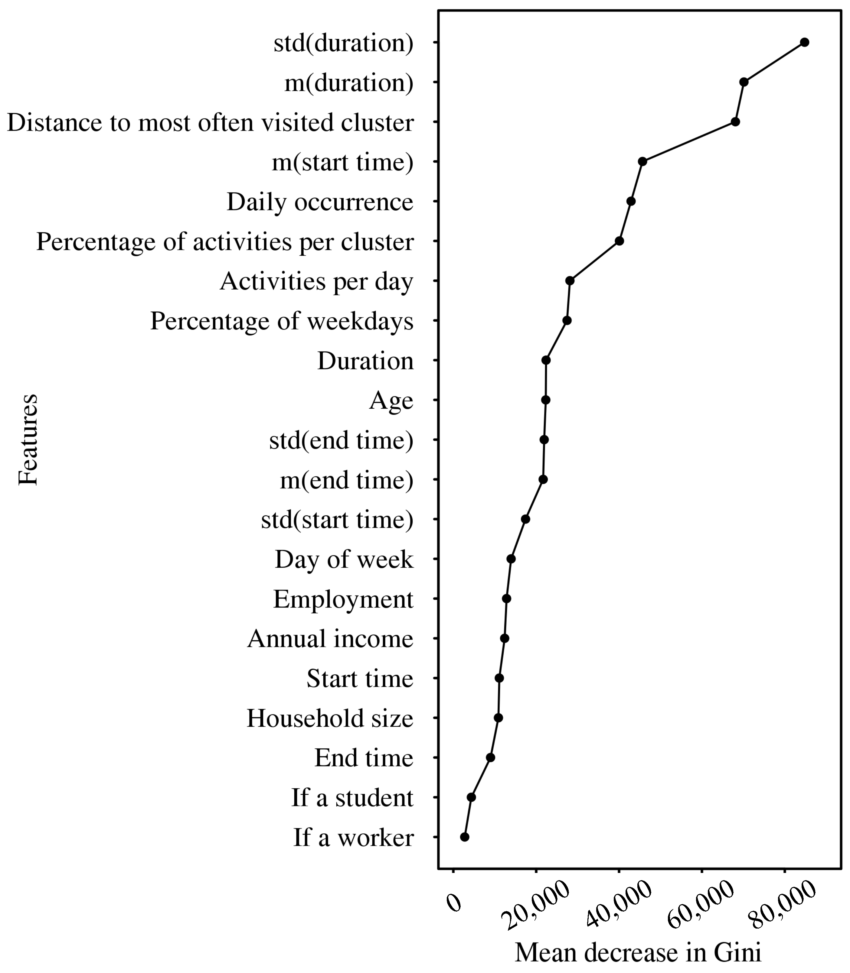
An advantage of the random forest is that it provides an inherent measure of feature importance using Gini impurity as shown in Figure 1, which provides an important reference on feature selection. Among the 21 features, the most important six features are more useful in classification, whereas the personal-based attributes are less relevant: except for “age”, all personal information belongs to the least relevant seven features. To assess the importance of three sets of features grouped in Table 2, we conduct three additional experiments by leaving one set of features out and present the results in Figure 2. When leaving all the personal information unused, the overall accuracy decreased around 0.9%. Although the Boruta method [22] shows that all features are relevant, which indicates a good result of our preliminary feature selection, we omit the personal information from further analysis for the following reasons: This could indicate the strength and applicability of our method even when no personal information is available, i.e., we can undertake trip information enrichment at high accuracy using only GPS trajectories; The inclusion of sociodemographic data might lead to overfitting of models to current participants and limit the applicability of models on GPS trajectories of other users. It is interesting that the elimination of activity information gives similar or even slightly better results compared to using all features, which might result from the intercorrelation or interaction among features. However, the activity information indeed improves the model performance when only cluster-based information is used (not shown), which means the activity information is related to the travel purpose. The removal of cluster-based information leads to a dramatic decrease in model performance, which strongly suggests the effectiveness of our usage of hierarchical clustering algorithms.
Figure 3 shows the spatial distribution of labeled activities and accuracy rate using grids with an area of 4 km in Switzerland. As these two fields have a small correlation coefficient of 0.23, we cannot conclude that higher spatial activity density, which normally means an urban area, will result in a higher accuracy rate. However, the five big cities in Switzerland with higher activity density seem to correspond to a more homogeneous accuracy rate. We can also observe that low activity density areas show large fluctuations in the accuracy rate.
To investigate the dependence of classification performance on the number of participants and the duration of the survey, we extract five groups of participants with different durations of the survey—from 60 to 300 days—during which all activities are labeled as shown in Figure 4. Several interesting patterns can be observed and could provide a reference when comparing results in existing literature with different datasets and designing similar research: longer survey duration leads to higher accuracy, whereas increasing the number of participants deteriorates the accuracy due to more heterogeneous data. When there are only eight participants, the model performance undergoes some fluctuations at a short survey duration. Moreover, there seems to be an upper bound at around 90%. Further research is required to determine whether this upper bound is due to stochastic human behaviors, model ability, incomplete information, or class noise. In the next subsection, we focus on class noise, which has not been discussed in the existing transport literature, due to the smaller datasets available in this research field. It is, however, an essential consideration when dealing with large data sets like ours. We also propose a new criterion in exploring additional features and improving model performance in the next subsection.
4.2. Ensemble Filter with Multiple Classification Algorithms
A large data set is more vulnerable to class noise than smaller ones because of the heavier and longer survey response burden of participants. It is a challenging topic that has not been considered in the context of trip purpose imputation. Although it has been intensively studied in the machine learning field [13,15,62], no perfect solution exists due to a lack of validation information from real data. For our research, we investigate a very popular solution—the ensemble filter—proposed by Brodley and Friedl [15]. The main idea behind the ensemble filter is to identify mislabeled instances that cannot be correctly classified by a set of classifiers. We employ four classifiers with satisfactory performance—random forests, C5.0, Naive Bayes classifiers, and MARS—based on a preliminary test on a pool of algorithms. In this case, we use 10-fold cross-validation to assess model performance. For cross-validation, we also split training and test datasets based on participants, i.e., we test the model performance across participants.
The results are shown in Table 4. For the original labeled data, the random forest gives the best results with an overall accuracy rate of 85.8% and is followed by C5.0 with 84.7%. Naive Bayes classifiers have the lowest accuracy of 57.2%, which is still higher than the suggested threshold (50%) for classifiers in the ensemble filter [16]. Using the strategy of conservative consensus filters in ensemble filters, we removed 8.5% of the labeled data. The model performance improved significantly on these ensemble filtered data −93.6% with random forests and 93.2% with C5.0. These results are promising because of not only the increased accuracy, but also the reduced uncertainties in blindly trusting labels recorded by participants. The minority classes benefit more from this technique as shown in Figure 5, where the accuracy of “Errand”, “Other”, and “Assistance” increased by 23%, 17%, and 29%, respectively. When the model is applied across participants, the accuracy of random forests and C5.0 decreased by about 20% as in Table 4, whereas Naive Bayes classifiers and MARS show nearly no deterioration. The classification accuracy of random forests (74.8%), which is applied across participants on the ensemble filtered data, is an acceptable baseline considering the limited information and inherent difficulties of the across-participants classification. The behavior of Naive Bayes classifiers and MARS in this example might require further exploration in a future study. When one plans to improve the model performance through incorporating more features or investigating new algorithms, considering the model performance across participants should be an essential part to avoid overfitting to a training dataset, which has inherent differences with a test set.
The results in this paper indicate some directions for future research. The trip purpose imputation across participants or across data that are inherently different should still be improved for wider applicability in transport management, where the possibility might exist in including other data sources. While the division of activity categories is primarily subject to practical applications, its effects on model performance could be quantified in further analysis. In addition, the complexity of specific activities like “leisure” can be considered, such as dividing it into several categories.
5. Discussion and Conclusions
To summarize, this paper investigated multiple classification algorithms, including the random forest for trip purpose imputation to enrich GPS trajectories with data mining techniques, such as hierarchical clustering and ensemble filters.
As a baseline, we achieved an overall accuracy rate of 86.7% for eight activity categories using the highly heterogeneous data (3689 participants) with random forests. Through feature importance analysis using the inherent measure of the mean decrease in Gini of random forests and the Boruta method, we verified that current features are of high relevance and the features extracted with hierarchical clustering are crucial in model performance. Additional experiments that leave out a set of personal-related features reveal the possibility of trip purpose imputation with only GPS trajectories. Thanks to the innovative application of hierarchical clustering in extracting relevant features, the answer to the first research question becomes obvious: the required data sources for a satisfactory model performance are minimized to GPS trajectories. Although many researchers managed to achieve better performance by incorporating various data sources, we advocate considering limited data availability on a larger scale, where collecting personal information along with GPS trajectories is impossible or the quality of data sources varies considerably, is vital to generalize our results.
In this context, it is important to note, this is misleading to compare accuracy rates among papers due to the different sample sizes (persons and length of observation periods), activity categories, and data sources. To alleviate this circumstance and provide a reference for the design of similar research, we investigated the dependence of classification performance on the geographical location, the number of participants, and the duration of the survey. Taking advantage of the abundant (780,000) user-labeled activities along GPS trajectories, the spatial distribution of the accuracy rate over Switzerland is visualized. This result is meaningful for densely populated regions where better transport management is required. We show that the model performance in these regions undergoes fewer fluctuations and is more reliable. Furthermore, a longer survey duration helps to improve performance except for the fluctuations when only limited participants are involved over a short period, whereas a larger number of participants results in a higher diversity of the data that are detrimental to model performance, but help improve representativeness.
The employment of the ensemble filter improves model performance significantly from 85.8% to 93.6% with random forests, particularly for minority classes that have lower accuracy due to imbalanced class distribution and complicated characteristics of instances. Besides improving accuracy, the ensemble filter is also effective in reducing errors caused by mislabeling, to which our dataset is vulnerable due to the large response burden imposed on participants.
Another aspect that has not been studied in the existing literature is the trip purpose derivation across participants, where we obtained an accuracy rate of 74.8% using random forests. This result is quite promising, as it indicates that we can apply our trained model using only GPS trajectories and user labels to other GPS trajectories at a much larger scale, without the need to collect additional personal information. As the collection of GPS trajectories exclusively involves much less effort and monetary costs, the applicability of our imputation scheme could be readily expanded, which is significant for transport demand prediction and transport planning at a large scale.
Author Contributions
Conceptualization, Kay W. Axhausen and Joseph Molloy; methodology, Qinggang Gao; software, Qinggang Gao; validation, Qinggang Gao and Joseph Molloy; formal analysis, Qinggang Gao; investigation, Qinggang Gao; resources, Kay W. Axhausen and Joseph Molloy; data curation, Kay W. Axhausen and Joseph Molloy; writing—original draft preparation, Qinggang Gao; writing—review and editing, Kay W. Axhausen and Joseph Molloy; visualization, Qinggang Gao; supervision, Kay W. Axhausen and Joseph Molloy; project administration, Kay W. Axhausen and Joseph Molloy; funding acquisition, Kay W. Axhausen and Joseph Molloy. All authors have read and agreed to the published version of the manuscript.
Funding
The project is funded by the Swiss Innovation Agency (Innosuisse) and the Federal Department of the Environment, Transport, Energy and Communications (DETEC).
Institutional Review Board Statement
Not applicable.
Informed Consent Statement
Not applicable.
Data Availability Statement
The data presented in this study are available on request. The data are not publicly available due to project restrictions.
Conflicts of Interest
The authors declare no conflict of interest. The funders had no role in the design of the study; in the collection, analyses, or interpretation of data; in the writing of the manuscript, or in the decision to publish the results.
References
- Axhausen, K.; Schönfelder, S.; Wolf, J.; Oliveira, M.; Samaga, U. 80 weeks of GPS-traces: Approaches to enriching the trip information. Transp. Res. Rec. 2003, 1870, 46–54. [Google Scholar] [CrossRef]
- Nguyen, M.H.; Armoogum, J.; Madre, J.L.; Garcia, C. Reviewing trip purpose imputation in GPS-based travel surveys. J. Traffic Transp. Eng. 2020, 7, 395–412. [Google Scholar] [CrossRef]
- Ermagun, A.; Fan, Y.; Wolfson, J.; Adomavicius, G.; Das, K. Real-time trip purpose prediction using online location-based search and discovery services. Transp. Res. Part C Emerg. Technol. 2017, 77, 96–112. [Google Scholar] [CrossRef]
- Gong, L.; Morikawa, T.; Yamamoto, T.; Sato, H. Deriving personal trip tata from GPS data: A literature review on the existing methodologies. Procedia Soc. Behav. Sci. 2014, 138, 557–565. [Google Scholar] [CrossRef] [Green Version]
- Meng, C.; Cui, Y.; He, Q.; Su, L.; Gao, J. Towards the Inference of Travel Purpose with Heterogeneous Urban Data. IEEE Trans. Big Data 2019, 1. [Google Scholar] [CrossRef]
- Gong, L.; Kanamori, R.; Yamamoto, T. Data selection in machine learning for identifying trip purposes and travel modes from longitudinal GPS data collection lasting for seasons. Travel Behav. Soc. 2018, 11, 131–140. [Google Scholar] [CrossRef]
- Yazdizadeh, A.; Patterson, Z.; Farooq, B. Ensemble Convolutional Neural Networks for Mode Inference in Smartphone Travel Survey. IEEE Trans. Intell. Transp. Syst. 2020, 21, 2232–2239. [Google Scholar] [CrossRef] [Green Version]
- Deng, Z.; Ji, M. Deriving rules for trip purpose identification from GPS travel survey data and land use data: A machine learning approach. In Proceedings of the 7th International Conference on Traffic and Transportation Studies, Kunming, China, 3–5 August 2010. [Google Scholar] [CrossRef]
- Lu, Y.; Zhang, L. Imputing trip purposes for long-distance travel. Transportation 2015, 42, 581–595. [Google Scholar] [CrossRef]
- Janzen, M.; Vanhoof, M.; Axhausen, K.W. Purpose imputation for long-distance tours without personal information. In Arbeitsberichte Verkehrs-und Raumplanung; ETH Zurich: Zurich, Switzerland, 2016; Volume 1181. [Google Scholar] [CrossRef]
- García, S.; Luengo, J.; Herrera, F. Data Preprocessing in Data Mining; Springer: Berlin, Germany, 2015. [Google Scholar]
- García, S.; Luengo, J.; Herrera, F. Tutorial on practical tips of the most influential data preprocessing algorithms in data mining. Knowl.-Based Syst. 2016, 98, 1–29. [Google Scholar] [CrossRef]
- Frenay, B.; Verleysen, M. Classification in the Presence of Label Noise: A Survey. IEEE Trans. Neural Netw. Learn. Syst. 2014, 25, 845–869. [Google Scholar] [CrossRef]
- Zhu, X.; Wu, X. Class Noise vs. Attribute Noise: A Quantitative Study. Artif. Intell. Rev. 2004, 22, 177–210. [Google Scholar] [CrossRef]
- Brodley, C.E.; Friedl, M.A. Identifying and eliminating mislabeled training instances. In Proceedings of the National Conference on Artificial Intelligence, Portland, OR, USA, 4–8 August 1996; pp. 799–805. [Google Scholar]
- Brodley, C.E.; Friedl, M.A. Identifying mislabeled training data. J. Artif. Intell. Res. 1999, 11, 131–167. [Google Scholar] [CrossRef]
- Kotsiantis, S.B.; Kanellopoulos, D.; Pintelas, P.E. Data preprocessing for supervised leaning. Int. J. Comput. Sci. 2006, 1, 111–117. [Google Scholar]
- Lakshminarayan, K.; Harp, S.A.; Samad, T. Imputation of missing data in industrial databases. Appl. Intell. 1999, 11, 259–275. [Google Scholar] [CrossRef]
- Batista, G.E.; Monard, M.C. An analysis of four missing data treatment methods for supervised learning. Appl. Artif. Intell. 2003, 17, 519–533. [Google Scholar] [CrossRef]
- Chandrashekar, G.; Sahin, F. A survey on feature selection methods. Comput. Electr. Eng. 2014, 40, 16–28. [Google Scholar] [CrossRef]
- Breiman, L. Random forests. Mach. Learn. 2001, 45, 5–32. [Google Scholar] [CrossRef] [Green Version]
- Kursa, M.B.; Rudnicki, W.R. Feature Selection with the Boruta Package. J. Stat. Softw. 2010, 36, 1–13. [Google Scholar] [CrossRef] [Green Version]
- Peng, H.; Long, F.; Ding, C. Feature selection based on mutual information criteria of max-dependency, max-relevance, and min-redundancy. IEEE Trans. Pattern Anal. Mach. Intell. 2005, 27, 1226–1238. [Google Scholar] [CrossRef]
- Ling, C.X.; Li, C. Data mining for direct marketing: Problems and solutions. In Proceedings of the Fourth International Conference on Knowledge Discovery and Data Mining, New York, NY, USA, 27–31 August 1998; Volume 98, pp. 73–79. [Google Scholar]
- Kubat, M.; Matwin, S. Addressing the curse of imbalanced training sets: One-sided selection. In Proceedings of the Fourteenth International Conference on Machine Learning, Nashville, TN, USA, 8–12 July 1997; Volume 97, pp. 179–186. [Google Scholar]
- Chawla, N.V.; Bowyer, K.W.; Hall, L.O.; Kegelmeyer, W.P. SMOTE: Synthetic minority over-sampling technique. J. Artif. Intell. Res. 2002, 16, 321–357. [Google Scholar] [CrossRef]
- He, H.; Bai, Y.; Garcia, E.A.; Li, S. ADASYN: Adaptive synthetic sampling approach for imbalanced learning. In Proceedings of the 2008 IEEE International Joint Conference on Neural Networks (IEEE World Congress on Computational Intelligence), Hongkong, China, 1–6 June 2008. [Google Scholar]
- Montini, L.; Rieser-Schüssler, N.; Horni, A.; Axhausen, K. Trip purpose identification from GPS tracks. Transp. Res. Rec. 2014, 2405, 16–23. [Google Scholar] [CrossRef]
- Shen, L.; Stopher, P.R. A process for trip purpose imputation from Global Positioning System data. Transp. Res. Part C Emerg. Technol. 2013, 36, 261–267. [Google Scholar] [CrossRef]
- Oliveira, M.; Vovsha, P.; Wolf, J.; Mitchell, M. Evaluation of two methods for identifying trip purpose in GPS-based household travel surveys. Transp. Res. Rec. 2014, 2405, 33–41. [Google Scholar] [CrossRef]
- Xiao, G.; Juan, Z.; Zhang, C. Detecting trip purposes from smartphone-based travel surveys with artificial neural networks and particle swarm optimization. Transp. Res. Part C Emerg. Technol. 2016, 71, 447–463. [Google Scholar] [CrossRef]
- Montini, L.; Rieser-Schüssler, N.; Axhausen, K.W. Personalisation in multi-day GPS and accelerometer data processing. In Proceedings of the 14th Swiss Transport Research Conference (STRC 2014), Ascona, Switzerland, 14–16 May 2014. [Google Scholar]
- Gong, L.; Yamamoto, T.; Morikawa, T. Comparison of activity type identification from mobile phone GPS data using various machine learning methods. Asian Transp. Stud. 2016, 4, 114–128. [Google Scholar] [CrossRef]
- Feng, T.; Timmermans, H.J. Detecting activity type from GPS traces using spatial and temporal information. Eur. J. Transp. Infrastruct. Res. 2015, 15, 662–674. [Google Scholar] [CrossRef]
- Liao, L.; Fox, D.; Kautz, H. Extracting places and activities from GPS traces using hierarchical conditional random fields. Int. J. Robot. Res. 2007, 26, 119–134. [Google Scholar] [CrossRef]
- Li, A.; Huang, Y.; Axhausen, K.W. An approach to imputing destination activities for inclusion in measures of bicycle accessibility. J. Transp. Geogr. 2020, 82, 102566. [Google Scholar] [CrossRef]
- Garnett, R.; Stewart, R. Comparison of GPS units and mobile Apple GPS capabilities in an urban landscape. Cartogr. Geogr. Inf. Sci. 2015, 42, 1–8. [Google Scholar] [CrossRef]
- Molloy, J.; Castro Fernández, A.; Götschi, T.; Schoeman, B.; Tchervenkov, C.; Tomic, U.; Hintermann, B.; Axhausen, K.W. A national-scale mobility pricing experiment using GPS tracking and online surveys in Switzerland. Response rates and survey method results. Arbeitsberichte-Verkehrs-Und Raumplanung 2020, 1555. [Google Scholar] [CrossRef]
- Molloy, J.; Tchervenkov, C.; Schatzmann, T.; Schoeman, B.; Hintermann, B.; Axhausen, K.W. MOBIS-COVID19/25. Results as of 19/10/2020 (Post-Lockdown). 2020. Available online: https://0-doi-org.brum.beds.ac.uk/10.3929/ethz-b-000447684 (accessed on 9 November 2021).
- Schlich, R.; Schönfelder, S.; Hanson, S.; Axhausen, K. Structures of Leisure Travel: Temporal and Spatial Variability. Transp. Rev. 2004, 24, 219–237. [Google Scholar] [CrossRef]
- Stauffacher, M.; Schlich, R.; Axhausen, K.W.; Scholz, R.W. The diversity of travel behaviour: Motives and social interactions in leisure time activities. Arbeitsberichte-Verkehrs-Und Raumplanung 2005, 328. [Google Scholar] [CrossRef]
- Wu, X.; Kumar, V. The Top Ten Algorithms in Data Mining; CRC Press: Boca Raton, FL, USA, 2009. [Google Scholar]
- Kowarik, A.; Templ, M. Imputation with the R Package VIM. J. Stat. Softw. 2016, 74, 1–16. [Google Scholar] [CrossRef] [Green Version]
- Ward, J.H., Jr. Hierarchical grouping to optimize an objective function. J. Am. Stat. Assoc. 1963, 58, 236–244. [Google Scholar] [CrossRef]
- Lance, G.N.; Williams, W.T. A general theory of classificatory sorting strategies: 1. hierarchical systems. Comput. J. 1967, 9, 373–380. [Google Scholar] [CrossRef] [Green Version]
- Breiman, L.; Friedman, J.; Stone, C.J.; Olshen, R.A. Classification and Regression Trees; CRC Press: Boca Raton, FL, USA, 1984. [Google Scholar]
- Song, Y.Y.; Ying, L.U. Decision tree methods: Applications for classification and prediction. Shanghai Arch. Psychiatry 2015, 27, 130. [Google Scholar]
- Breiman, L. Bagging predictors. Mach. Learn. 1996, 24, 123–140. [Google Scholar] [CrossRef] [Green Version]
- Breiman, L. Out-of-Bag Estimation; Technical Rerport; Department of Statistics, University of California: Berkeley, CA, USA, 1996. [Google Scholar]
- Breiman, L.; Cutler, A. Manual—Setting Up, Using, and Understanding Random Forests V4.0. 2003. Available online: https://www.stat.berkeley.edu/~breiman/Using_random_forests_v4.0.pdf (accessed on 9 November 2021).
- Biau, G.; Scornet, E. A random forest guided tour. Test 2016, 25, 197–227. [Google Scholar] [CrossRef] [Green Version]
- Khoshgoftaar, T.M.; Golawala, M.; Van Hulse, J. An empirical study of learning from imbalanced data using random forest. In Proceedings of the 19th IEEE International Conference on Tools with Artificial Intelligence (ICTAI 2007), Patras, Greece, 29–31 October 2007; Volume 2, pp. 310–317. [Google Scholar]
- Abellán, J.; Mantas, C.J.; Castellano, J.G.; Moral-García, S. Increasing diversity in random forest learning algorithm via imprecise probabilities. Expert Syst. Appl. 2018, 97, 228–243. [Google Scholar] [CrossRef]
- Liaw, A.; Wiener, M. Classification and regression by randomForest. R News 2002, 2, 18–22. [Google Scholar]
- Pang, S.L.; Gong, J.Z. C5.0 Classification Algorithm and Application on Individual Credit Evaluation of Banks. Syst. Eng. Theory Pract. 2009, 29, 94–104. [Google Scholar] [CrossRef]
- Quinlan, J.R. C4.5: Programs for Machine Learning; Morgan Kaufmann Publishers Inc.: San Francisco, CA, USA, 1993. [Google Scholar]
- Meyer, D.; Dimitriadou, E.; Hornik, K.; Weingessel, A.; Leisch, F.; Chang, C.C.; Lin, C.C.; Meyer, M.D. Package ‘e1071’. 2019. Available online: https://cran.r-project.org/web/packages/e1071/e1071.pdf (accessed on 9 November 2021).
- Friedman, J.H. Multivariate Adaptive Regression Splines. Ann. Stat. 1991, 19, 1–67. [Google Scholar] [CrossRef]
- Karatzoglou, A.; Smola, A.; Hornik, K.; Zeileis, A. kernlab-an S4 package for kernel methods in R. J. Stat. Softw. 2004, 11, 1–20. [Google Scholar] [CrossRef] [Green Version]
- Branco, P.; Ribeiro, R.P.; Torgo, L. UBL: An R package for utility-based learning. arXiv 2016, arXiv:1604.08079. [Google Scholar]
- Del Río, S.; López, V.; Benítez, J.M.; Herrera, F. On the use of MapReduce for imbalanced big data using Random Forest. Inf. Sci. 2014, 285, 112–137. [Google Scholar] [CrossRef]
- Guan, D.; Yuan, W. A Survey of mislabeled training data detection techniques for pattern classification. IETE Tech. Rev. 2013, 30, 524–530. [Google Scholar] [CrossRef]
Figure 1.
Feature importance in trip purpose imputation measured with mean decrease in Gini in random forests.
Figure 1.
Feature importance in trip purpose imputation measured with mean decrease in Gini in random forests.

Figure 2.
The model performance for each activity category and the overall accuracy in four experiments, where we use all features, or leave one set of features unused to measure the significance of each set of features.
Figure 2.
The model performance for each activity category and the overall accuracy in four experiments, where we use all features, or leave one set of features unused to measure the significance of each set of features.

Figure 3.
The spatial distribution of the number of labeled activities (a) and classification accuracy of the random forest (b). Each grid has an area of 4 km in Switzerland. The exponential scale in (a) is used to account for the unevenly distributed activities.
Figure 3.
The spatial distribution of the number of labeled activities (a) and classification accuracy of the random forest (b). Each grid has an area of 4 km in Switzerland. The exponential scale in (a) is used to account for the unevenly distributed activities.

Figure 4.
The impact of the number of participants and the duration of the survey on model performance.
Figure 4.
The impact of the number of participants and the duration of the survey on model performance.

Figure 5.
The model performance on the original data and the ensemble filtered data through four classification algorithms. The accuracy rate is calculated based on the classification results that are voted by the four classification algorithms.
Figure 5.
The model performance on the original data and the ensemble filtered data through four classification algorithms. The accuracy rate is calculated based on the classification results that are voted by the four classification algorithms.


Table 1.
Activity categories.
| Category | Example Activities | Count | Percent |
|---|---|---|---|
| Home | Any activities at home | 293,129 | 16.1 |
| Work | Any activities at work place | 171,329 | 9.4 |
| Leisure | Exercise, travel | 123,735 | 6.8 |
| Shopping | Food, clothing | 64,071 | 3.5 |
| Other | Transfer | 46,413 | 2.5 |
| Errand | Travel for business | 40,119 | 2.2 |
| Assistance | Pick up/drop off | 28,189 | 1.5 |
| Education | University, school | 12,694 | 0.7 |
| Unlabeled | - | 1,041,409 | 57.2 |
| Total | - | 1,821,088 | 100 |
Table 2.
Selected features for trip purpose imputation. The categorical features are indicated by *, while m() and std() denote “mean of” and “standard deviation of”, respectively.
Table 2.
Selected features for trip purpose imputation. The categorical features are indicated by *, while m() and std() denote “mean of” and “standard deviation of”, respectively.
| Personal-Based | Activity-Based | Cluster-Based |
|---|---|---|
| Household size | Duration | m(duration) |
| Employment * | Start time | std(duration) |
| Age | End time | m(start time) |
| Annual income * | Day of week * | std(start time) |
| If a worker * | Activities per day | m(end time) |
| If a student * | - | std(end time) |
| - | - | Percentage of weekdays |
| - | - | Percentage of activities per cluster |
| - | - | Daily occurrence |
| - | - | Distance to most often visited cluster |
Table 3.
Confusion matrix of labeled versus predicted trip purposes using random forests (overall accuracy: 86.7%).
Table 3.
Confusion matrix of labeled versus predicted trip purposes using random forests (overall accuracy: 86.7%).
| Predicted | Home | Work | Leisure | Shopping | Errand | Other | Assistance | Education | Accuracy | Precision | |
|---|---|---|---|---|---|---|---|---|---|---|---|
| Labeled | |||||||||||
| Home | 286,000 | 1980 | 2980 | 937 | 720 | 558 | 384 | 20 | 97.4% | 95.8% | |
| Work | 3670 | 157,000 | 5400 | 1680 | 1490 | 1270 | 362 | 131 | 91.8% | 92.0% | |
| Leisure | 3430 | 3850 | 105,000 | 4670 | 2720 | 2930 | 870 | 190 | 84.9% | 74.0% | |
| Shopping | 1340 | 1960 | 7770 | 47,600 | 2690 | 2130 | 511 | 71 | 74.3% | 74.7% | |
| Errand | 2020 | 2630 | 7700 | 4400 | 27,000 | 1960 | 560 | 107 | 58.3% | 72.7% | |
| Other | 1090 | 1680 | 6870 | 2710 | 1540 | 25,600 | 429 | 192 | 63.9% | 71.7% | |
| Assistance | 913 | 1110 | 5430 | 1590 | 861 | 1030 | 17,200 | 50 | 61.1% | 84.5% | |
| Education | 64 | 448 | 737 | 149 | 145 | 267 | 39 | 10,800 | 85.4% | 93.4% | |
Table 4.
Classification accuracy of multiple algorithms with ensemble filter and across participants imputation.
Table 4.
Classification accuracy of multiple algorithms with ensemble filter and across participants imputation.
| Random Forest | C5.0 | Naive Bayes | MARS | |
|---|---|---|---|---|
| Original data | 85.8% | 84.7% | 57.2% | 66.7% |
| Ensemble filtered (8.5%) data | 93.6% | 93.2% | 61.8% | 73.0% |
| Original data, across participants imputation | 68.0% | 65.4% | 57.2% | 66.6% |
| Ensemble filtered (8.5%) data, across participants imputation | 74.8% | 72.3% | 62.0% | 72.7% |
Publisher’s Note: MDPI stays neutral with regard to jurisdictional claims in published maps and institutional affiliations. |
© 2021 by the authors. Licensee MDPI, Basel, Switzerland. This article is an open access article distributed under the terms and conditions of the Creative Commons Attribution (CC BY) license (https://creativecommons.org/licenses/by/4.0/).
Share and Cite
MDPI and ACS Style
Gao, Q.; Molloy, J.; Axhausen, K.W. Trip Purpose Imputation Using GPS Trajectories with Machine Learning. ISPRS Int. J. Geo-Inf. 2021, 10, 775. https://0-doi-org.brum.beds.ac.uk/10.3390/ijgi10110775
AMA Style
Gao Q, Molloy J, Axhausen KW. Trip Purpose Imputation Using GPS Trajectories with Machine Learning. ISPRS International Journal of Geo-Information. 2021; 10(11):775. https://0-doi-org.brum.beds.ac.uk/10.3390/ijgi10110775
Chicago/Turabian StyleGao, Qinggang, Joseph Molloy, and Kay W. Axhausen. 2021. "Trip Purpose Imputation Using GPS Trajectories with Machine Learning" ISPRS International Journal of Geo-Information 10, no. 11: 775. https://0-doi-org.brum.beds.ac.uk/10.3390/ijgi10110775
Note that from the first issue of 2016, this journal uses article numbers instead of page numbers. See further details here.