Article

Micro-Fabric Analyzer (MFA): A New Semiautomated ArcGIS-Based Edge Detector for Quantitative Microstructural Analysis of Rock Thin-Sections

1
Department of Biological, Geological and Environmental Sciences, University of Catania, 95129 Catania, Italy
2
Institut de Physique du Globe de Paris, Centre National de la Recherche Scientifique (CNRS), Université de Paris, F-75005 Paris, France
*
Author to whom correspondence should be addressed.
ISPRS Int. J. Geo-Inf. 2021, 10(2), 51; https://0-doi-org.brum.beds.ac.uk/10.3390/ijgi10020051
Submission received: 1 December 2020 / Revised: 21 January 2021 / Accepted: 22 January 2021 / Published: 27 January 2021
(This article belongs to the Special Issue Application of Geology and GIS)

Abstract

:
Micro-Fabric Analyzer (MFA) is a new GIS-based tool for the quantitative extrapolation of rock microstructural features that takes advantage both of the characteristics of the X-ray images and the optical image features. Most of the previously developed edge mineral grain detectors are uniquely based on the physical properties of the X-ray-, electron-, or optical-derived images; not permitting the exploitation of the specific physical properties of each image type at the same time. More advanced techniques, such as 3D microtomography, permit the reconstruction of tridimensional models of mineral fabric arrays, even though adjacent mineral grain boundaries with the same atomic density are often not detectable. Only electron backscatter diffraction (EBSD) allows providing high-performing grain boundary detection that is crystallographically differentiated per mineral phase, even though it is relatively expensive and can be executed only in duly equipped microanalytical laboratories by suitably trained users. Instead, the MFA toolbox allows quantifying fabric parameters subdivided per mineral type starting from a crossed-polarizers high-resolution RGB image, which is useful for identifying the edges of the individual grains characterizing rock fabrics. Then, this image is integrated with a set of micro-X-ray maps, which are useful for the quantitative extrapolation of elemental distribution maps. In addition, all this is achieved by means of low-cost and easy-to-use equipment. We applied the tool on amphibolite, mylonitic-paragneiss, and -tonalite samples to extrapolate the particle fabric on different metamorphic rock types, as well as on the same sandstone sample used for another edge detector, which is useful for comparing the obtained results.

1. Introduction

Petrogenetic processes are mostly controlled by chemical–physical counterbalancing factors such as deposition mechanisms vs. diagenesis for sedimentary rocks, emplacement or flow dynamics vs. crystal solidification velocity for plutonic and volcanic rocks, respectively, and deformation vs. recovery processes for metamorphic rocks. In this view, the quantitative restitution of mineralogical composition and fabric arrangement of rock constituents are crucial parameters to be determined in unravelling most of the geological processes.
In the last decade, many efforts have been focused on the development of quantitative extrapolation techniques that are useful for obtaining more increasingly performing rock microstructural features.
All these methods can be summarized in three different groups, which are subdivided in function of the image acquisition physical properties.
The first group is the optical image-derived methods. These methods are based on three crucial points: (a) the image-acquiring methods; (b) the prefiltering process; and (c) the algorithm used for edge detection extraction [1,2,3,4,5,6,7].
The second group is defined as High-resolution X-ray Computed Tomography (HRXCT) or micro-CT (μCT). This is a frequently used non-destructive 3D imaging and analysis technique for the investigation of a large variety of geomaterials, which is based on the differentiated X-ray absorption of a rotating 3D sample [8,9,10,11].
Finally, the third group can be described by the electron backscatter diffraction (EBSD) methods. Electron backscatter diffraction is a method based on the interaction between an electron beam and a crystal lattice where the diffracted electrons create a pattern that can cause specific fluorescent effects. The method provides crystallographic data regarding the microstructure of a sample through the elaboration of the diffraction pattern sensitive to crystal orientation. This method is able to characterize grain boundaries as well as differentiate between crystallographically different phases [12,13,14].
All the optical image-derived methods start from the acquisition of thin section images, which are acquired from an optical microscope or by a high-resolution light polarized scanner. Most of these methods necessitate the stacks of multiple image acquisitions at different crossed polarizers orientation in order to minimize the effect of the boundaries disappearing between two adjacent mineral grains of the same species during rotation [4,6]. The acquiring of the stacked optical image is even more true if it is necessary to acquire images that are useful for computing the preferential orientation of quartz c-axis pattern via the definition of the Achsenverteilungsanalyse (AVA) [15,16,17,18]. In this case, indeed, it is necessary to acquire several images at different polarizers orientation often accompanied also by images acquired with λ e.g., [16] or λ/4 retardation plates [15]. These methods require relatively low-cost equipment, the software used are often open-source, and also, the cost of the single analysis is equally inexpensive, as it is only functional to the time taken by the operator. The potentially obtainable results can be of high quality, even if the three-dimensional extrapolations are affected by the approximations attributable to the calculation of the equivalent sphere for every single grain [7].
X-ray micro-CT gives probably the most fascinating result and is becoming more and more popular in Earth Science research studies. This is because it is a real non-destructive 3D analytical method that is very useful, for instance, for the study of stone materials of cultural interest. However, the high cost of the necessary devices, accompanied by the need to use highly specialized personnel both in the acquisition and in the post-processing phase, as well as the scarce availability of open-source software, make this methodology a not yet routinely analytical procedure. Furthermore, in order to obtain a complete definition of the stereographic orientation of each single constituent grain within a single sample, the final output necessitates often the combination of micro-CT with complementary techniques, in order to take advantage of the increased computational possibilities for image correlation and advances in the field of these techniques. This is because adjacent grains with the same or similar atomic density are scarcely distinguishable.
EBSD methods are surely the best approach in unraveling the microstructural-related geological features e.g., [19], since the detection of single grains includes both the function of their chemical composition and their lattice orientation. This is implying that it is possible, for instance, to use algorithms modeled on the Voronoi cells (i.e., limited regions in the 2D or 3D space, characterized by points that share one or more properties with an initial specific seed). The Voronoi-based algorithm is a very powerful method to isolate homogeneous regions of space with similar physical characteristics. Nevertheless, the high cost of the necessary devices, accompanied by the need to use highly specialized personnel, especially in the acquisition stage, make this methodology, also, in this case, a not yet routinely analytical procedure.
For the above reasons, a very routinely applied method to extrapolate quantitative petrographic and microstructural studies of rock specimens at the thin section scale can be derived by the integration of the modal abundance and mineralogical compositions, which are obtainable from X-ray maps elaboration [20,21,22,23,24], with the extrapolation of the particle fabric parameters (i.e., those parameters that define the size, shape, and orientation of the particles in space), and they are also constrainable starting from optical image scans through the application of algorithms for grain-boundary detection e.g., [1,2,25,26,27,28,29].
In this paper, we provide for the first time a new Geographic Information Systems (GIS)-based toolbox (Micro-Fabric Analyzer—MFA). MFA integrates the two above-mentioned practical approaches, at the same time, via the sequential application of the multivariate statistical analysis of micro-X-ray fluorescence (µXRF) maps of entire rock thin sections, which are accompanied by a supervised segmentation. This combined approach has been integrated within a totally new ArcGIS® toolbox structured by means of “ready-to-run” tools, which are chained together also with new original Python scripts (i.e., Model Builder), the latter being useful to execute iteratively complex calculation through personalized executables.
Micro X-ray fluorescence was chosen due to its very user-friendly capability accompanied by a very low cost for every single analytical session. Furthermore, unlike conventional XRF, which has a typical spatial resolution ranging in diameter from several hundred micrometers up to several millimeters, µXRF uses X-ray optics to restrict the excitation beam size or focus the excitation beam to a small spot (up to 10 μm) on the sample surface, obtaining a geometrical resolution consistent with most of the rock-constituents dimension.
As already mentioned, most of the applied optical-derived methods, which are useful to extrapolate rock fabric parameters, involve the processing and segmentation of multiple images normally acquired through an optical microscope or a high-resolution scanner under crossed polarizers with different orientations e.g., [4,6,30]. This is in order to obtain both for the automatic vectorization and/or hand-made digitalization all the potential boundaries of the rock-forming grains; in turn, these are useful for deriving size descriptors, shape factors, and orientations [31,32,33,34,35,36] applicable to all the geosciences disciplines e.g., [31,37,38,39,40,41,42,43].
In recent years, the use of increasingly efficient algorithms for image processing, which are implemented in Geographic Information Systems (GIS), are giving more highly performing and encouraging results [4,6,44,45,46,47,48,49]. The highly performing results of the algorithms are synergistically integrated with the strength of the GIS, which is based on the following capabilities: (i) to manage and overlap big data structured in a database that is potentially interoperable e.g., [50]; (ii) to integrate and process different spatial information, both in raster and vector format; and (iii) to carry out a semi-automated post-processing editing stage of vector objects. For these reasons, the use of a GIS is particularly indicated for extrapolating, handling, and analyzing fabric information from images of rocks or thin sections [4,6,18,44,46,51,52,53], as well as allowing users to overcome the issue of linking fabric data to the thin section reference frame. Furthermore, the use of the Model Builder graphical modeler in the ArcGIS® software allows the tuning of a designed sequence of operations to fulfill specific purposes.
Generally, the algorithms used for the processing of images acquired from thin sections are based on the following: (i) edge detection techniques [1,4,5,25,46], which use gradient tools to detect sharp color changes and thus identify grain boundaries; (ii) region detection techniques [4,6,44], which homogenize neighboring pixels having similar color intensities, by applying focal filters within a fixed distance, in order to outline grains; (iii) threshold detection techniques [38,54], which unify the range of pixels with similar color intensities to obtain a binary image composed by grains and background; and finally, (iv) a combination of all the techniques described above [6].
The sequential automated application of the techniques mentioned above is useful to elaborate the mineral grain boundaries and grain maps, starting from a single high-resolution thin section optical scan. This former stage of the procedure is carried out via the tool named Grain Size Detector (GSD), which permits delineating the grain boundaries of all the rock constituents of the thin section without determination of the mineral type. The second stage of the procedure is subordinate to the acquisition of a mineral classification map obtained via the application of the first cycle of the software Quantitative X-Ray Map Analyzer (Q-XRMA) [21], which permits obtaining the mineral classification of an entire thin section starting from the elemental µXRF maps. This intermediate and external stage from the MFA is necessary to allow the overlap of the two intermediate outputs useful for the application of the final tool (i.e., Mineral Grain Size Detector—Min-GSD), which associates a specific mineral name at the digitized polygon of the single grain.
More in particular, the GSD allows users to create maps of polygon objects representing grains, with all the associated fabric parameters (e.g., grain area, perimeter, long and short axis, aspect ratio, orientation). For the segmentation step, the GSD tool adopts the Segment Mean Shift (SMS) algorithm, which is implemented in ArcGIS® software. The SMS algorithm identifies features (i.e., “segments”, “grains”) in the input imagery by grouping adjacent pixels that have similar colors and given spatial relationships.
Through the processing of a mineral classification map of the same area processed by the GSD, the Min-GSD assigns each polygon to a given mineral, and a map of the grain boundaries categorized according to the pairs of minerals that are in contact is also obtained.
Overall, we propose a novel workflow (Figure 1), which includes four main steps: (i) the acquisition of optical scan and X-ray maps of the entire thin section via high-resolution scanners and electron microscope/microprobe, respectively; (ii) image processing to obtain vectorized grains and classified minerals, by using the GSD and Q-XRMA tools; (iii) the georeferencing of these maps in ArcGIS® environment; and finally, (iv) the mineralogical classification of vectorized grains, which makes available a detailed quantitative description of the rock texture.
As an application of the tool, we analyzed an amphibolite sample, a mylonitic-paragneiss and -tonalite sample, in order to extrapolate particle fabric on different metamorphic rock types. Finally, the same sandstone sample used by the ArcGIS-based edge detector of [4] was also processed with the MFA toolbox to compare obtained results. The particle fabric as well as the grain sizes, number of grains, mineral modal abundances, and pairs of mineral contacts are obtained too and correctly stored within a user-friendly geodatabase.

2. Materials and Methods

Several steps are necessary to obtain grain boundaries and related measurements, spanning from the filtering of input images, to calibration, segmentation, classification, and the calculation of size and shape descriptors. All of the fabric parameters derived by the GSD tool are calculated starting from four fundamental grain size descriptors, namely the area, the perimeter, the length, and the width (see Appendix A). Since these are expressed in the number of pixels, they are converted into micrometers by relating them to the size of the thin section. To speed up the procedure as a whole, we used the Model Builder embedded in ArcGIS® 10.5 (equipped with the Spatial Analyst Extension) to design, edit, and manage graphic models and automate the complex workflows of the GSD and Min-GSD. These workflows string together sequences of geoprocessing tools, feeding the output of one tool into another tool as input.

2.1. Input Images

To run the GSD and Min-GSD tools, a high-resolution optical scan and, respectively, X-ray maps of thin sections classified via Q-XRMA are required.
We acquired optical scans in transmitted light under crossed polarizers by using an Epson V750 Pro dual-lens system scanner. The choice of the scan resolution was a trade-off between image quality and processing time. High-resolution images (e.g., pixel size ≈ 2–4 µm, Table 1), can better reveal grain boundaries compared with low-resolution images, but they require more hard drive storage and longer processing time (Table 1) since the pixel matrix can be quite large (e.g., 15,000 × 9300 pixels). In contrast, the acquisition of low-resolution images (e.g., pixel size ≈ 10–85 µm) can result in merging small neighboring grains into a single grain, but it reduces the image processing time (Table 1), as the pixel matrix is smaller (e.g., 680 × 375 pixels). After several tests with different samples acquired at different resolutions, we found that a resolution of ≈5 µm of pixel size corresponding to a scan resolution of 4800 dpi (Table 1) is an optimal trade-off for image quality, hard drive storage of the inputs/outputs obtained by the Micro-Fabric Analyzer (MFA), and processing time.
Major element X-ray maps (i.e., Na, Mg, Al, Si, P, K, Ca, Ti, Mn, Fe) of the entire thin section were acquired by using a μ-XRF Eagle III-XPL spectrometer equipped with an Energy Dispersive Spectroscopy (EDS) Si(Li) detector and with an Edax Vision32 microanalytical system, which is located at the Department of Mineralogical and Petrological Sciences, University of Torino. Maps were collected with a resolution of 576 × 320 pixels and a spatial resolution of about 65 μm in both x and y directions was used.

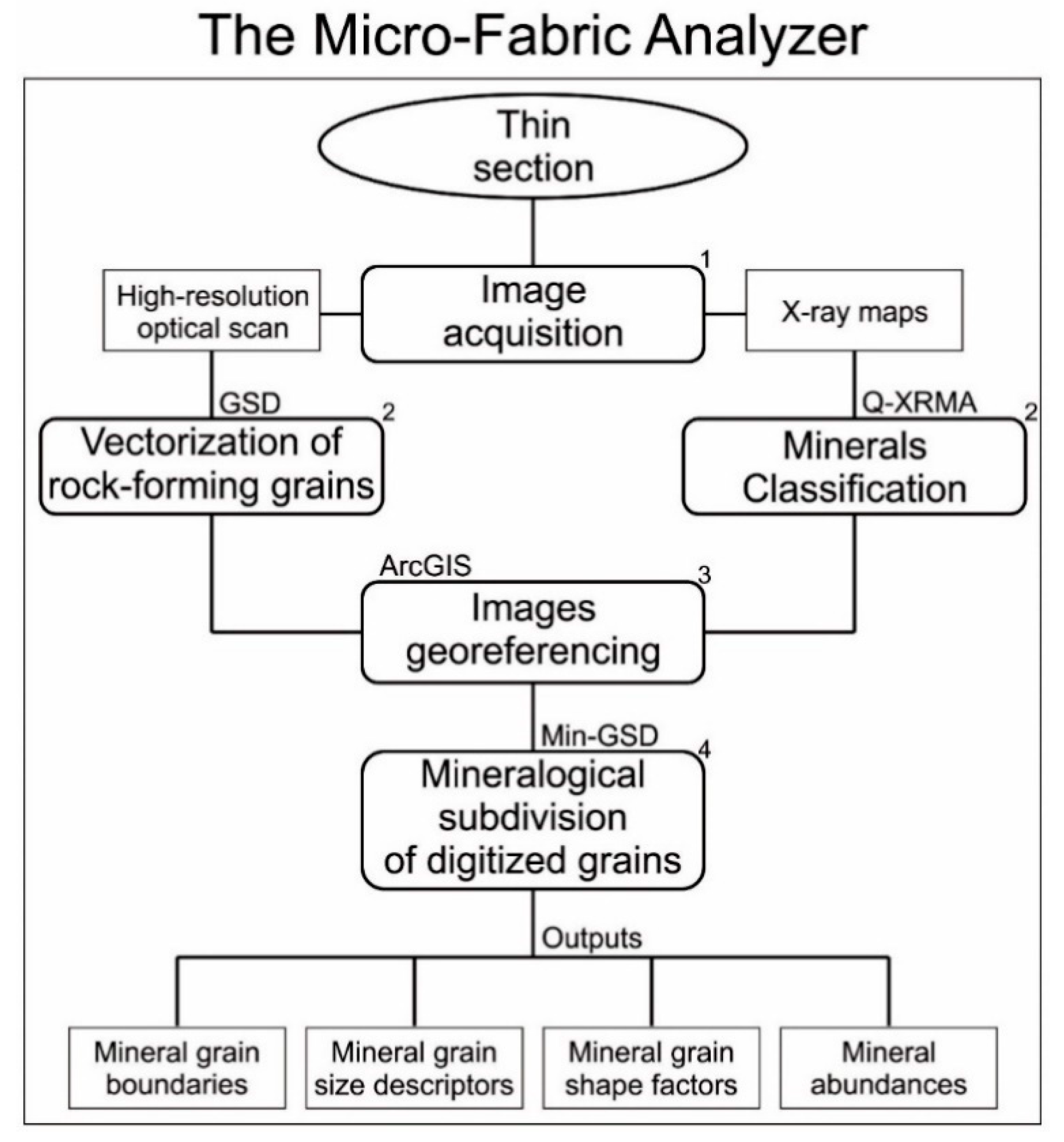
2.2. The Micro-Fabric Analyzer Toolbox: Grain Size Detector (GSD) Tool

The GSD has a simple graphical interface (Figure 2), and it requires a single high-resolution optical input image (Figure 3a,b). The tool consists of five main parts:
(i)
The data storage management through the creation of directories where the outputs will be stored. In this case, the tool prompts the user to specify both the name of the analyzed sample and the path where the output folder will be created (Figure 2);
(ii)
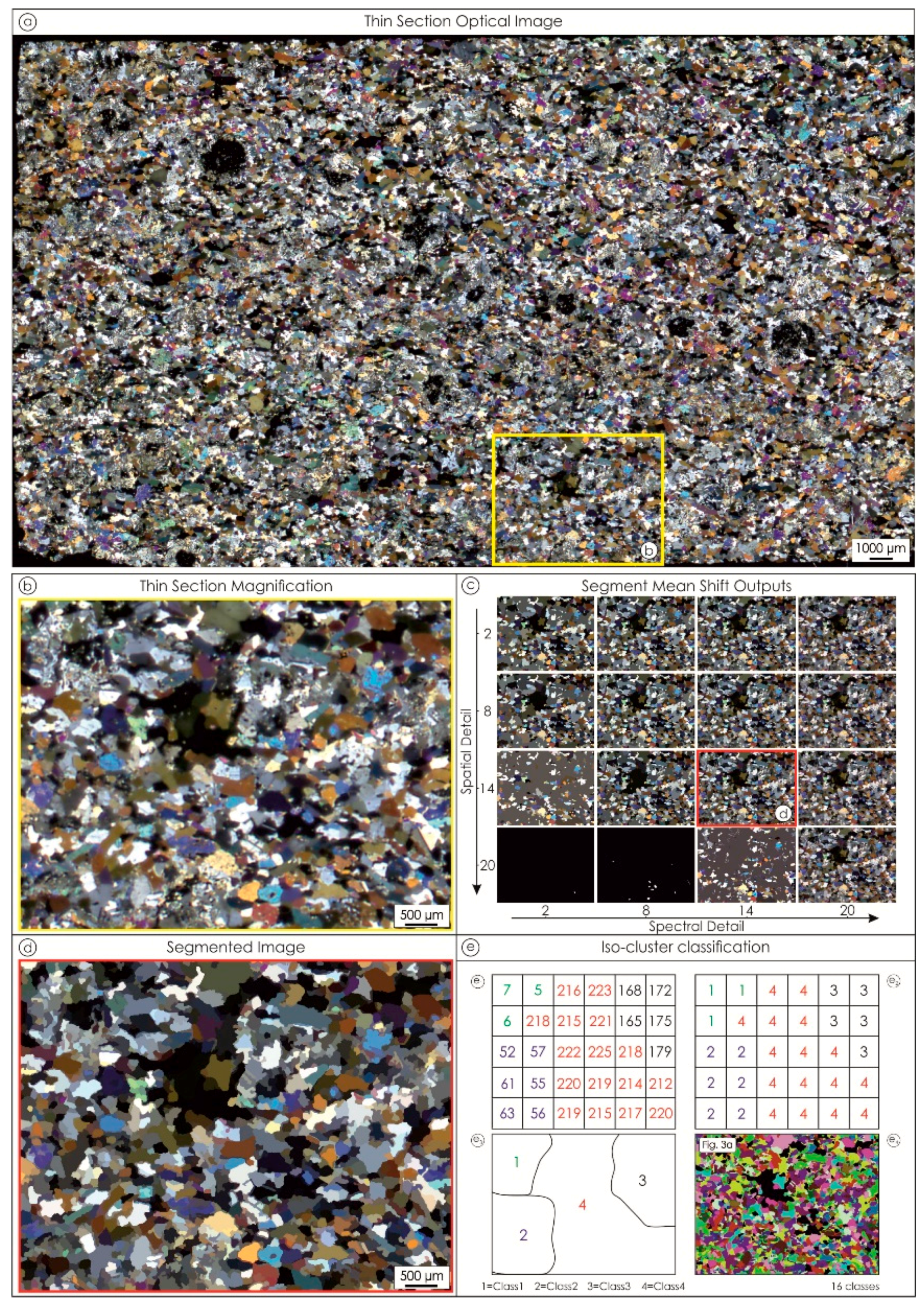
The image segmentation performed by the application of the SMS followed by Iterative self-organization (Iso) cluster classification.
The SMS uses three different parameters named spectral detail, spatial detail, and minimum segment size, to group adjacent pixels having similar colors, and appropriately identify the segments constituting the input image (Figure 2).
The spectral detail (value range: 1.0–20.0) allows the user to separate objects based on color characteristics. A small spectral detail value results in a few segments (Figure 3c), each one covering a large area, and a relatively small number of grains are separated (smoothing effect); instead, a higher spectral detail value results in a higher number of segments and can separate grains having similar color (Figure 3c). The default value is set to 15.5. Nevertheless, the user can control the intensity of spectral smoothing to help obtain features of interest by modifying this value according to the sample studied.
The spatial detail (value range: 1.0–20.0) allows the user to separate objects based on the proximity between features in the input imagery. Opposite to the spectral detail, higher values result in larger segments with a greater smoothing effect, whereas smaller values allow the distinction between small objects clustered together (Figure 3c). The default value is set to 16.0. Similar to spectral detail, the user can control the intensity of spectral smoothing accordingly to the sample investigated.
The minimum segment size gives the minimum size (i.e., area), in pixels, for a group of contiguous pixels to trace a grain. All segments smaller than the specified value will be merged with their best fitting neighbor segment. Smaller values produce less homogeneous segments by preserving color differences due, for instance, to original mineral zoning or twinning, whereas higher values minimize these effects. A value of 200 pixels (corresponding to a grain having an equivalent diameter of ≈85 µm) is set by default in the tool, as it is considered the suitable value to remove artifacts and obtain an optimal segmentation for a thin section scan with a resolution of ≈5 µm of pixel size. Nevertheless, the user can control the minimum size to help obtain features of interest, by modifying this value in the case of samples with small grains.
The iso-cluster classification applies to the SMS output (Figure 3d), allowing finding clusters (i.e., classes) of pixels assigned to specific segments on the basis of the statistical distribution of the pixel color intensities (Figure 3e), computing the minimum Euclidean distance when assigning each pixel to a cluster. In this case, users must define the number of potential clusters (i.e., the maximum number of classes that can result from the clustering process) representative of the segments constituting the input image. Small values are advised to classify rocks with few minerals, whereas a high value is suitable for polymineralic rocks having minerals with different spectral characteristics. The default value is set at 32 classes, but the optimal value depends on the sample, and it is recommended to start by checking the result obtained with a high number, and then to decrease the number of classes if necessary. It is adopted here as a preliminary operation to the subsequent phase of identifying the edges of the segments;
(i)
The edge enhancement by applying gradient e.g., [44] and dilation filters e.g., [7] (Figure 2).
The gradient filter is a type of Sobel edge detection algorithm that calculates the range (i.e., differences between the largest and smallest values) of the pixels in a neighborhood to detect regions that represent edges on an input image by assigning the obtained values to the targeted pixels in a new output image. The gradient filter is useful for identifying contacts between different classes in the classified image (Figure 4a), excluding all the pixels not representing grain boundaries. This condition occurs when the difference between the largest and smallest value of the pixel matrix is equal to zero (Figure 4b). Once the class corresponding to a difference value equal to zero has been obtained, all the others are merged into a single class representing the rough boundaries of the grains (Figure 4c). The GSD allows the user to select the shape and the dimension of the neighborhood area between different options, which are explained in detail in the help menu of the tool (Figure 2). The default neighborhood is a square rectangle with a width and height of three-pixel units, but the user can choose proper values as a function of the investigated sample. Higher values of the pixel units will result in a thickening of the grain boundaries.
The gradient filtering is followed by the application of two rounds of dilation filter. The dilation filter replaces the targeted pixel with the highest value in the neighborhood, and thus, it thickens the grain boundaries (Figure 4d), minimizing the risk of under-segmentation and the occurrence of tiny spurious grains. Analogously to the gradient filter, the default neighborhood is a square rectangle with a width and height of three-pixel units. Each round of dilation filter is followed by a thinning function [55] applied to the rasterized grain boundaries, which reduces the number of pixels representing the width of the boundaries to obtain a linear feature one-pixel wide (Figure 4e);
(i)
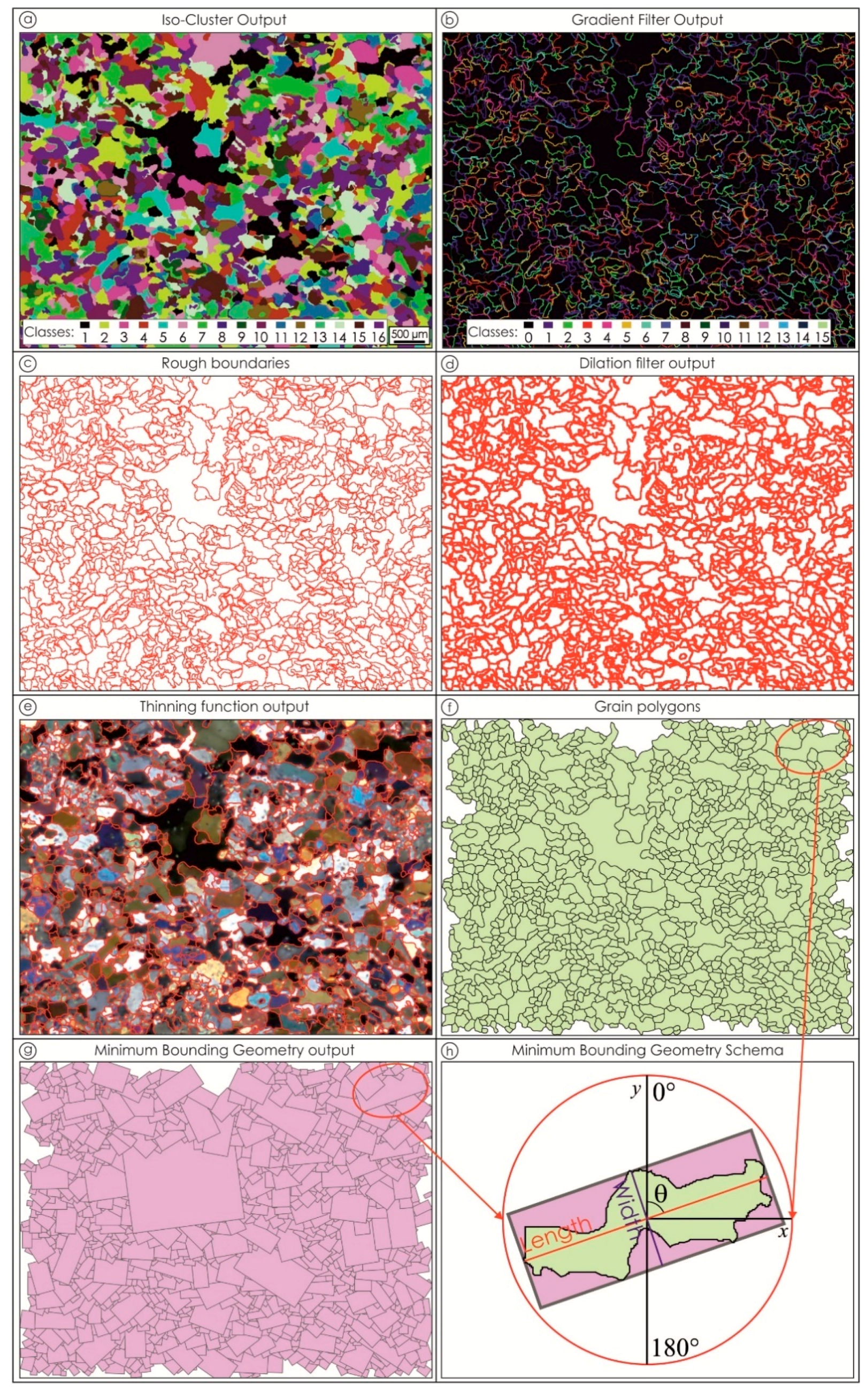
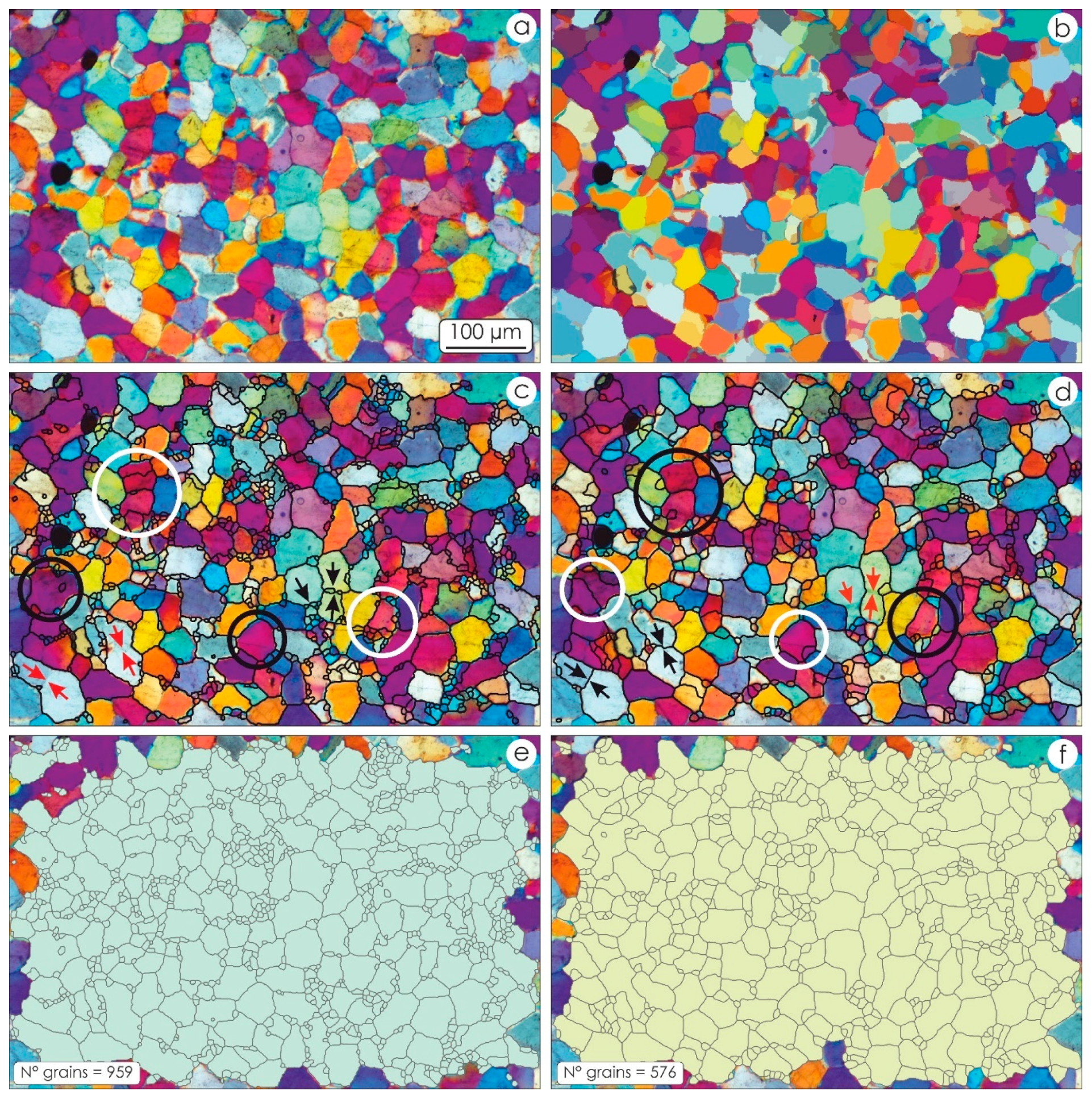
The vectorization step to convert, in vector format (i.e., polylines), the rasterized skeleton of the boundaries. Where the intersections between these polylines form a closed area, polygons (containing attributes regarding their area and perimeter in pixels), representative of rock-forming grains, are automatically digitized. This operation is performed throughout the whole image, obtaining the thin section grains (Figure 4f);
(ii)
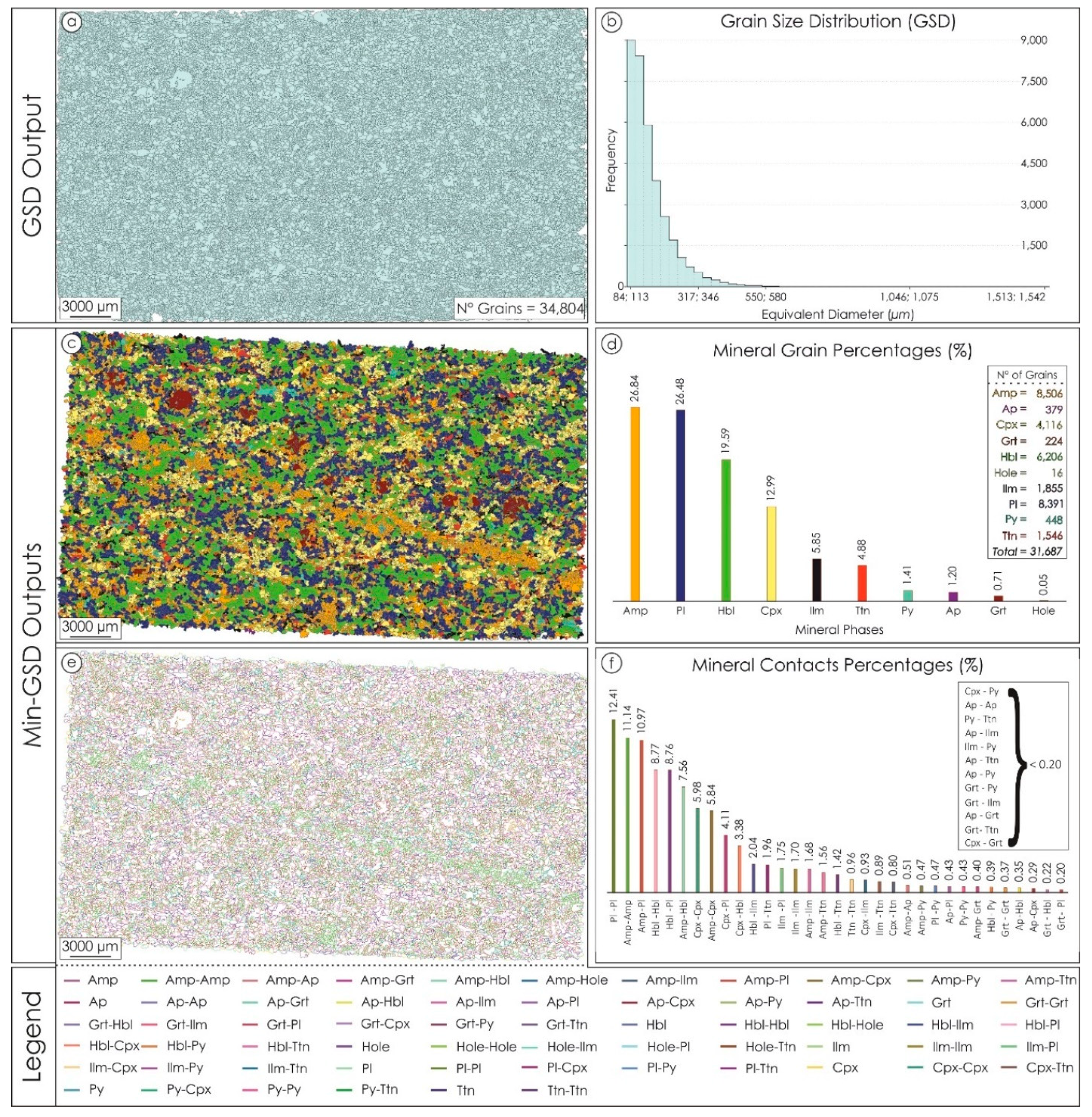
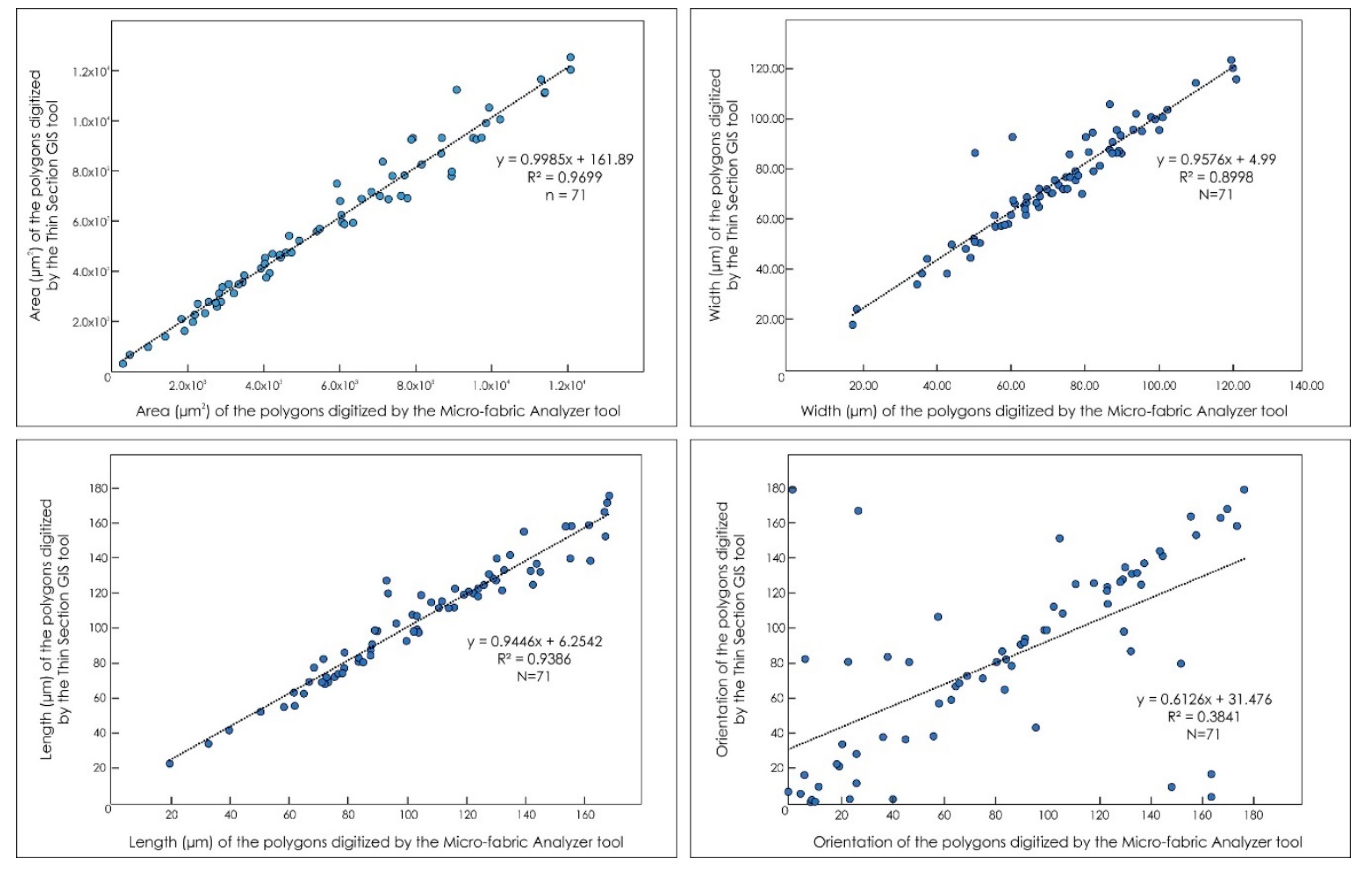
The collection of measurements, by adopting the Minimum Bounding Geometry (MBG) algorithm e.g., [5]. Such a tool creates boxes having the smallest width enclosing each polygon (Figure 4g), in order to collect data about elongation (i.e., length and width axes) and orientation of the grains (Figure 4h). Furthermore, by combining data of the area, perimeter, length, and width of the grains, the tool calculates five fabric parameters more (i.e., aspect ratio, equivalent diameter, roundness, shape factor 1, shape factor 2; Table 2) as defined in the Appendix A. In this case, the tool prompts the user to specify the pixel size of the input image.

2.3. Classification of Rock-Forming Minerals via the Q-XRMA Tool

The Q-XRMA tool [21] is here adopted only to process the element µXRF maps of the entire thin section. In this perspective, we adopted the first analytical cycle of the Q-XRMA, which consists of various stages implying a multivariate statistical data handling of the X-ray maps based on the sequential application of the Principal Components Analysis and the supervised Maximum Likelihood Classification [1]. Such an application allows users to distinguish mineral phases across the analyzed thin section as well as extrapolate the associated modal percentages.

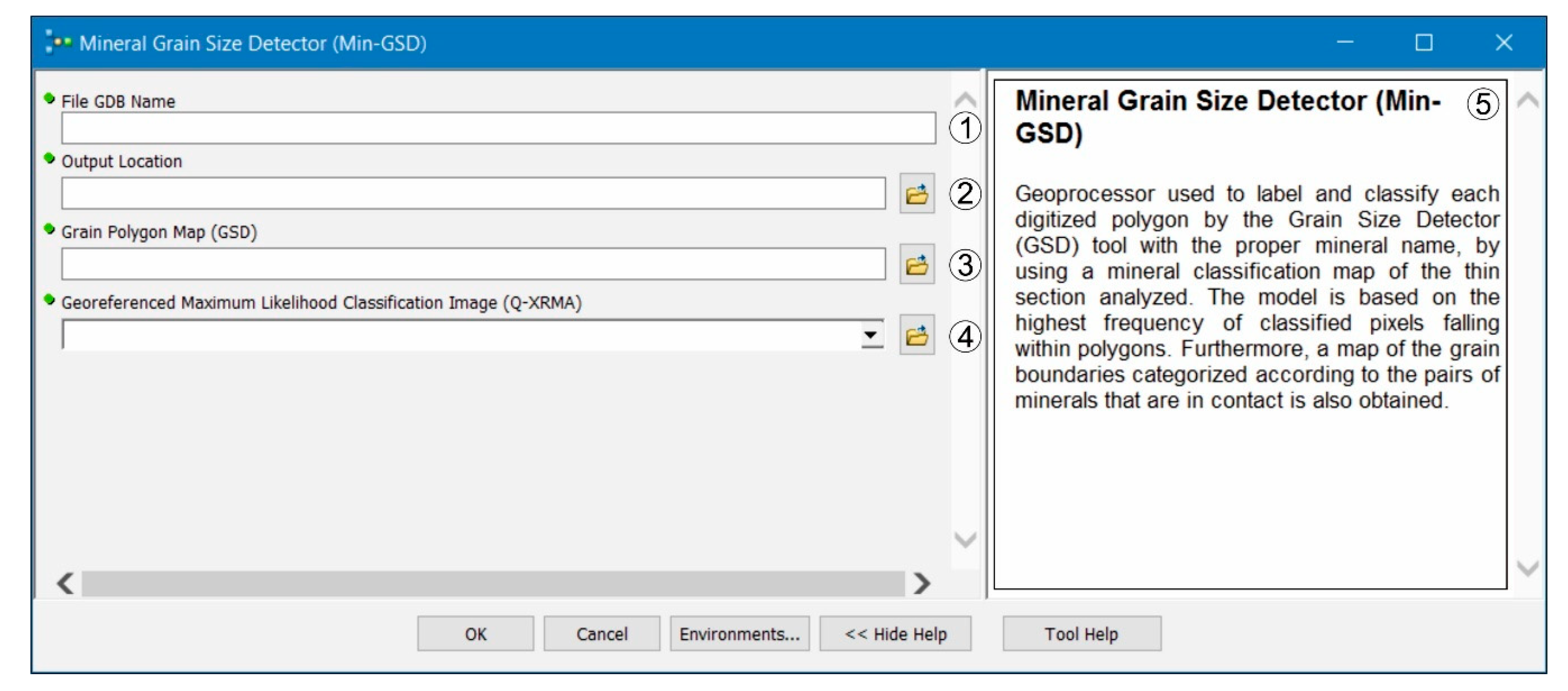
2.4. The Micro-Fabric Analyzer Toolbox: Mineral Grain Size Detector (Min-GSD) Tool

The Min-GSD shows a simple graphical interface (Figure 5) and it allows users to join the output obtained by the GSD (i.e., the map of polygons) with the output of the Q-XRMA (i.e., the map of minerals) to assign to each polygon a specific mineral phase. It requires, as a preliminary operation, a georeferencing step of the mineral classification map and of the thin section scan within the ArcGIS environment (Figure 6a), as these images do not contain specific spatial reference information, as well as they are not perfectly stackable because of the different resolution. In this case, it is necessary to use accurate location data to align the raster data of the map of minerals to the thin section coordinate system, to achieve a reliable overlap between the two images.
The tool consists of four main parts:
(i)
The data storage management. Analogous to the GSD, the tool asks the user to specify both the name of the analyzed sample and the path where the output folder will be created;
(ii)
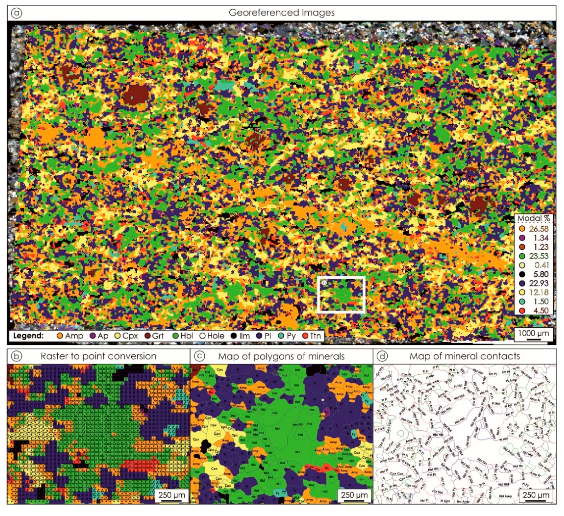
A raster to vector conversion applied to the map of classified minerals, in which a point feature is created at the center of each pixel (Figure 6b). Each point preserves (as an attribute) the mineral phase of the parent pixel in the classified map;
(iii)
The join, based on the spatial relationships, between the attributes of the map of polygons obtained through the GSD tool and the points storing the mineral phase attribute. With this operation, the tool appends, through the “Contains Clementini” function [57], the mineral phase attribute to the attributes of the map of polygons, with the exception that if the join feature (i.e., the points) is entirely on the boundary (no part is properly inside or outside) of the target feature (i.e., the polygons), the feature will not be matched. The “Contain Clementini” function defines the boundary of the polygon as the line separating inside and outside, the boundary of a line is defined as its endpoints, and the boundary of a point is always empty. To ensure a reliable assignment of the mineral attribute to the polygon, the tool calculates the most frequent mineral phase attribute among the points enclosed within each polygon. When it is impossible to determine the most frequent mineral phase attribute among the points enclosed within a given polygon, this will not be assigned to any mineral phase, and it will not be kept in the final output. This step allows users to obtain the map of grains subdivided per mineral phase (Figure 6c) and quantify texture characteristics for single mineral phases (Table 3);
(iv)
The vectorization step to derive a map of grain boundaries, where each boundary maintains information about the contact between a specific couple of minerals (Figure 6d).

3. Results

An amphibolite (Figure 4a and Figure 7), a mylonitic paragneiss (Figure 8), and mylonitic tonalite (Figure 9) are analyzed with the Micro-Fabric Analyzer, to evaluate the potential and limits of the tool and its effectiveness, when coarse-medium grained and relatively fine-grained metamorphic rocks are investigated.
To assess the validity of the tool, a comparison between the results obtained on a sandstone sample by the MFA and the ArcGIS-based Thin Section GIS tool developed by [4], is presented.

3.1. Amphibolite

The selected amphibolite sample is made up of garnet, amphibole, clinopyroxene, plagioclase, pyrite, ilmenite, and titanite mineral phases (Figure 6a), which show different spectral characteristics and variable grain sizes from small (<100 µm) to large (>1000 µm) crystals. Garnet and clinopyroxene show well-shaped large crystals ranging from 500 to 1500 µm in size, whereas amphibole and plagioclase can be found both as large grains and smaller ones grown up as symplectite on garnet.
We applied the GSD by using values of 14, 12, and 200 (Table 4), respectively, for the spectral detail, spatial detail, and minimum segment size. In this way, the tool is able to recognize grains having an equivalent sphere diameter at least greater than 84 µm, incorporating the grains below the detection limit in the surrounding ones. This choice pushed us toward a better segmentation of the input image, selecting a trio of parameters of the SMS that highlights the separation between the various segments, reducing noise and smoothing effects, and minimizing the risk of an over-segmentation. The default value was selected for the iso-cluster classification (Table 4), which resulted in good discrimination between minerals, since no homogenizations between different grains in contact with similar spectral characteristics nor spurious segmentations within the same individual were observed. The GSD permitted digitizing 34,804 grains (Figure 7a) showing a grain size distribution ranging from 84 to 1542 µm (Figure 7b) on the basis of the equivalent diameter (DEQU, see Supplementary Materials). The ≈95% of the sample (i.e., 32,856 polygons) consists of grains having a size between 84 and 300 µm (Figure 7b), whereas the remaining 5% (i.e., 1948 polygons) is made up of grains with a size higher than 300 µm. Despite being few in number, the largest grains (DEQU > 300 µm) cover an area equal to 25% (i.e., 224 mm2) of the investigated sample.
Results obtained by the Min-GSD (Figure 7c) permitted us to classify 31,687 mineral grains predominantly given by brown amphibole (i.e., 8506 polygons), plagioclase (i.e., 8391 polygons), and hornblende (i.e., 6206 polygons), constituting a total modal amount of ≈73% (Figure 7d), which is typical of an amphibolite. Other major mineral constituents are clinopyroxene (i.e., 4116 polygons; ≈13% of the sample) and, to a lesser extent (≈5% of the sample), ilmenite (i.e., 1855 polygons) and titanite (i.e., 1546 polygons), whereas minor constituents (less than 1.5% of modal amount) are given by pyrite (i.e., 448 polygons), apatite (i.e., 379 polygons), and garnet (i.e., 224 polygons) (Figure 7d). The contact map between mineral pairs (Figure 7e) shows that the majority occurs between the same mineralogical phase (e.g., pl-pl, and amp-amp, Figure 7f), and to a lesser extent between amphiboles and plagioclases, amphiboles and pyroxenes, and plagioclases and pyroxenes, while minor mineral pairs make up less than 2% of total contacts (Figure 7f).
As a final result of the entire “Micro-Fabric Analyzer” procedure, a complete quantitative description of the investigated thin section in terms of grain size distribution (Figure 7b), mineral modal abundances (Figure 6a), mineral grain percentages (Figure 7d), and mineral contacts percentage (Figure 7f) is obtained e.g., [47].

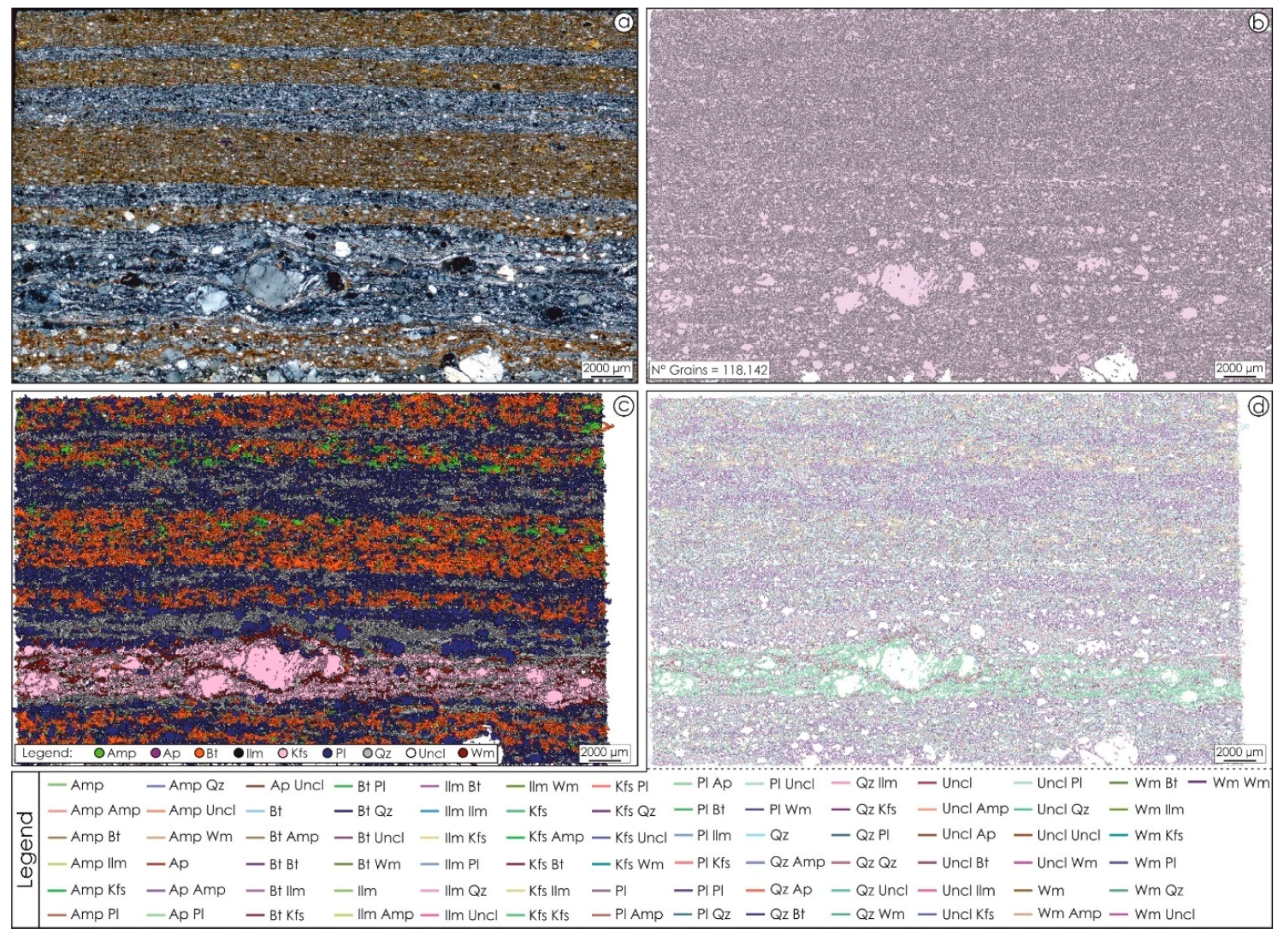
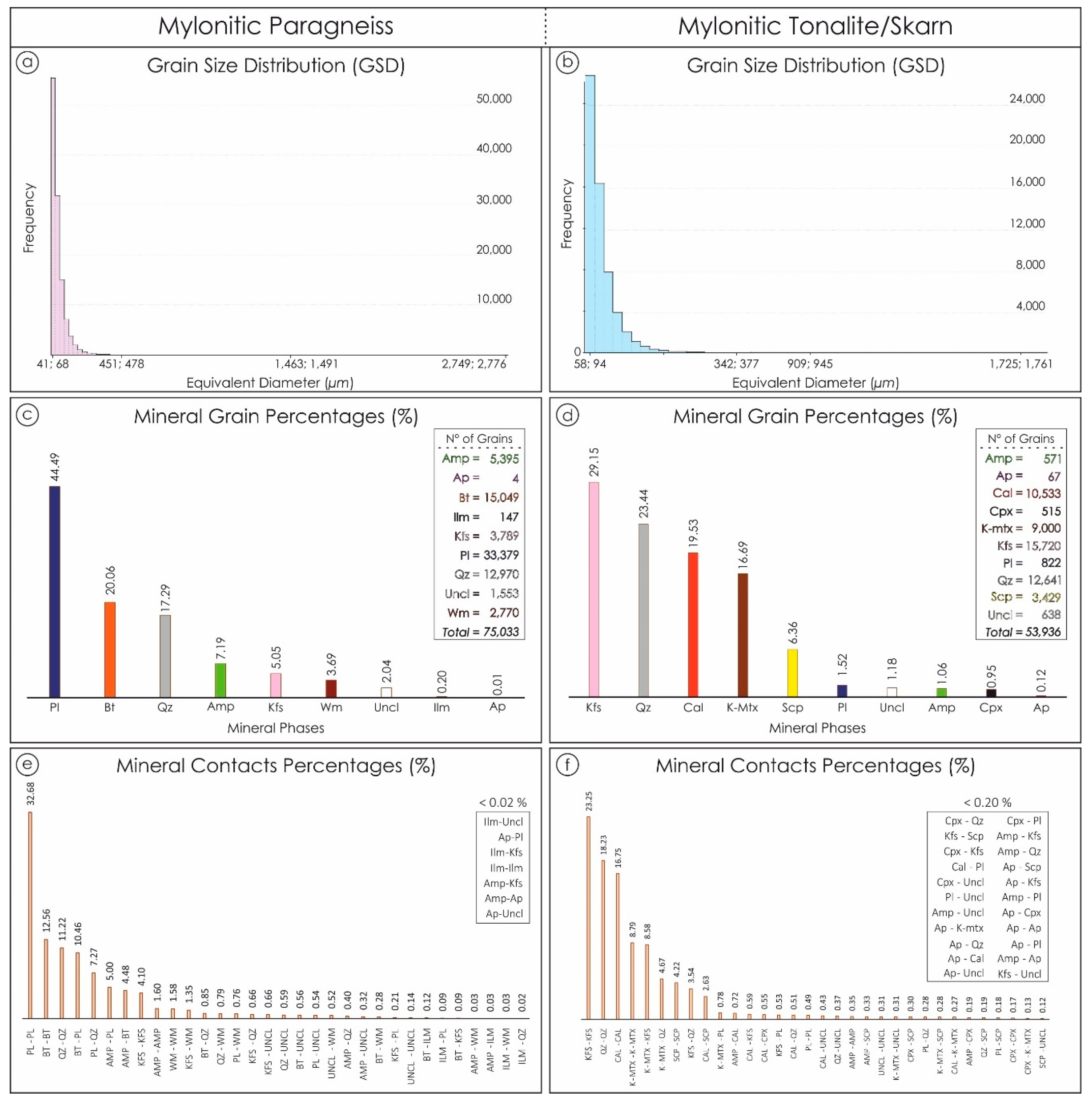
3.2. Mylonitic Paragneiss

The mylonitic paragneiss sample (Figure 8a) has a mineralogical assemblage given by quartz, K-feldspar, plagioclase, biotite, amphibole, and white mica (Figure 8c). The sample is characterized by a pre-shear migmatitic layer testified by quartz-feldspar layers alternating with microcrystalline biotite, which is in association with intensely fractured amphibole crystals. Quartz is constituted by small grain (<50 µm) and tiny amounts of cryptocrystalline quartz infill fractures within K-feldspar and plagioclase porphyroclasts, whereas white mica is also present as tiny crystals within the quartz-feldspar levels.
Since the intense deformation underwent by the sample and the numerous presences of fractures affecting the largest clasts, values of 15, 18, and 50 (Table 4), respectively for the spectral detail, spatial detail, and minimum segment size were selected to obtain performing segmentation results. The spectral detail selected allowed us to maintain high discrimination between large grains, whereas the high spatial detail allowed us to homogenize fractures, inclusions, and zonings affecting porphyroclasts. The minimum segment size fixed the grain detection limit at ≈40 µm in terms of equivalent sphere diameter. This choice can lead to the digitization of spurious grains especially in the case of samples characterized by small grains, but, at the same time, it can be useful to avoid under-segmentation phenomena that would prevent the correct detection of the grain boundary of the larger grains, with consequent overestimation of their actual size. Sixteen classes were selected for the iso-cluster classification (Table 4).
The GSD permitted digitizing 118,142 grains (Figure 8b) showing a grain size distribution ranging from 41 to 2776 µm (Figure 10a). Almost the entire sample (i.e., ≈97%) consists of grains (i.e., 115,001 polygons) having a size between 41 and 200 µm (Figure 10a), whereas the remaining 3% (i.e., 3141 polygons) is made up of grains with a size higher than 200 µm. Despite the low percentage, grains with a DEQU > 200 µm cover an area equal to 24% (i.e., 208 mm2) of the investigated sample.
Results obtained by the Min-GSD (Figure 8c) permitted us to classify 75,033 mineral grains (Figure 10c) with a predominance of plagioclase (i.e., 33,379 polygons), biotite (i.e., 15,049 polygons), and quartz (i.e., 12,970 polygons), constituting a total modal amount of ≈82% (Figure 10c). Other major mineral constituents are amphibole (i.e., 5395 polygons; 7.19% of the sample), K-feldspar (i.e., 3789 polygons; 5.05% of the sample), and to a lesser extent, white mica (i.e., 2770 polygons; 3.69% of the sample). Rare (less than 0.2% of the modal amount) ilmenite (i.e., 147 polygons) and apatite (i.e., four polygons) (Figure 10c) can be observed. The map of pairs of mineral contact (Figure 8d) shows that ≈33% of the grain boundaries is constituted by the contact between plagioclase grains (Figure 10e). High contact percentages are found also between biotite, quartz, amphibole, and K-feldspar.

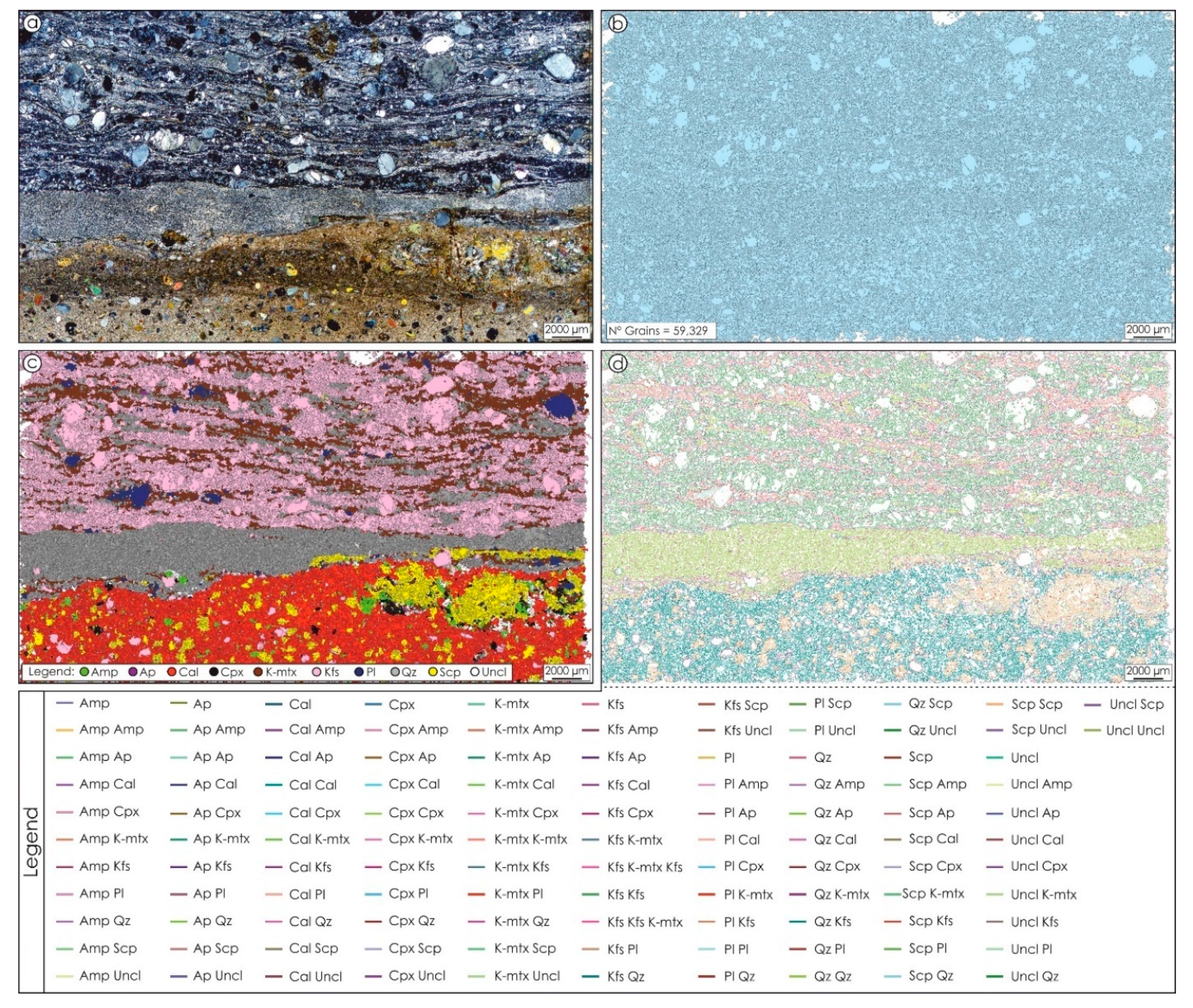
3.3. Mylonitic Tonalite

The mylonitic tonalite (Figure 9a) is constituted by a mineralogical assemblage made up of quartz, K-feldspar, and plagioclase wrapped by a microcrystalline matrix (Figure 9c). Quartz grains develop various ribbon-like structures often interrupted by several systems of fractures. Plagioclase and K-feldspar are present both as porphyroclasts and tiny grains, showing frequent deformation twins and intense fracturing. The tonalite sample (top of Figure 9a) also shows a sharp contact with a mylonitic skarn (bottom of Figure 9a) marked by a layer of cryptocrystalline quartz. The skarn is constituted, mainly, by an association of calcite, K-feldspar, and quartz, which is accompanied by subordinate scapolite, amphibole, and clinopyroxene. Calcite is the most abundant mineral observable in the matrix as cryptocrystalline grains (<50 µm).
In order to digitize properly both small and large rock-forming grains, we selected values of 15, 19, and 100 (Table 4), respectively, for the spectral detail, spatial detail, and minimum segment size, while sixteen classes were adopted for the iso-cluster classification (Table 4).
The GSD results permitted us to identify 59,329 grains (Figure 9b) having a grain size distribution ranging from 58 to 1761 µm (Figure 10b). Analogously to the mylonitic paragneiss, the 92% sample is constituted by tiny grains (i.e., 54,617 polygons) having a size between 58 and 200 µm (Figure 10b). The remnant 8% of the sample (i.e., 4712 polygons) is made up of grains with a size higher than 200 µm and covering an area of 39% (i.e., ≈326 mm2) of the investigated sample.
The Min-GSD (Figure 9c) labeled 53,936 mineral grains (Figure 10d), highlighting K-feldspar mica (i.e., 15,720 polygons; ≈29% of the sample), quartz (i.e., 12,641 polygons; ≈23% of the sample), and the potassium-rich matrix (i.e., 9000 polygons; ≈17% of the sample) as the most abundant minerals characterizing the tonalite. The skarn is mainly composed of calcite (i.e., 10,533 polygons; ≈20% of the sample) and scapolite (i.e., 3429 polygons; ≈6% of the sample), with minor amphibole (i.e., 571 polygons) and clinopyroxene (i.e., 515 polygons) constituting less than 2% of the sample (Figure 10d). Figure 9d shows that the most frequent contacts between minerals occur between the same main mineralogical phase (e.g., kfs-kfs, qz-qz, cal-cal, Figure 10f).

3.4. Quartzarenite

A sandstone sample (Figure 11a) used by [4] to develop an ArcGIS-based edge detector (i.e., Thin Section GIS.tbx—TSG), was here processed through the MFA with the aim to make a comparison between the obtained results with the two different tools. Ref. [4] have addressed the question of the construction of mineral grain size distribution maps by developing a tool that requires three different-oriented optical input images of the same thin section to detect grain boundaries. Such a choice permitted the authors to enhance the recognition of the edges between neighboring grains that could have the same crystallographic orientations. We decided to compare the MFA with the TSG, since both were developed in the ArcGIS environment, allowing quick comparison of the results obtained in terms of edge detection and grain quantification, with the difference that the MFA requires only one input image. In addition, both tools use the same gradient and dilation filters to reduce noise in the input images for improving the recognition of the grain boundaries and the same algorithms to digitize the polygons representative of the rock grains.
The sample investigated show quartz crystals with sharp contact and, in rare cases, an undulate extinction, which could affect the grain boundary detection with the consequent digitization of spurious sub-grains. With the intent to limit this potential hindrance, we selected 14, 6, and 100, respectively for the spectral detail, spatial detail, and minimum segment size. In this case, the low value of the spatial detail permitted high differentiation between neighboring grains showing similar colors (Figure 11b), minimizing an under-segmentation of the image that would result by using a higher value. The comparison between the edge detection obtained by the TSG (Figure 10c) and MFA (Figure 10d) shows pieces of evidence of over- (white circle in Figure 11c,d) and under-segmentation (red arrows in Figure 11c,d) in both tools. If we consider the same regions in the input image where such segmentation issues occur, both tools show, in some cases, more performing results than each other (black circle and arrows in Figure 11c,d). The results obtained by TSG are more segmented with the consequent digitization of a greater number of spurious grains (959 grains, Figure 11e) than the result obtained with MFA (576 grains, Figure 11f), while the influence of under-segmentation affects the results of both instruments in a similar way. We focused and selected those grains with no segmentation errors to make data comparisons in terms of grain sizes and orientations (Figure 12).
We compared the areas, the lengths of the long and short axes, and the orientations (Figure 12) derived from the TSG and the MFA on the same grain. We have found close relationships for the grain area (R2 ≈ 0.99), the length of the short axes (R2 ≈ 0.96), and the length of the long axes (R2 ≈ 0.94) between the polygons digitized by the two different tools, whereas the orientation of the grain derived by the MFA shows differences with respect the TSG-digitized polygons (R2 ≈ 0.61). This is due to small differences in the grain shape obtained by the MFA that influence the creation of the boxes by the MBG algorithm.

4. Discussion

Image processing of thin section scans or micrographs has proven to be a powerful tool for the quantitative extrapolation of rock microstructural features in different fields of geosciences e.g., [1,4,6,31,33,34,49,58,59,60,61]. Using optical thin section images for the grain boundary detection revealed to be more efficient for identifying the edges of the individual grains characterizing rock fabrics, with respect to the image analysis performed starting from mineral physical–chemical properties (e.g., backscattered electron images, X-ray maps, or X-ray tomography) where the shared boundary of two grains of the same mineral species is always indistinguishable. This is partly true, using a single optical input image. In this case, indeed, the grain boundaries between two equal mineral species disappear from sight when the minerals also share the same crystallographic orientation. Automated edge detection techniques require, as a fundamental step, the segmentation of the native optical image. Common issues in applying the segmentation process could be the creation of false grains (i.e., over-segmentation) where fractures, undulate extinctions, or zonings occur, or the disappearance of some grains (under-segmentation) at the contact between two clasts (e.g., red arrows in Figure 11f) displaying a similar birefringence color [44] or if they are smaller than the detection limit dictated by the resolution of the starting image.
When using the “Micro-Fabric Analyzer”, an under-segmentation (i.e., missing grain boundaries) can occur due to the use of an input RGB image acquired at a single orientation of the polarizers, and it is more frequent if low and high values are selected, respectively, for the spectral and spatial detail parameters of the SMS algorithm. In contrast, an over-segmentation (i.e., false grain boundaries) is promoted when high and low values are chosen, respectively, for the spectral and spatial detail, or a low value of the minimum segment size is selected. Despite these potential hindrances, the use of the GIS strengthens the method, which could imply a somewhat higher amount of manual editing at the end of the segmentation step.
An appropriate combination of the tool parameters can minimize the segmentation issues, but the usual complexity of a rock texture implies that a manual editing session is typically necessary to correct for under- and/or over-segmentation. The GIS environment is especially suited for the editing of vectors and can allow for a relatively easy correction of the segmentation issues e.g., [6,44]. The GIS environment is also ideal to query the vector-based maps of the rock texture on the basis of the grain attributes, and this capability can be used to obtain enhanced visualizations of the micro-structural characteristics, which are capable of showing patterns that cannot be recognized through the standard observation of a thin section e.g., [44]. The georeferencing of the map of classified minerals with respect to the original thin section scan is another possible source of error and depends on the operator’s ability to overlay the two images. However, georeferencing maps is a basic operation in GIS, and this issue can be easily overcome as the practice increases. Finally, this method has the advantage of providing a detailed measurement of a very large number of grains in a short time if compared to hand tracing.
Results obtained by using thin section optical scans with a pixel size of ≈5 µm of three rock samples constituted by mineral with different grain sizes highlighted how the MFA is able to digitize fairly accurately large polygons (DEQU > 200 µm). Smaller polygons can be digitized as well, but they increase the chance of running into fake grain creations that would require more post-processing editing. The comparison between the TSG tool developed by [4], which uses three input images of the same region from a thin section, and the MFA shows very similar results in terms of edge detection and grain size (Figure 11). In particular, the possibility of properly setting the parameters of the segmentation algorithms of the MFA according to the sample investigated allows us to obtain more performing results by minimizing possible over-segmentation phenomena (Figure 11d). The grain parameters quantified by the TSG and MFA show close relationships to each other (R2 ≈ 0.9) except for the grain orientation (R2 ≈ 0.6), which results in the parameter being more susceptible to small changes in the digitized grain boundary.
Automatic or semi-automatic methods such as the Micro-Fabric Analyzer toolbox open new perspectives in the quantitative analysis of rock texture. This tool allows the user to obtain from the investigated samples some numerical information that can be displayed as derivative maps (Figure 7 and Figure 10). The large number of the derived fabric parameters (e.g., Table 2 and Supplementary Materials) permits detailed microscopic characterization of the sample thanks to a microscopic information system e.g., [6] in which each detected grain is accompanied by dimensional, geometrical, and compositional data structured in a database (Table 2 and Table 3 and Supplementary Materials). Preliminary versions of the tools embedded in the Micro-Fabric Analyzer toolbox have been already successfully applied in several works. The GSD has revealed to be a valuable asset to conduct vorticity analysis and strain rate estimation on mylonites [53], to integrate microtomography investigations in the reconstruction of the geological evolution of metamorphic rocks [62], and to improve the characterization of plutonic rocks by describing specific textural features such as a potential fabric anisotropy [63]. These applications provide only an idea of the new perspectives opened in the quantitative analysis of rock texture by automatic or semi-automatic methods such as the Micro-Fabric Analyzer toolbox. Furthermore, the integration of a mineralogical distribution map of an entire thin section derived from the classification of µ-XRF elemental maps enhances significantly the mineral phase recognition. The Min-GSD tool allows the automatic attribution of a mineral phase to each polygon grain in a statistically meaningful way (Figure 6), avoiding a manual mineral phase assignment e.g., [6]. This step is also crucial in quantifying the type and the frequency of contacts between minerals (Figure 7e,f, Figure 8d, Figure 9d, and Figure 10e,f), which influence mineral reactions and grain boundary diffusion. This last development opens up the possibility to investigate in a more appropriate way the solid-state reaction progress in metamorphic rocks as well as in ceramics and mortars e.g., [39,64].

5. Conclusions

We presented a new GIS-based procedure for the semi-automatic analysis of a rock thin section micro-structure. The procedure was created with the Model Builder visual programming language embedded in ArcGIS® and is available as a Toolbox extension (Micro-Fabric Analyzer.tbx) as supplementary material. The toolbox, starting from transmitted light images acquired under crossed polarizers and micro-X-ray maps, allows grain boundary detection, mineral classification, texture characterization, and modal analysis. The toolbox can help users extract quantitative information from rocks through better quantification of the fabric parameters useful to describe different evolutionary stages of a given rock, whose features often derive from counterbalancing factors controlled by mineral crystallization, mineral reaction, grain boundary diffusion, deformation, etc.
As final remarks, we can summarize the following: (i) the toolbox constitutes a simple and a relatively fast means to derive the microstructural information of a rock if compared to a hand-tracing procedure; (ii) the Segment Mean Shift algorithm used in the GSD segmentation tool can be tuned to fit the characteristics of different rocks, and the application of a specific sequence of gradient, dilation, and thin functions improves the output reducing artifacts from the segmented image; (iii) each grain polygon is issued with a thorough set of measurements (size descriptors and shape factors) stored as attributes, and they can be easily located within the reference frame of the thin section; (iv) comparison with existing methods shows similar results in terms of edge detection and quantification of the grain parameters; (v) the grain orientation derived by the MFA is most affected by changes in the digitized polygon shape; (vi) on the basis of the georeferencing of the mineral classification map and the original thin section scan, the Min-GSD package allows an automatic statistically meaningful labeling of each polygon with a mineral phase, without the need for manual mineral identification; (vii) the entire procedure takes full advantage of GIS in terms of management and visualization of the derived data, which are stored in an easily queryable database. The use of GIS allows easy editing of vectors to correct issues in the segmentation process, enhanced visualization of the fabric as colored maps, and the straightforward generation of plots illustrating the texture characteristics of the sample.

Supplementary Materials

The following are available online at https://0-www-mdpi-com.brum.beds.ac.uk/2220-9964/10/2/51/s1, Micro-Fabric Analyzer (S1).

Author Contributions

Conceptualization: Roberto Visalli, Gaetano Ortolano; Methodology: Roberto Visalli, Gaetano Ortolano; Software: Roberto Visalli; Validation: Roberto Visalli, Gaston Godard, Gaetano Ortolano; Formal Analysis: Roberto Visalli, Gaston Godard, Gaetano Ortolano; Investigation: Roberto Visalli; Resources: Gaetano Ortolano, Rosolino Cirrincione; Data Curation; Roberto Visalli; Writing—Original Draft Preparation: Roberto Visalli, Gaetano Ortolano, Gaston Godard; Writing—Review and Editing: Roberto Visalli, Gaetano Ortolano, Gaston Godard; Figure editing: Roberto Visalli; Supervision; Gaetano Ortolano, Rosolino Cirrincione; Project Administration: Rosolino Cirrincione, Funding Acquisition: Gaetano Ortolano, Rosolino Cirrincione All authors have read and agreed to the published version of the manuscript.

Funding

This research was funded by University of Catania (PIAno di inCEntivi per la RIcerca di Ateneo 2020/2022—Pia.Ce.Ri), Grant Number: 22722132153, within the project: ”Combined geomatic and petromatic applications: The new frontier of geoscience investigations from field- to micro- scale—(GeoPetroMat)”.

Institutional Review Board Statement

Not applicable.

Informed Consent Statement

Not applicable.

Data Availability Statement

The data presented in this study are available in the supplementary material here and in [4].

Acknowledgments

The authors appreciate very much the former deep review of the original paper made by Simone Tarquini and Renee Heibronner that enhanced significantly the software and data presentation. The authors are grateful to the four anonymous reviewer meticulous reviews, which improved the quality of the original manuscript, and to Kwon Rausis for the editorial handling of the manuscript and thoughtful suggestions.

Conflicts of Interest

The authors declare no conflict of interest.

Appendix A

  • Area (A)
The grain area represents the sum of the areas of all pixels enclosed within a polygon:
A = A s q p x
where A is the area of a specific grain and A s q p x is the total area of the pixels.
As the area must be converted into micrometers, we applied a conversion function that takes into account the pixel size of the thin section:
A   ( µ m 2 ) = pixel   size   ×   A s q p x .
  • Perimeter (P)
The grain perimeter represents the total number of pixels along the grain boundary and it is calculated as follows:
P = P p x .
Similar to the area, the perimeter, P , is converted into micrometers according to the following:
P   ( µ m ) = pixel   size   ×   P p x  
where P p x is the total number of the pixels along the boundary of the digitized grain.
  • Length (L)
The grain length represents the total number of pixels along the long axis of the rectangle obtained through the Minimum Bounding Geometry algorithm, and it is calculated as follows:
L = L p x .
In addition, in this case, the length parameter is converted into micrometers according to the following:
L   ( µ m ) = pixel   size   ×   L p x .
  • Width (W)
The grain width represents the total number of pixels along the short axis of the rectangle obtained through the Minimum Bounding Geometry algorithm, and it is calculated as follows:
W = W p x .
Again, the width parameter is converted into micrometers according to the following:
W   ( µ m ) = pixel   size   ×   W p x .
  • Length Orientation (Clockwise from vertical direction: from 0° to 180°)
The length orientation is the clockwise angle (i.e., the azimuth) between the grain length parameter and the vertical direction, y (see Figure 4h).
  • Aspect Ratio (AsR)
The grain aspect ratio is used for strain analysis, as it grows with increasing strain, from 1 to infinity, and it is calculated as follows:
A s R = L W  
where L and W are respectively the long and short axes of the grain.
  • Equivalent Diameter (DEQU)
The equivalent diameter is the diameter of a circle having the same area as the grain, and it is calculated as follows:
D E Q U = 2 A π   .
  • Roundness (R)
The roundness parameter is the reciprocal of the aspect ratio and limited to values between 0 and 1.
  • Shape Factor 1 (SF1)
The Shape Factor 1 measures the deviation of a given grain from a reference shape, which is here considered the circle. We adopted the formulation of [33], and it is calculated as follows:
S F 1 = P 2 π A   .
This shape factor can assume values between 1 for a circle and ∞ for something infinitely noncircular.
  • Shape Factor 2 (SF2)
Similar to SF1, the Shape Factor 2 measures the deviation of a given grain from a circle, and it is calculated according to [33] as follows:
S F 2 = 4 π A P 2 .
This shape factor assumes values between 1 for a circle and 0 for something infinitely noncircular.

References

  1. Heilbronner, R. Automatic grain boundary detection and grain size analysis using polarization micrographs or orientation images. J. Struct. Geol. 2000, 22, 969–981. [Google Scholar] [CrossRef]
  2. Tarquini, S.; Armienti, P. Quick determination of crystal size distributions of rocks by means of a color scanner. Image Anal. Stereol. 2002, 22, 27–34. [Google Scholar] [CrossRef]
  3. Abràmoff, M.D.; Magalhaes, P.J.; Ram, S.J. Image processing with ImageJ. Biophotonics Int. 2004, 11, 36–42. [Google Scholar]
  4. Li, Y.; Onasch, C.M.; Guo, Y. GIS-based detection of grain boundaries. J. Struct. Geol. 2008, 30, 431–444. [Google Scholar] [CrossRef]
  5. DeVasto, M.A.; Czeck, D.M.; Bhattacharyya, P. Using image analysis and ArcGIS® to improve automatic grain boundary detection and quantify geological images. Comput. Geosci. 2012, 49, 38–45. [Google Scholar] [CrossRef]
  6. Tarquini, S.; Favalli, M. A microscopic information system (MIS) for petrographic analysis. Comput. Geosci. 2010, 36, 665–674. [Google Scholar] [CrossRef] [Green Version]
  7. Heilbronner, R.; Barrett, S. Image Analysis in Earth Sciences, 1st ed.; Springer-Verlag: Berlin/Heidelberg, Germany, 2014. [Google Scholar] [CrossRef]
  8. Baker, D.R.; Mancini, L.; Polacci, M.; Higgins, M.D.; Gualda, G.A.R.; Hill, R.J.; Rivers, M.L. An introduction to the application of X-ray microtomography to the three-dimensional study of igneous rocks. Lithos 2012, 148, 262–276. [Google Scholar] [CrossRef]
  9. Cnudde, V.; Boone, M.N. High-resolution X-ray computed tomography in geosciences: A review of the current technology and applications. Earth-Sci. Rev. 2013, 123, 1–17. [Google Scholar] [CrossRef] [Green Version]
  10. Raneri, S.; Cnudde, V.; De Kock, T.; Derluyn, H.; Barone, G.; Mazzoleni, P. X-ray computed micro-tomography to study the porous structure and degradation processes of a building stone from Sabucina (Sicily). Eur. J. Mineral. 2015, 27, 279–288. [Google Scholar] [CrossRef]
  11. Bloise, A.; Ricchiuti, C.; Lanzafame, G.; Punturo, R. X-ray synchrotron microtomography: A new technique for characterizing chrysotile asbestos. Sci. Total Environ. 2020, 703, 135675. [Google Scholar] [CrossRef]
  12. Borghi, A.; Spiess, R. Studying metamorphic microstructures: A brief insight on modern methodological approaches. Period. Mineral. 2004, 73, 235–247. [Google Scholar]
  13. Liu, J.L.; Cao, S.Y.; Zou, Y.X.; Song, Z.J. EBSD analysis of rock fabrics and its application. Geol. Bull. China 2008, 27, 1638–1645. [Google Scholar]
  14. Prior, D.J.; Mariani, E.; Wheeler, J. EBSD in the Earth Sciences: Applications, Common Practice, and Challenges. In Electron Backscatter Diffraction in Materials Science; Schwartz, A., Kumar, M., Adams, B., Field, D., Eds.; Springer: Boston, MA, USA, 2009. [Google Scholar] [CrossRef]
  15. Panozzo Heilbronner, R.; Pauli, C. Integrated spatial and orientation analysis of quartz c-axes by computer-aided microscopy. J. Struct. Geol. 1993, 15, 369–382. [Google Scholar] [CrossRef]
  16. Stöckhert, B.; Duyster, J. Discontinuous grain growth in recrystallised vein quartz-implications for grain boundary structure, grain boundary mobility, crystallographic preferred orientation, and stress history. J. Struct. Geol. 1999, 21, 1477–1490. [Google Scholar] [CrossRef]
  17. Fueten, F.; Goodchild, J.S. Quartz c-axes orientation determination using the rotating polarizer microscope. J. Struct. Geol. 2001, 23, 895–902. [Google Scholar] [CrossRef]
  18. Hassanpour, R. The use of ArcGIS for determination of quartz optical axis orientation in thin section images. J. Microsc. 2012, 245, 276–287. [Google Scholar] [CrossRef]
  19. Bachmann, F.; Hielscher, R.; Schaeben, H. Grain detection from 2d and 3d EBSD data-Specification of the MTEX algorithm. Ultramicroscopy 2011, 111, 1720–1733. [Google Scholar] [CrossRef]
  20. Ortolano, G.; Zappalà, L.; Mazzoleni, P. X-ray Map Analyzer: A new ArcGIS® based tool for the quantitative statistical data handling of X-ray maps (Geo- and material-science applications). Comput. Geosci. 2014, 72, 49–64. [Google Scholar] [CrossRef]
  21. Ortolano, G.; Visalli, R.; Godard, G.; Cirrincione, R. Quantitative X-ray Map Analyser (Q-XRMA): A new GIS-based statistical approach for Mineral Image Analysis. Comput. Geosci. 2018, 115, 56–65. [Google Scholar] [CrossRef]
  22. Cossio, R.; Borghi, A. PETROMAP: MS-DOS software package for quantitative processing of X-ray maps of zoned minerals. Comput. Geosci. 1998, 24, 797–803. [Google Scholar] [CrossRef]
  23. Lanari, P.; Vidal, O.; De Andrade, V.; Dubacq, B.; Lewin, E.; Grosch, E.; Schwartz, S. XMapTools: A MATLAB©-based program for electron microprobe Xray image processing and geothermobarometry. Comput. Geosci. 2014, 62, 227–240. [Google Scholar] [CrossRef] [Green Version]
  24. Tinkham, D.K.; Ghent, E.D. XRMapAnal: A program for analysis of quantitative X-ray maps. Am. Mineral. 2005, 90, 737–744. [Google Scholar] [CrossRef]
  25. Goodchild, J.S.; Fueten, F. Edge detection in petrographic images using the rotating polarizer stage. Comput. Geosci. 1998, 24, 745–751. [Google Scholar] [CrossRef]
  26. Bartozzi, M.; Boyle, A.P.; Prior, D.J. Automated grain boundary detection and classification in orientation contrast images. J. Struct. Geol. 2000, 22, 1569–1579. [Google Scholar] [CrossRef]
  27. McEwan, I.K.; Sheen, T.M.; Cunningham, G.J.; Allen, A.R. Estimating the size composition of sediment surfaces through image analysis. Proc. Inst. Civ. Eng. Water Marit. Energy 2000, 142, 189–195. [Google Scholar] [CrossRef]
  28. Thompson, S.; Fueten, F.; Bockus, D. Mineral identification using artificial neural network and the rotating polarizer stage. Comput. Geosci. 2001, 27, 1081–1089. [Google Scholar] [CrossRef]
  29. Gu, Y. Automated scanning electron microscope based mineral liberation analysis: An introduction to JKMRC/FEI mineral liberation analyser. J. Miner. Mater. Charact. Eng. 2003, 2, 33–41. [Google Scholar] [CrossRef]
  30. Miriello, D.; Crisci, G.M. Image analysis and flatbed scanners. A visual procedure in order to study the macro-porosity of the archaeological and historical mortars. J. Cult. Herit. 2006, 7, 186–192. [Google Scholar] [CrossRef]
  31. Perring, C.S.; Barnes, S.J.; Verrall, M.; Hill, R.E.T. Using automated digital image analysis to provide quantitative petrographic data on olivine-phyric basalts. Comput. Geosci. 2004, 30, 183–195. [Google Scholar] [CrossRef]
  32. Sardini, P.; Moreau, E.; Sammartino, S.; Touchard, G. Primary mineral connectivity of polyphasic igneous rocks by high-quality digitisation and 2D image analysis. Comput. Geosci. 1999, 25, 599–608. [Google Scholar] [CrossRef]
  33. Lexa, O.; Štípská, P.; Schulmann, K.; Baratoux, L.; Kröner, A. Contrasting textural record of two distinct metamorphic events of similar P-T conditions and different durations. J. Metamorph. Geol. 2005, 23, 649–666. [Google Scholar] [CrossRef]
  34. Martìnez-Martìnez, J.; Benavente, D.; Garcìa del Cura, M.A. Petrographic quantification of brecciated rocks by image analysis. Application to the interpretation of elastic wave velocities. Eng. Geol. 2007, 90, 41–54. [Google Scholar] [CrossRef]
  35. Beggan, C.; Hamilton, C.W. New image processing software for analyzing object size-frequency distributions, geometry, orientation, and spatial distribution. Comput. Geosci. 2010, 36, 539–549. [Google Scholar] [CrossRef]
  36. Berger, A.; Herwegh, M.; Schwarzm, J.O.; Putlitz, B. Quantitative analysis of crystal/grain sizes and their distributions in 2D and 3D. J. Struct. Geol. 2010, 33, 1751–1763. [Google Scholar] [CrossRef]
  37. Zucali, M.; Corti, L.; Delleani, F.; Zanoni, D.; Spalla, M.I. 3D reconstruction of fabric and metamorphic domains in a slice of continental crust involved in the Alpine subduction system: The example of Mt. Mucrone (Sesia–Lanzo Zone, Western Alps). Int. J. Earth Sci. 2020, 109, 1337–1354. [Google Scholar] [CrossRef]
  38. Launeau, P.; Cruden, A.R.; Bouchez, J.L. Mineral recognition in digital images of rocks: A new approach using multichannel classification. Can. Mineral. 1994, 32, 919–933. [Google Scholar]
  39. Coutelas, A.; Godard, G.; Blanc, P.; Person, A. Les mortiers hydrauliques: Synthèse bibliographique et premiers résultats sur des mortiers de Gaule romaine. Rev. d’Archéom. 2004, 28, 127–139. [Google Scholar] [CrossRef]
  40. Friel, J.J.; Lyman, C.E. X-ray mapping in electron-beam instruments. Microsc. Microanal. 2006, 12, 2–25. [Google Scholar] [CrossRef] [Green Version]
  41. Mouchi, V.; Crowley, Q.G.; Ubide, T. AERYN: A simple standalone application for visualizing and enhancing elemental maps. Appl. Geochem. 2016, 75, 44–53. [Google Scholar] [CrossRef] [Green Version]
  42. Lanari, P.; Vho, A.; Bovay, T.; Airaghi, L.; Centrella, S. Quantitative compositional mapping of mineral phases by electron probe micro-analyser. Geol. Soc. Lond. Spec. Publ. 2019, 478, 39–63. [Google Scholar] [CrossRef]
  43. Cirrincione, R.; Fazio, E.; Heilbronner, R.; Kern, H.; Mengel, K.; Ortolano, G.; Pezzino, A.; Punturo, R. Microstructure and elastic anisotropy of naturally deformed leucogneiss from a shear zone in Montalto (southern Calabria, Italy). Geol. Soc. Lond. Spec. Publ. 2010, 332, 49–68. [Google Scholar] [CrossRef]
  44. Barraud, J. The use of watershed segmentation and GIS software for textural analysis of thin sections. J. Volcanol. Geotherm. Res. 2006, 154, 17–33. [Google Scholar] [CrossRef]
  45. Kocabas, V.; Dragicevic, S. Enhancing a GIS cellular automata model of land use change: Bayesian networks, influence diagrams and causality. Trans. GIS 2007, 11, 681–702. [Google Scholar] [CrossRef]
  46. Gorsevski, P.V.; Onasch, C.M.; Farver, J.R.; Ye, X. Detecting grain boundaries in deformed rocks using a cellular automata approach. Comput. Geosci. 2012, 42, 136–142. [Google Scholar] [CrossRef]
  47. Ortolano, G.; Visalli, R.; Cirrincione, R.; Rebay, G. PT-path reconstruction via unravelling of peculiar zoning pattern in atoll shaped garnets via image assisted analysis: An example from the Santa Lucia del Mela garnet micaschists (Northeastern Sicily-Italy). Period. Mineral. 2014, 83, 257–297. [Google Scholar] [CrossRef]
  48. Fiannacca, P.; Ortolano, G.; Pagano, M.; Visalli, R.; Cirrincione, R.; Zappalà, L. IG-Mapper: A new ArcGIS® toolbox for the geostatistics-based automated geochemical mapping of igneous rocks. Chem. Geol. 2017, 470, 75–92. [Google Scholar] [CrossRef]
  49. Fazio, E.; Ortolano, G.; Visalli, R.; Cirrincione, R.; Fiannacca, P.; Kern, H.; Mengel, K.; Pezzino, A.; Punturo, R. Strain rates of the syn-tectonic Symvolon pluton (Southern Rhodope Core Complex, Greece): An integrated approach combining quartz paleopiezometry, flow laws and PT pseudosections. Ital. J. Geosci. 2018, 137, 219–237. [Google Scholar] [CrossRef]
  50. Ortolano, G.; Zappala, L. Management and deployment of rock-analysis data from thin section—to field-scale. Rend. Online Soc. Geol. Ital. 2012, 21, 726–728. [Google Scholar] [CrossRef]
  51. Asmussen, P.; Conrad, O.; Günter, A.; Kirsch, M.; Riller, U. Semi-automatic segmentation of petrographic thin section images using a “seeded-region growing algorithm” with as application to characterize weathered subarkose sandstone. Comput. Geosci. 2015, 83, 89–99. [Google Scholar] [CrossRef]
  52. Berrezueta, E.; Domínguez-Cuesta, M.J.; Rodríguez-Rey, Á. Semi-automated procedure of digitalization and study of rock thin section porosity applying optical image analysis tools. Comput. Geosci. 2019, 124, 14–26. [Google Scholar] [CrossRef]
  53. Ortolano, G.; Fazio, E.; Visalli, R.; Alsop, I.G.; Pagano, M.; Cirrincione, R. Quantitative microstructural analysis of mylonites formed during Alpine tectonics in the western Mediterranean realm. J. Struct. Geol. 2020, 131. [Google Scholar] [CrossRef]
  54. Zhang, X.; Liu, B.; Wang, J.; Zhang, Z.; Shi, K.; Wu, S. Adobe photoshop quantification (PSQ) rather than point-counting: A rapid and precise method for quantifying rock textural data and porosities. Comput. Geosci. 2014, 69, 62–71. [Google Scholar] [CrossRef]
  55. Zhan, C. A Hybrid Line Thinning Approach. In Proceedings of the Auto-Carto 11, Minneapolis, MN, USA, 30 October–1 November 1993; pp. 396–405. [Google Scholar]
  56. Whitney, D.L.; Evans, B.W. Abbreviations for names of rock-forming minerals. Am. Mineral. 2010, 95, 185–187. [Google Scholar] [CrossRef]
  57. Clementini, E.; Sharma, J.; Egenhofer, M.J. Modelling topological spatial relations: Strategies for query processing. Comput. Graph. 1994, 18, 815–822. [Google Scholar] [CrossRef]
  58. Caracciolo, L.; Tolosana-Delgado, R.; Le Pera, E.; Von Eynatten, H.; Arribas, J.; Tarquini, S. Influence of granitoid textural parameters on sediment composition: Implications for sediment generation. Sediment. Geol. 2012, 280, 93–107. [Google Scholar] [CrossRef] [Green Version]
  59. Ortolano, G.; Visalli, R.; Fazio, E.; Fiannacca, P.; Godard, G.; Pezzino, A.; Punturo, R.; Sacco, V.; Cirrincione, R. Tectono-metamorphic evolution of the Calabria continental lower crust: The case of the Sila Piccola Massif. Int. J. Earth Sci. 2020, 109, 1295–1319. [Google Scholar] [CrossRef]
  60. Ortolano, G.; D’Agostino, A.; Pagano, M.; Visalli, R.; Zucali, M.; Fazio, E.; Alsop, I.; Cirrincione, R. ArcStereoNet: A new ArcGIS® toolbox for projection and analysis of structural and microstructural data. ISPRS Int. J. Geo.-Inf. 2021, 10. [Google Scholar]
  61. Fazio, E.; Punturo, R.; Fazio, E.; Cirrincione, R.; Ker, H.; Pezzino, A.; Wenk, H.R.; Goswami, S.; Mamtani, M.A. Quartz preferred orientation in naturally deformed mylonitic rocks (Montalto shear zone–Italy): A comparison of results by different techniques, their advantages and limitations. Int. J. Earth Sci. (Geol. Rundsch.) 2017, 106, 2259–2278. [Google Scholar] [CrossRef]
  62. Corti, L.; Zucali, M.; Visalli, R.; Mancini, M.; Sayab, M. Integrating X-Ray computed tomography with chemical imaging to quantify mineral re-crystallization from granulite to eclogite metamorphism in the Western Italian Alps (Sesia-Lanzo Zone). Front. Earth Sci. 2019, 7. [Google Scholar] [CrossRef]
  63. Ortolano, G.; D’Agostino, A.; Visalli, R.; Cirrincione, R. Plutonic rocks classification: A child’s play. Rend. Online Soc. Geol. Ital. 2019, 49, 46–54. [Google Scholar] [CrossRef]
  64. Belfiore, C.M.; Fichera, G.V.; Ortolano, G.; Pezzino, A.; Visalli, R.; Zappalà, L. Image processing of the pozzolanic reactions in Roman mortars via X-ray Map Analyser. Microchem. J. 2016, 125, 242–253. [Google Scholar] [CrossRef]
Figure 1. The workflow of the Micro-Fabric Analyzer.
Ijgi 10 00051 g001
Figure 2. ArcGIS® Graphical User Interface of the Grain Size Detector (GSD) tool: (1) the data storage management settings; (2) the image segmentation settings; (3) the edge enhancement settings; (4) the units of measure of the input image to be set for collecting measurements of grain data; (5) the help menu of the tool showing hints about the required inputs. Green circles on the left side mark mandatory inputs.
Ijgi 10 00051 g002
Figure 3. GSD tool segmentation steps: (a) the thin section optical image (39.1 × 23.1 mm2 in size with a pixel size of 5.29 µm). Inset represents Figure 3b; (b) magnification of the thin section; (c) the outputs of the Segment Mean Shift algorithm at different settings of spatial and spectral detail parameters; (d) the segmented image obtained with values of 14 for both spatial and spectral details; (e) (e1e3) schematization of the iso-cluster classification by choosing four classes: (e1) the pixel color intensities of the segmented image. Colored numbers are used to emphasize groups of pixels with similar color intensities; (e2) the result of the clustering process applied to the single pixel; (e3) the identification of classes; (e4) results obtained from the iso-cluster classification if 16 classes are given.
Ijgi 10 00051 g003
Figure 4. GSD tool filtering and vectorization steps: (a) the output of the iso-cluster algorithm by choosing 16 classes; (b) the output of the gradient filter; (c) the extraction of rough boundaries; (d) the output of the dilation filter; (e) the output of the thinning function placed on the thin section; (f) the map of the digitized polygons representing rock-forming grains; (g) the output of the Minimum Boundary Geometry (MBG) algorithm; (h) schematization of the measurements collected through the MBG. Length and width represent, respectively, the long and short axis of the grain, whereas θ is the angle, measured clockwise, between the vertical direction (y) and the length of the grain (θ = 71° in the figure).
Ijgi 10 00051 g004
Figure 5. ArcGIS® Graphical User Interface of the Min-GSD tool: (1) the name of the investigated sample; (2) the path of the outputs folder; (3) the polygon map obtained by the GSD tool; (4) the georeferenced mineral classification map obtained by the Q-XRMA; (5) the help menu of the tool showing hints about the required inputs. Green circles on the left side mark mandatory inputs.
Ijgi 10 00051 g005
Figure 6. Outputs of the Min-GSD tool operational steps: (a) the overlap between the georeferenced map of minerals obtained by Q-XRMA on the thin section image. The white square represents figure b; (b) results of the raster to point conversion of the mineral classification map; (c) map of the digitized grains quantified per mineral phase; (d) grain boundaries map showing contacts of mineral couples. Mineral abbreviations from [56].
Ijgi 10 00051 g006
Figure 7. Amphibolite thin section characterization: (a) output of the GSD tool; (b) grain size distribution on the basis of the equivalent diameter (see Appendix A) of the grains; (c) output of the Min-GSD tool; (d) mineral grain percentages and the total number of mineral grains; (e) map of couples of mineral contacts; (f) the percentage of couples of mineral contacts. Mineral abbreviations from [46].
Ijgi 10 00051 g007
Figure 8. Mylonitic paragneiss outputs of the Micro-Fabric Analyzer: (a) the thin section optical image (38.6 × 23.0 mm2 in size with a pixel size of 5.29 µm); (b) output of the GSD tool; (c) output of the Min-GSD tool; (d) map of couples of mineral contacts. Mineral abbreviations from [46]. Uncl = Unclassified phase.
Ijgi 10 00051 g008
Figure 9. Mylonitic tonalite outputs of the Micro-Fabric Analyzer: (a) the thin section optical image (38.4 × 22.2 mm2 in size with a pixel size of 5.29 µm); (b) output of the GSD tool; (c) output of the Min-GSD tool; (d) map of couples of mineral contacts. Mineral abbreviations from [46]. Uncl = Unclassified phase; K-mtx = potassium-rich matrix.
Ijgi 10 00051 g009
Figure 10. Quantitative data extraction performed via Micro-Fabric Analyzer for the mylonitic paragneiss (a,c,e) and tonalite (b,d,f): (a,b) grain size distribution on the basis of the equivalent diameter (see Appendix A) of the grains; (c,d) mineral grain percentages and the total number of mineral grains; (e,f) percentages of couples of mineral contacts. Mineral abbreviations from [46]. Uncl = Unclassified phase; K-mtx = potassium-rich matrix.
Ijgi 10 00051 g010
Figure 11. Comparison between results obtained by the Thin Section GIS (TSG) tool of [4] (a,c,e) and the Micro-Fabric Analyzer (MFA) (b,d,f): (a) thin section input image. Width of field is 1 mm; (b) output of the Segment Mean Shift algorithm; (c,d) TSG (c) and MFA (d) grain boundary detection. Both tools show the effect of over- (white circles) and under-segmentation (red arrows). Black circles and arrows show more performing results on the same locations of one tool if compared with respect to the other one.
Ijgi 10 00051 g011
Figure 12. Relationships between the areas, the lengths of the short (width) and long axes, and orientation of the grains derived by the TSG and the MFA.
Ijgi 10 00051 g012
Table 1. Hard drive space allocation and processing time used by the Micro-Fabric Analyzer at different image resolutions.
Optical Scan Resolution (dpi)Pixel Size (µm × px−1)Input Hard Drive Space Allocation (MB)Output Hard Drive Space Allocation (MB)Processing Time (Minutes)
2400≈10.58≈5–15≈40–80≈10–15′
3200≈7.94≈5–25≈60–150≈20–80′
4800≈5.29≈10–30≈100–300≈30–120′
6400≈3.97≈30–50≈200–400≈60–180′
12,800≈1.98≈65–100>400>240′
Table 2. Example of the dataset of grain size descriptors and shape factors derived from the GSD tool.
AttributesValues
Object ID1234…n
Length Orientation (clockwise from vertical direction: 0°; 180°)95.8630.16100.6580.98104.07
Width82.0271.5862.5781.9860.09
Length144.24118.94128.25188.97138.57
Area8449.215720.066166.0312175.115658.97
Aspect Ratio1.761.662.052.312.31
Equivalent Diameter103.7585.3688.63124.5484.91
Perimeter384.96300.38354.36464.03319.46
Roundness0.570.600.490.430.43
Shape Factor 11.181.121.271.191.20
Shape Factor 20.720.800.620.710.70
Table 3. Example of the dataset of mineral grain size descriptors and mineral shape factors derived from the Min-GSD tool.
AttributesValues
Object ID1234…n
Length Orientation (clockwise from vertical direction: 0°; 180°)95.8630.16100.6580.98104.07
Same of Table 2Same of Table 2
MineralPlIlmTtnAmpPl
Table 4. Micro-Fabric Analyzer settings used to process the selected samples.
AmphiboliteMylonitic ParagneissMylonitic TonaliteQuartzarenite
Spectral Detail14151514
Spatial Detail1218196
Minimum Segment Size20050100100
Number of Classes32161640
Gradient Filter3 × 33 × 33 × 33 × 3
Dilation Filter #14 × 42 × 22 × 27 × 7
Dilation Filter #24 × 42 × 22 × 25 × 5
Pixel Size (µm × px−1)5.295.295.290.665
Publisher’s Note: MDPI stays neutral with regard to jurisdictional claims in published maps and institutional affiliations.

