Article

Spatial and Temporal Characteristics of Urban Tourism Travel by Taxi—A Case Study of Shenzhen

1
Shenzhen Institute of Advanced Technology, Chinese Academy of Sciences, Shenzhen 518055, China
2
Big Data and Pervasive GIS Group, State Key Laboratory of Resources and Environmental Information System, Institute of Geographic Sciences and Natural Resources Research, Chinese Academy of Sciences, Beijing 100101, China
3
University of Chinese Academy of Sciences, Beijing 100049, China
4
Shandong Zhengyuan Geophysical Information Technology CO., LTD, Jinan 250101, China
5
Shenzhen Urban Public Safety and Technology Institute, Shenzhen 518000, China
6
Shenzhen Urban Transport Planning Center CO., LTD, Shenzhen 518063, China
*
Author to whom correspondence should be addressed.
ISPRS Int. J. Geo-Inf. 2021, 10(7), 445; https://0-doi-org.brum.beds.ac.uk/10.3390/ijgi10070445
Submission received: 28 April 2021 / Revised: 21 June 2021 / Accepted: 24 June 2021 / Published: 30 June 2021
(This article belongs to the Special Issue Spatio-Temporal Models and Geo-Technologies)

Abstract

:
Tourism networks are an important research part of tourism geography. Despite the significance of transportation in shaping tourism networks, current studies have mainly focused on the “daily behavior” of urban travel at the expense of tourism travel, which has been regarded as an “exceptional behavior”. To fill this gap, this study proposes a framework for exploring the spatial and temporal characteristics of urban tourism travel by taxi. We chose Shenzhen, a densely populated mega-city in China with abundant tourism resources, as a case study. First, we extracted tourist trips from taxi trajectories and used kernel density estimation to analyze the spatial aggregation characteristics of tourist trip origins. Second, we investigated the spatial dependence of tourist trips using local spatial autocorrelation analysis (Getis-Ord Gi*). Third, we explored the correlations between the tourist trip origins and urban geographic contextual factors (e.g., catering services and transportation facilities) using a geographically weighted regression model. The results show the following: (1) the trends between the coverage of tourist travel networks and the volume of tourist trips are similar; (2) the spatial interaction intensity of urban tourism has grouping and hierarchical characteristics; and (3) the spatial distribution of tourist trips by taxi is uneven and influenced by the distribution of urban morphology, tourism resources, and the preferences of taxi pick-up passengers. Our proposed framework and revealed spatial and temporal patterns have implications for urban tourism traffic planning, tourism product development, and tourist flow control in tourist attractions.

1. Introduction

Transportation is an essential part of the tourism system and serves as the basis for the movement of tourists between the origin, destination, and different attractions to engage in recreational and tourism activities. In tourism cities, metros, buses, and taxis are the popular public transportation services for tourists. Of these, taxis only account for a small proportion of public transport travel due to the promotion of green and shared travel in recent years and the restrictions on taxi reservations. However, taxis are still the most favored transport mode for tourists owing to their convenience, quickness, and “point-to-point” accessibility [1,2]. Unlike the fixed routes and stops of buses and subways, the pick-up and drop-off locations in taxi trajectory records are highly related to human activities [3]. Therefore, the analysis of the spatial and temporal characteristics of taxi travel and their relationship with the configuration of tourist attractions and tourist supporting elements (i.e., geographic contextual factors in urban geography) are important for the shaping of tourism perception and the sustainable development of urban tourism systems.
In the past few years, most researchers have used questionnaires to collect tourism data, such as mode of transportation [4,5], attraction choices, and tourism satisfaction. The sampling of tourist movements [6,7] is often conducted using satellite and Wi-Fi positioning technologies. Most of these studies have analyzed preferences, impressions, perceptions, and the distribution of tourists in a given area and at a given time to guide tourism product development and tourist flow management. However, this approach makes it difficult to provide timely feedback on tourist dynamics and can be costly when applied on a large scale. In recent years, digital footprints have become a widely used method in tourism research. From tourism web portals and social media platforms, data such as travelogues and photos of tourists can be collected [8,9,10]. This has played an important role in facilitating the development of the spatial characterization of tourism flows toward precision and personalization but has also limited its large-scale analysis capabilities. However, the mobility that underpins urban tourism activity is often neglected in these studies, which makes it difficult to extract the spatial patterns of tourism traffic from web data.
A growing number of studies have attempted to use taxi trajectory data to analyze the operational characteristics of urban transport [11,12,13,14,15,16,17,18], traffic state identification [19,20], traffic flow parameter calculations [21,22], optimal route selection [23], and daily travel characteristics and patterns research [16,18]. For example, it has been used to analyze travel hotspots according to passenger pick-up and drop-off locations and the relationships with land use [15,24] and explain the functional structure of cities [13,15,25,26]. Most of the literature focuses only on the behavior of urban residents during the workday. The spatial and temporal characteristics of tourists by taxi and their relationship with the organization of tourist attractions have received little attention [27]. Although taxi trajectory data have the advantage of broad coverage and dynamic characteristics, they have not been effectively used in the study of urban tourism traffic patterns and the factors affecting them. Furthermore, modeling the flow status in tourism is critical to understanding the linkages between attractions within a destination and the entire tourism system. It can explain how tourism systems are shaped and reconfigured [3,11,28,29]. Intra-city tourist flows are strongly integrated with the transportation network. However, academic specialists in the field of transport and tourism have largely remained compartmentalized. Few studies have focused on the dynamics of urban tourism transport in a destination from the perspective of tourists.
Although good progress has been made in previous studies of daily taxi travel, few have explored the behaviour and structural characteristics of taxi travel during the peak tourism period. This study aims to fill these gaps. We have taken taxi trajectories in Shenzhen as a case study. In China, ‘May Day’ (a.k.a. International Labor Day) is one of the traditional holidays and the preferred date for tourism in the first half of the year. During this period, Shenzhen, as a coastal tourist city, receives numerous tourists. To investigate the spatial and temporal characteristics of tourists’ travel by taxi, we built a taxi trajectories dataset during ‘May Day’. We explored the taxi trajectories from two perspectives: trip origins and travel networks of attractions (i.e., building a travel network for each attraction). This study makes two major contributions to the literature. Firstly, unlike previous studies on tourist visitation patterns at the scenic scale and the characteristics of tourism network structures at the regional scale, the scale of this paper focuses on the intra-city tourism. We use taxi data to characterize intra-city tourism flows and the structure of attraction networks. It extends the exploration of complex urban tourism flows. Second, while most of our previous knowledge of tourism flows comes from manual surveys and panel data, this study provides a bottom-up objective perspective that reveals the geographical relevance of tourist trips and the differences in intra-city tourism network structure and spatial attractiveness by taxi data.
The remainder of this paper proceeds as follows. Section 2 describes the study area, the methodology, and the key algorithms used in this paper, including the KDE, Getis-Ord Gi*, GWR, and complex network metrics. Section 3 presents the experimental results. Section 4 gives discussions, and the final section concludes this paper.

2. Data and Methods

2.1. Study Area and Dataset

Shenzhen is a coastal city in southern China with a subtropical maritime climate and is a famous tourist city. Owing to its unique geographical location near Hong Kong and Macau, it attracts many domestic and foreign tourists every year. The annual report of Shenzhen tourism statistics shows that in 2015, tourist accommodation facilities received 53.752 million overnight visitors throughout the year, an increase of 7.7% as compared to the previous year. Among them, overseas tourists accounted for 22.67%, and domestic tourists accounted for 77.33% (
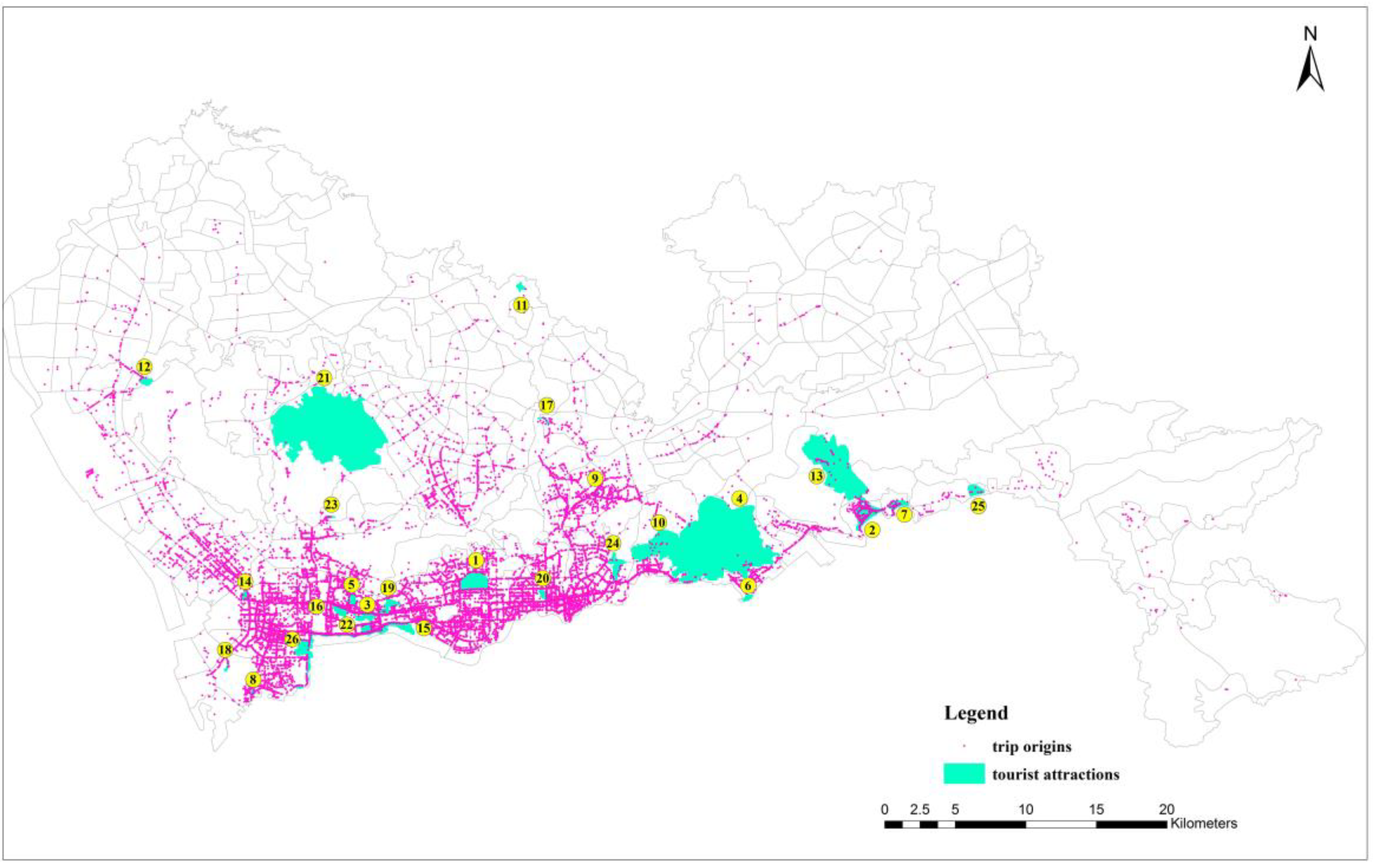
http://wtl.sz.gov.cn/, accessed on 26 June 2021). In the same year, taxi travel accounted for 10.5% of public transport travel in Shenzhen. To investigate the characteristics of tourism travel by taxi, we selected the top 26 attractions ranked by tourists on Ctrip.com (a popular Chinese travel booking and travel diary sharing website) and the taxi trips to these 26 attractions from May 1 to 3, 2015. These attractions are shown in Figure 1 and listed in Table 1. As can be seen on Figure 1, taxi trip origins are mainly distributed in three regions of Nanshan, Futian, and Luohu, where there are more tourist attractions.
The trajectory data were collected by 16,828 GNSS (Global Navigation Satellite System)-equipped taxis operating in Shenzhen, with an average sampling frequency of 30 s. In total, there are 69.16 million GNSS records. Each record includes the taxi’s identification, coordinates (i.e., latitude and longitude), instantaneous speed, time, and occupancy state (loading passengers or not). To explore the relationship between tourist trip origins and geographic contextual factors, this study also used POI (Point of Interest) data and road network data. The POI data were crawled from the open API of Gaode Maps (https://lbs.amap.com/api/webservice/guide/api/search, accessed on 26 June 2021), with over 1.7 million records as of the end of September 2018 [30], and each POI record includes attributes such as name, address, type, longitude, and latitude. The POI data are divided into 11 types: catering services (CS); corporate enterprise services (CES); shopping services (SS); transportation facilities (TF); finance and insurance services (FIS); science, education and culture services (SECS); residential housing (RH); living services (LS); sports and leisure services (SLS); health care services (HCS); and accommodation services (AS).

2.2. Methods

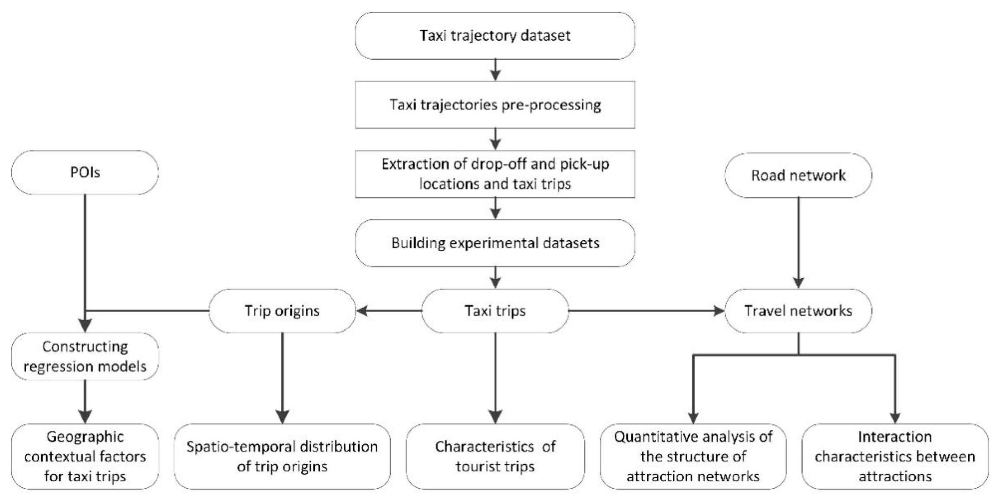
The spatial structure of urban tourist trips contains three components: trip origins, tourist attractions, and travel networks. To analyze the spatiotemporal characteristics of tourist trips from both supply and demand perspectives, we first processed the taxi trajectories to extract the tourist trips. Second, we analyzed the aggregation trends and spatial dependence of tourist trip origins and their correlations with geographic contextual factors by using KDE, Getis-Ord Gi*, and GWR. Third, we established tourist travel networks and analyzed their structure and characteristics using complex network metrics to explore the mechanism of the formation of the tourist network for each attraction. The methodology in this paper is divided into the following parts: building a tourist trip dataset, spatial aggregation of tourist trip origins and spatial dependence on geographic contextual factors, and quantitative analysis of the travel network structure for each attraction. All data analysis was conducted on a Dell Tower 7810 server with an Intel Xeon CPU, 32 GB of RAM. Taxi trajectory data were pre-processed using the Python. Tourist trip data was mapped and spatially analysed using ArcGIS.
The methodological framework is illustrated in Figure 2.
Step 1: Building tourist trip dataset.
The original collected taxi trajectories are disorganized, and tourist trips need to be extracted for subsequent tasks.
(1) Extraction of taxi trips.
We first identified and removed trajectory records with large latitude and longitude jumps and speed anomalies. Next, we used a map-matching algorithm called ST-Matching [31] to align all trajectory points (identified by ride status) between passenger pick-up and drop-off locations (identified by the occupancy states) with the road network.
(2) Selecting taxi trips for tourism.
The taxi trip data are divided into two types of trips: tourist trips and residential trips (i.e., trips for other activities of local residents). First, we sketched out the tourist drop-off areas of 26 tourist attractions to extract tourist trips. Considering the randomness of taxi drop-off locations and the influence of satellite positioning accuracy, we repeatedly compared and corrected the boundaries of the potential drop-off area of each attraction near the entrance with the help of Google satellite images and Baidu Street View (https://map.baidu.com/, accessed on 26 June 2021) to ensure the reliability of the extracted tourist trips. If the taxi drop-off location is in the potential drop-off area of a tourist attraction, this trip is considered to be a tourist trip. The final tourist trip dataset contained 37,878 records.
Step 2: Spatial aggregation of tourist trip origins and spatial dependence on geographic contextual factors.
The taxi travel network comprises trip origins, trip routes, and trip destinations. Of these, trip origins are commonly used for predicting trip generation rates and trip distribution in the field of trajectory-based urban travel studies, as well as for traffic impact, association relationship, and driver factors analysis. In this step, we focus on the aggregation trends of tourist trips by taxis, the spatial dependency characteristics, and the influence of geographical contextual factors.
(1) Aggregation trends and spatial dependencies of tourist trip origins.
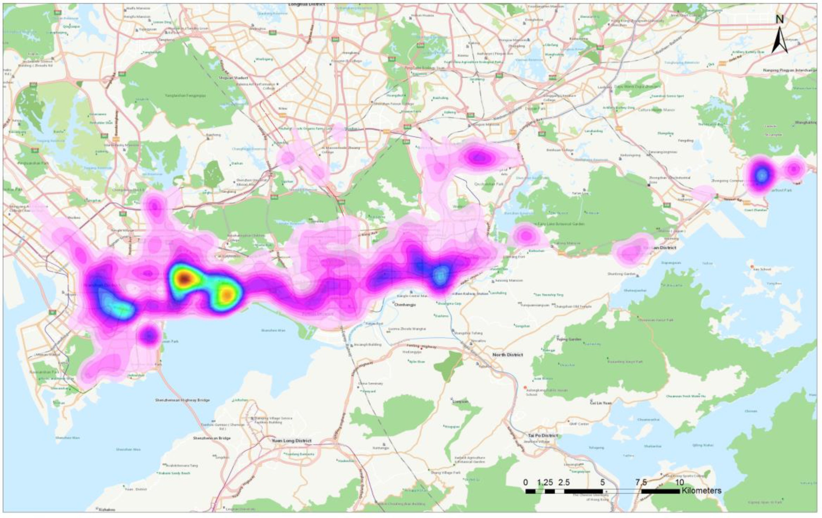
We used kernel density (KDE) (https://desktop.arcgis.com/en/arcmap/10.3/tools/spatial-analyst-toolbox/kernel-density.htm, accessed on 26 June 20211) [32] to estimate the aggregation trends of trip origins. KDE is a non-parameter calculation algorithm for surface density, which calculates the data aggregation status of the entire region based on the input dataset, to produce a continuous surface with density. A larger kernel density value indicates a stronger concentration—i.e., more tourists traveling from this location.
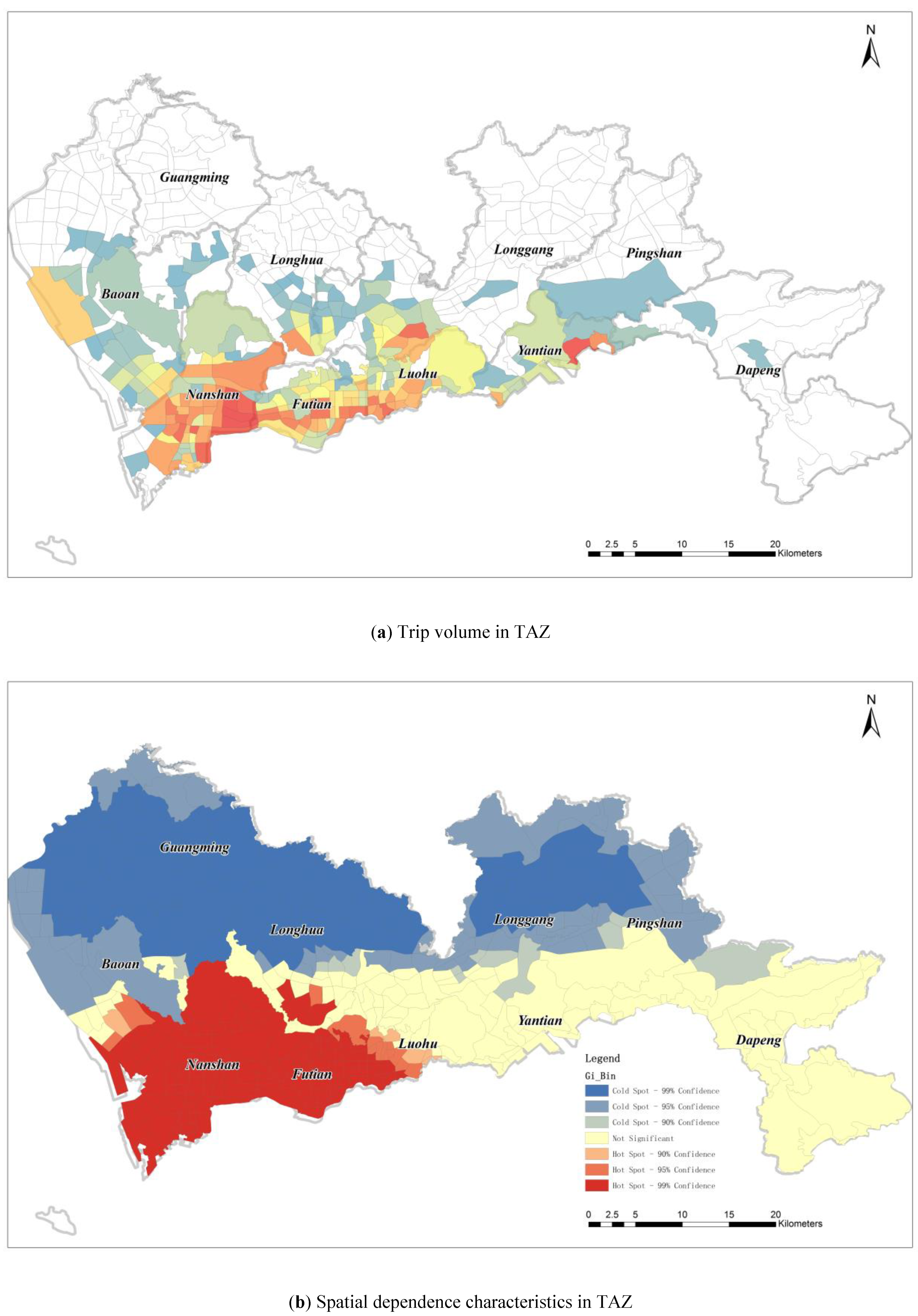
Next, we used the Getis-Ord Gi* (https://pro.arcgis.com/en/pro-app/latest/tool-reference/spatial-statistics/h-how-hot-spot-analysis-getis-ord-gi-spatial-stati.htm, accessed on 26 June 2021) [33] algorithm to explore the local spatial dependence of the tourist trip origins to determine the hot or cold regions for tourism travel. The Gi* statistic is the ratio of the sum of observations at locations around the target location to the sum of locations at all locations within a given distance range. It is used to identify whether there is a dependence between the target location and the surrounding locations in terms of high and low values. The Gi* statistic returns the z-score value for each element in the dataset. For positive z-scores, the higher the z-score, the tighter the spatial dependence for higher values. For negative z-scores, the lower the z-score, the tighter the spatial dependence for lower values. Thus, the Gi* statistic can identify significant hot spots (high-value spatial dependence) and cold spots (low-value spatial dependence).
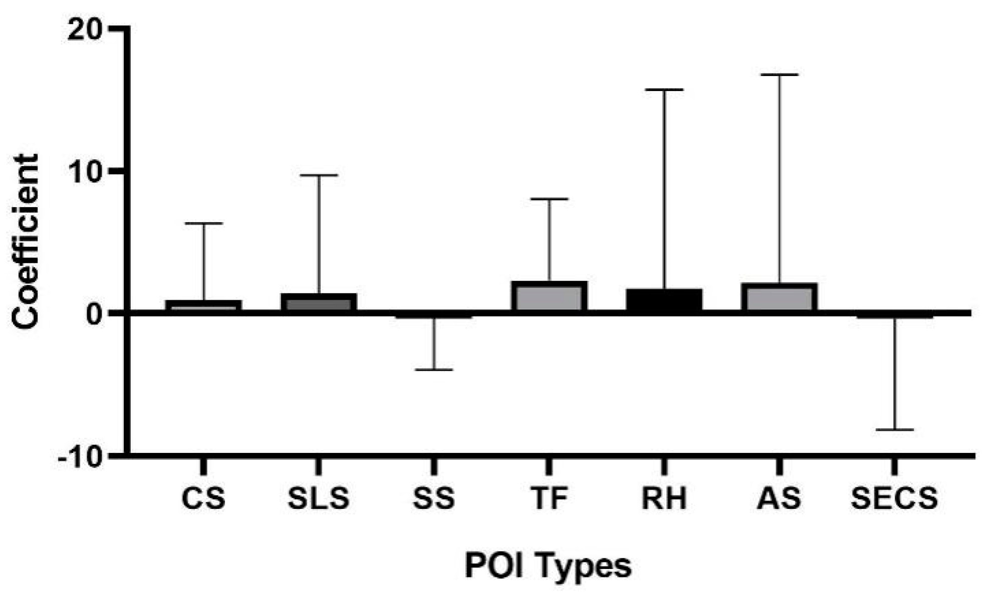
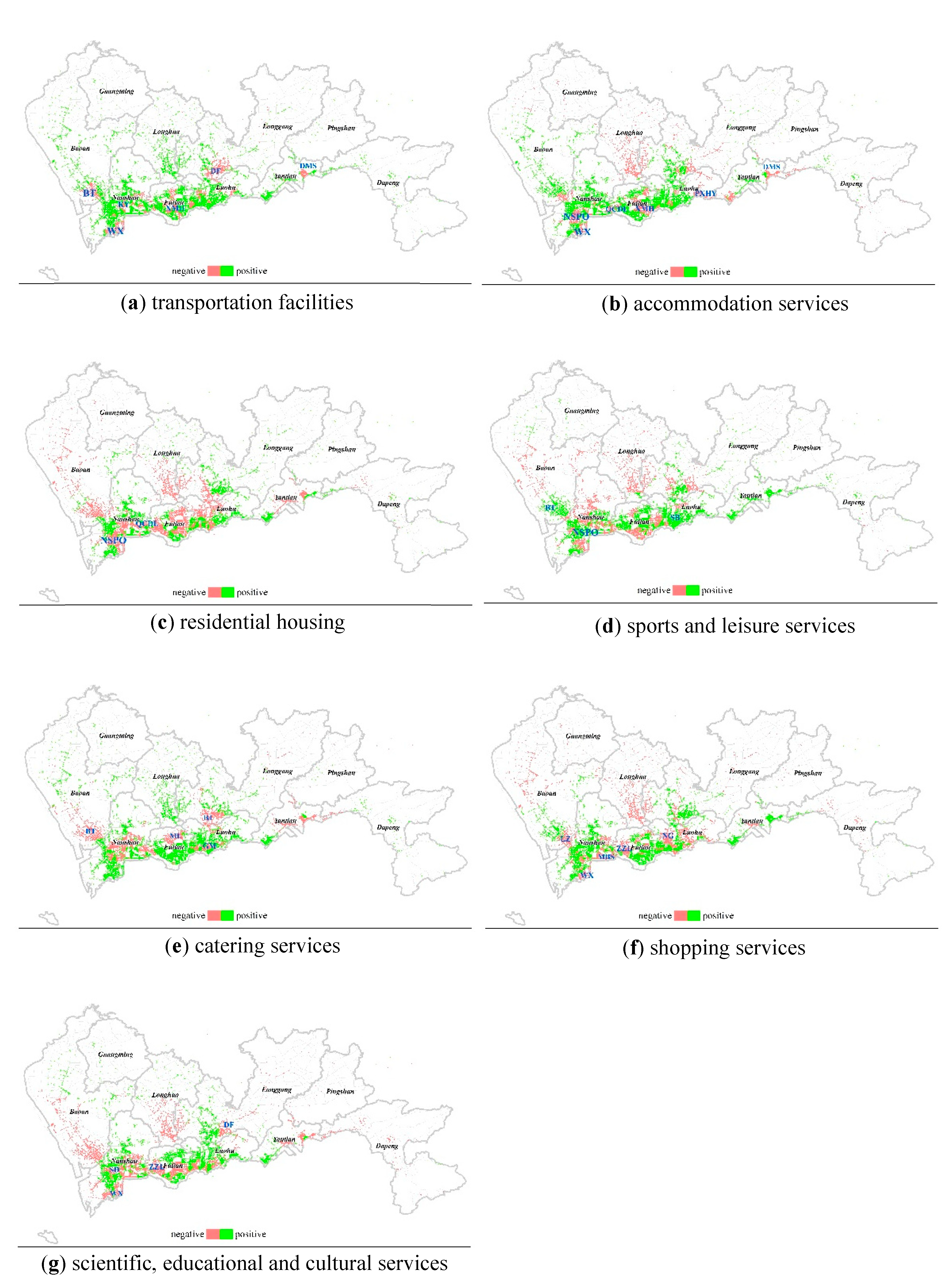
(2) Correlation between geographic contextual factors and trip origins.
To identify the factors correlated with trip origins, we created buffers with radii of 20, 50, 100, 200, and 300 m at each trip origin and counted the number of each type of POI within each buffer. We used the number of the 11 POI types as the optional explanatory variable and the kernel density value at the trip origin as the dependent variable to build a geographically weighted regression model, which was used to test the validity of the explanatory variables. Geographically weighted regression (GWR) (https://pro.arcgis.com/en/pro-app/latest/tool-reference/spatial-statistics/geographically-weighted-regression.htm, accessed on 26 June 2021) [34] introduced geographic location into the model parameters and used locally weighted least squares for parameter estimation. Therefore, the variables vary with spatial location and its model coefficients can better reveal the spatial non-homogeneity of geographic elements.
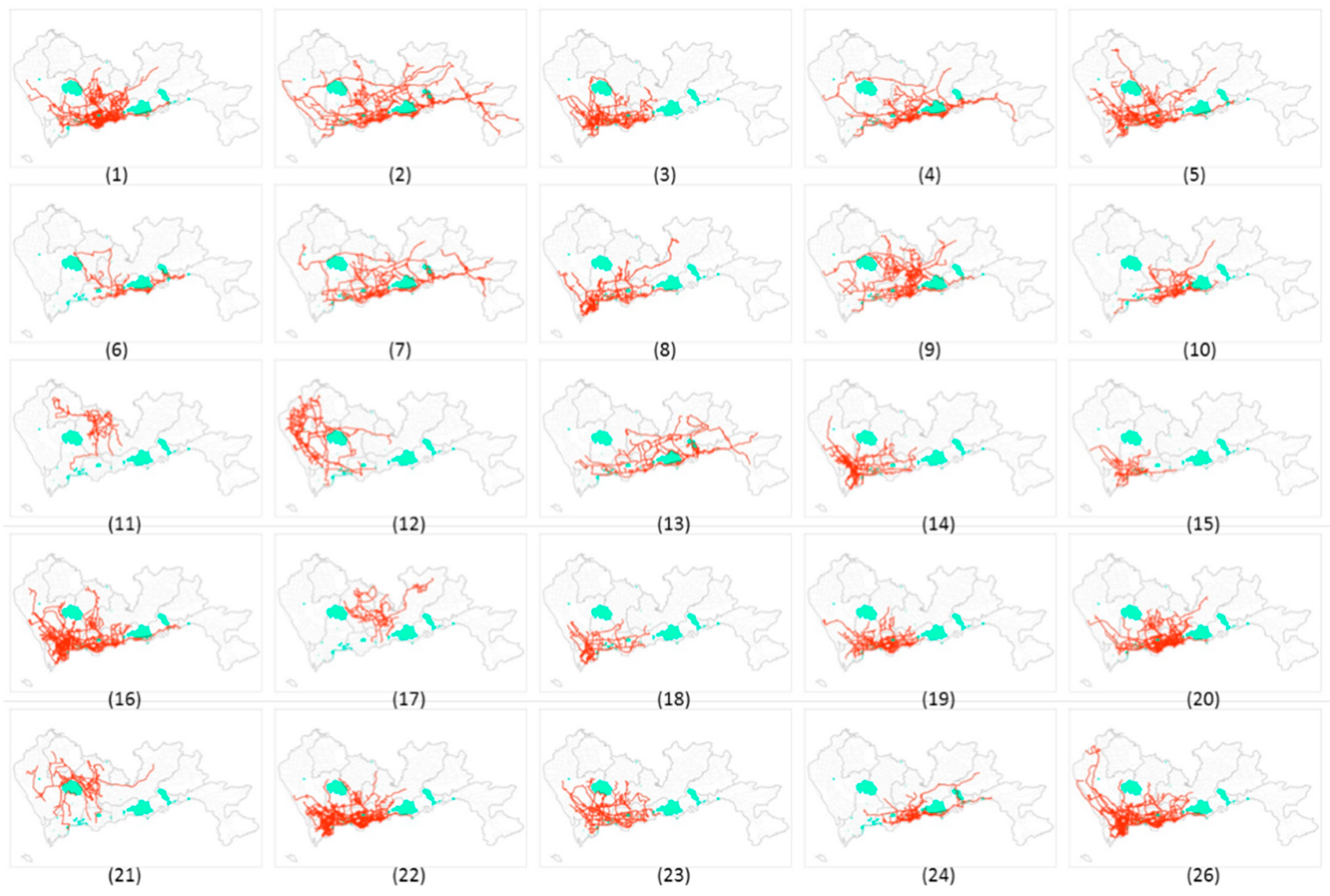
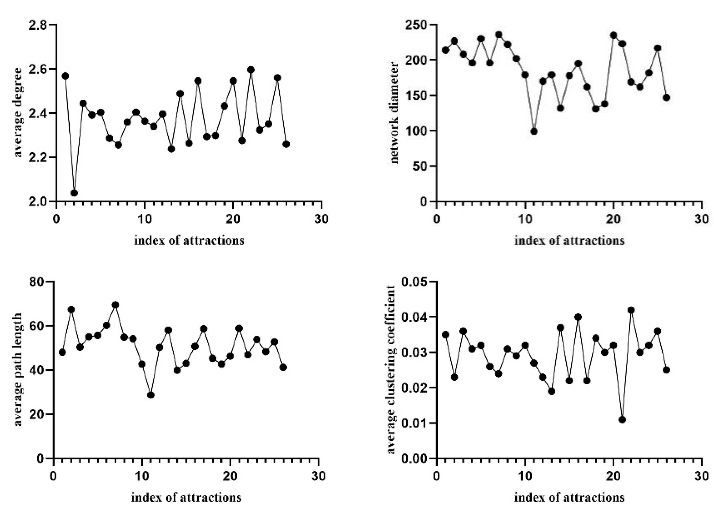
Step 3: Quantitative analysis of tourists’ travel networks.
Finally, 26 travel networks were created for each tourist attraction based on the tourist trip data. The nodes of a travel network comprise the trip origins, the road intersections through which travel routes pass and target tourist attractions. The edges of a travel network are composed of sections between road intersections. The resulting travel network integrates discrete trip origins and tourist attractions into a holistic system that can represent the spatial range of attractiveness and services of each attraction. To compare the structural differences in travel networks, complex network metrics such as average degree, network diameter, average path length, and average clustering coefficient were used. The specific details of each metric are not presented here and can be found in the relevant literature [35].

3. Results

3.1. Spatiotemporal Characteristics of Tourist Trips

To analyze the differences between the trip types, we counted the number of trips per hour. The horizontal axis in Figure 3 represents 72 time slots in three days. Figure 3a shows the volume of residential trips from May 1 to May 3, and Figure 3b shows the number of tourist trips to the 26 attractions. As shown in the figures, residential travel shows a cyclical pattern. The least number of trips is at 06:00. Subsequently, the travel volume gradually increases. The peak travel times are 11:00, 15:00, and 23:00. Unlike residential trips, there are two peak times for tourist trips—11:00 and 15:00—and the lowest tourism volume occurs at 05:00. Another difference between the two is that during ‘May Day’, daily residential trips show the same trend, with similar peak sizes; traffic to attractions, however, show a downward trend, with the lowest volume occurring on the last day of the holiday.
Figure 4a,b show the travel time and distance of tourist trips, respectively. In terms of travel time, short-distance trips of less than 15 min are larger, accounting for 67.89%, and trips of less than 45 min account for 95.48% of tourist travel traffic. This indicates that most travel activities during the holidays are mainly short-distance trips, and only a few people spend a long time engaged in travel activities. In terms of travel distance, trips within 8 km are larger, accounting for nearly 71.25%, and 94.86% of the trips occur within 23 km. Although the trends in Figure 4a,b are similar, there are minor differences, such as the existence of a plateau around 20 km, which shows a long tail and is not very smooth. We fitted the travel time and distance distributions, and after comparing the power law distribution, the gamma distribution, and the generalized extreme value distribution (GEV, as shown in Equation (1)) (https://www.mathworks.com/help/stats/generalized-extreme-value-distribution.html, accessed on 26 June 2021), we found that the GEV better reflects the climbing and falling trend of travel time and travel distance. After calculation, the GEV distribution function for travel time had parameters of k 0.3441, σ 2.0386, and μ 2.8441. The GEV distribution function for the travel distance had parameters of k 0.4342, σ 16.6224, and μ of 19.822.
f ( x ) = ( 1 σ ) exp ( ( 1 + k ( x μ ) σ ) 1 k ) ( 1 + k ( x μ ) σ ) 1 1 k
To characterize the travel volume on 491 traffic analysis zones (TAZs) during the ‘May Day’, we conducted a spatial dependency analysis of trip origins (as shown in Figure 5). Figure 5a shows that the TAZs with numerous trips are Baishizhou, Hongshuwan, Huaqiaochen, Dameisha, Haiyabaihuo, and Guomao. TAZs with a high volume of tourist trip origins can be divided into three types. The first type includes TAZs with popular attractions, such as OCT East, Dameisha Waterfront Park, and Xiaomeisha Waterfront Park. This type of TAZ is less popular, but most trips occur in taxis. The second type is transportation hubs, such as Luohu Port and Baoan Airport, where taxi trips to tourist attractions are more frequent. The third type is densely populated residential areas, such as Zhuzilin. However, there are also some areas where no taxi trips occur, such as Guangming District, northern Longgang, northern Pingshan, and the Dapeng District. Figure 5b shows the spatial dependence characteristics using the Getis-Ord Gi* optimization statistics tool. In Figure 5b, the red color indicates the spatial dependence of high values, and the blue color indicates the spatial dependence of low values. The results show that the TAZs with high trip volumes are concentrated in the south, including the Nanshan and Futian districts. The TAZs with low trip volumes are located in Guangming, Longgang, and parts of Bao’an, Longhua, and Pingshan.

3.2. Correlation between Tourist Trip Origins and Geographic Contextual Factors

To identify the aggregation trend at trip origins, we performed kernel density estimation with 30, 50, 100, 150, 200, 250, and 300 m as bandwidths. The experimental results indicate that the distribution pattern of the trip aggregation area on the density map is similar. Here, we take the density map at 100 m bandwidth as an example. Figure 6 indicates that the main travel aggregation area during ‘May Day’ includes four areas: Shenzhen Railway Station, the Damaisha scenic area, Happy Valley, and Hongrui Community.
For modeling the correlation between the spatial variation of tourist origins and the distribution of geographic environmental factors during the peak tourist season, a GWR model was developed using POI data and tourist trip origin data. First, we extracted the density values of each trip origin from seven kernel density maps—30, 50, 100, 150, 200, 250, and 300 m—and then established buffer zones with the corresponding size at each trip origin and extracted the number of each type of POI within buffer zones. At each scale, we chose the kernel density value at trip origin as the dependent variable and the number of 11 types of POI as the alternative explanatory variable. We examined and screened the independent variables under each of the seven scales using the OLS algorithm. The criteria for variable screening and modeling were (1) to ensure successful modeling, (2) to be able to explain tourist trip characteristics, (3) to satisfy significance tests, and (4) to avoid multicollinearity and spatial correlation. The final goodness-of-fit of the model was 0.9489 under a bandwidth and buffer of 100 m. R2-Adjusted, it was 0.948554. Seven categories of geographic environmental factors—CS, SLS, TF, RH, AS, SS, and SECS—were selected as the final explanatory variables in the GWR model.
The regression coefficients of the geographic environmental factors differed significantly, among which the mean values of five factors—CS, SLS, TF, RH, and AS—are positive for tourist travel, and those of the coefficients of SS and SECS are negative for tourist travel. The statistical results of the correlation coefficients of the POI for each type are shown in Figure 7. Among the factors that have a positive mean value of coefficients, the ranking is: TF, AS, RH, SLS, and CS; and the ranking of the means of negative coefficients is SS and SECS.
We visualized the regression coefficients spatially. Figure 8 shows that the POIs negatively correlate with tourist trips in red color and are positively correlated in green color. The main TAZs are labeled in Figure 8a–g. They include Wanxia Station (WX), Keyuan Station (KY), Xiangmihu Station (XMH), Dafen Station (DF), Baoti Station (BT), Dameisha (DMS), Nanshan Post Office (NSPO), Pengxinghuayuan (PXHY), Qiaocheng East Road (QCDL), Buji Station (BJ), Meilin Station (ML), Guomao Station (GM), Linzhi Station (LZ), Linzhi Station (LZ), Nigang Station (NG), Zhuzilin Station (ZZL), Mangrove Bay Station (MBS), and Shaibu Station (SB). The figures show that the regression coefficients are highly spatially heterogeneous. The correlations of different types of POIs with tourist trips vary considerably in each administrative district. For example, in the Baoan District, there is a positive correlation between transport facilities and accommodation services, and a negative correlation with residential housing. In Longhua District, there is a positive correlation between transport facilities and catering services, while accommodation services, residential facilities, and sports and leisure services are negatively correlated. Nanshan, Futian, and Luohu exhibit heterogeneity in the correlations between the various types of tourist facilities within them.

3.3. Structural Characteristics of Tourist Travel Networks

To explain the connections between the tourist attractions and how the tourism flow network is shaped, taxi trajectories associated with 26 attractions were selected from the taxi trip data to build travel networks of attractions. Figure 9 shows the travel networks for the 25 tourist attractions, and they clearly show the spatial coverage of the 25 attractions. Notably, Rose Coast has a smaller attraction network and is not plotted here. The figure shows that (1), (2), (4), (5), and (7) cover the widest range; they are: Lianhuashan Park, Dameisha Waterfront Park, Wutongshan Park, Happy Valley, and Xiaomeisha Waterfront Park. Figure 9(6), (10), (11), (14), (15), (17), (18), and (24) have the smallest spatial extent: Zhongyingjie, Xianhu Botanical Garden, Guanlan Printmaking Village, Holland Shenzhen Flower Town, Hongshulin Natural Conservation District, and Gankeng Hakka People Small Town. The remaining areas are the most densely covered: Jinxiu China Folk-Custom Village, Sea World, Fenghuangshan Forest Park, OCT East, Window of World, and International Garden & Flower Expo Park.
In addition, we divided the number of road sections of the travel network by the total number of road sections in Shenzhen to obtain the coverage of each tourist attraction. The statistical results of the coverage ratio for each attraction are shown in Figure 10. The four attractions with the greatest coverage are (1), (16), (22), and (26)—Lianhuashan Park, Window of World, Happy Coast, and Talent Park. The ones with the least coverage are (11), (17), and (25)—Guanlan Printmaking Village, Gankeng Hakka People Small Town, and Rose Coast.
Furthermore, the number of tourist trips by taxi for each attraction is summarized in the stacked bars shown in Figure 11. The blue, light green, and dark green bars show the number of tourist trips for each attraction on May 1st, 2nd, and 3rd respectively. If the number of tourists increases daily, only the last day’s number of tourists can be seen. If the number of tourists decreases, the tourist volume for three days can be seen. In the remaining the cases, only two days’ tourist volumes can be seen. The figure shows that the tourist volume at attractions (1), (4), (5), (8), (9), (20), and (24) decreases daily, where (1) and (24) have less decreasing tourist volume for the first two days. Attractions that reached their peak on the second day are (2), (3), (7), (14), (15), (16), (18), (19), (22), (23), and (26).
We calculated complex network metrics for 26 attractions using four metrics per attraction (as shown in Table 1). The results are illustrated in Figure 12. For the average degrees, the largest value is (22) Happy Coast, and the smallest value is (2) Dameisha Waterfront Park. The largest network diameter is (7) Xiaomeisha Waterfront Park, and the smallest value is (11) Guanlan Printmaking Village. For the average path length, the largest value is (7) Xiaomeisha WaterFront Park, and the smallest value is (11) Guanlan Printmaking Village. For the average clustering coefficients, the largest value is (22) Happy Coast, and the smallest value is (21) Yangtaishan Forest Park.
We created a spatial interaction intensity map between attractions (shown in Figure 13) using the number of tourist trips between different attractions. In Figure 13, the nodes indicate the 26 tourist attractions, and the edges indicate the flow connection between the attractions. We used the natural breakpoint method to divide the number of tourist trips into three classes. The red edges have the highest number of trips, the blue edges have the second highest, and the lowest is the grey edges. Notably, the internal attractions in the east and west are closely linked, while the surrounding attractions are less connected. The Window of World, Jinxiu China Folk-Custom Village, Happy Coast, and Happy Valley have the highest trip volumes, forming a tight cluster. The main flow of tourists between the east and west attractions lies between Dameisha and Window of World. The Qingqing World, Holland Shenzhen Flower Town, Safari Park, Dafen Village, and Zhongyingjie are located at the boundary of the network structure, and the scenic nodes are sparsely connected to other nodes. Furthermore, the abovementioned also indicates that tourist flows during the holiday period are mainly concentrated in areas with better tourism development, dense, and rich resources, and high accessibility.

4. Discussion

(1) Analysis of tourism travel models.
For the distribution model, there are various models to describe the distribution patterns of travel distance and travel time in trajectory data, such as power law distribution, exponential distribution, exponentially truncated power law distribution, lognormal distribution, and gamma distribution. Brockmann [36] observed that human travel distances show a power law distribution. Yan [37] argued that the mode of transportation affects the aggregated travel patterns, and the displacement from a single mode traffic should follow an exponential distribution rather than a power law. Liang [38] argued that the displacement of taxi passenger trips follows an exponential decay. Zhang explored urban mobility in Harbin, China, and found that travel distances follow a log-normal distribution [39]. Veloso found that the gamma distribution can describe the travel distance of taxis [
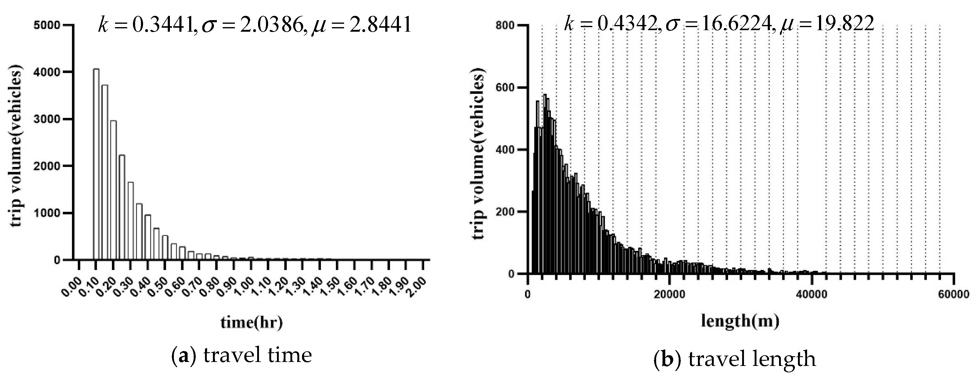
40]. From the above studies, it can be seen that the travel time and distance patterns contained in the trajectory data are difficult to represent using a uniform model in different data sets and study areas. In this study, through the modeling and comparative analysis of travel distances, we found that the GEV model better represents the characteristics of tourist trips on ‘May Day’. It can describe the climbing and falling characteristics in trips. In line with the pattern derived from the other data, all data fall into the long-tail distribution, which represents a decreasing volume of traffic over long distances. However, the GEV fits the data better in describing the climbing characteristics. One of the possible reasons for this is that the combination of the layout characteristics of tourism resource and the weather factors lead to the need for more comfortable transportation when visiting the close attractions. This phenomenon could describe the preference of tourists for taxi travel, which would help to plan an efficient and effective transport system that facilitates the turnover of tourists between multiple attractions. Moreover, this phenomenon is expected to guide them in making informed decisions about transportation services when visiting multiple attractions.
For travel mobility models, most of the previous literature has given flow patterns between destinations [41]. In contrast, few studies have been devoted to modelling intra-destination flows. It is therefore important to clarify the patterns of intra-destination flows [42], particularly the characteristics of city-scale tourism flows. In many countries, taxis are the preferred mode of travel for many trips, especially for individuals conducting business and tourism. Existing studies of travel behavior using trajectory data focus on the transportation characteristics of commuters in general. In this study, we analyzed the structural characteristics of taxi travel networks between intra-city attractions. McKercher and Lew [43] gave four mobility patterns for tourists, such as single destination with or without side trips, transit leg and circle tour, circle tour with or without multiple access, and hub-and-spoke style. These patterns can be used to guide tourism product development. However, it is difficult to adapt to the needs of transportation organization and synergistic development planning among multiple attractions. We used taxi OD data and tourist volume to establish a flow network between multiple attractions. The results reported in this study shows that taxi trip data can reveal the spatial use behavior of tourism resources, which can be used to guide tourism product development, and tourism route organization and planning.
For the modeling of impact factors, a lot of meaningful work has been done. Urban taxi travel is closely related to geographic location, particularly sociodemographic distribution and built environment characteristics [1]. Compared to previous studies, this study focuses on the impact of the built environment. Considering the difficulty of obtaining taxi trajectory data and the demographic characteristics of tourists at the same time, we built a geographically weighted regression model with trip density as the dependent variable and POIs within the buffer as the explanatory variable to help explain the spatial imbalance of tourist trips. Since it is difficult to build the range of environmental factors influencing travel, we conducted a buffer zone analysis at seven different scales to build models that may accommodate more explanatory variables. Through experiments, we found that the modellable variables that can explain the characteristics of trip occurrence are different. At 100 m, the associated influence of various types of POI is more effectively expressed.
(2) Implications for tourism transportation planning.
This study analyzed the characteristics of urban tourist trips from a spatiotemporal and network perspective. The results show that the morphological structure of cities and the uneven distribution of tourism resources are one of the main reasons for the hot and cold distribution of tourist trips. In such a scenario, a single mode of transport affects the willingness and impression of urban tourism travel. Moreover, as a fast means of transport, the need for drivers to make a profit affects the spatial distribution of the passenger-finding process, as they prefer to go to places where there is a high population density. This also generates competitive pressure to travel. For urban tourism resources to be favoured by the public, the development of time-saving, long-distance transportation modes is a necessary part of a sustainable urban tourism system. Taking Shenzhen as an example, the data collection year for this study was 2015, when there were five metro lines and a lack of metro lines in the northern and eastern parts of the city. When taxis are not adequately distributed, the public has to rely on buses, which may lead to increased travel time and reduced willingness to travel. The Shenzhen government is also working to improve transport conditions, although the main goal is to serve the needs of daily commuting and mobility, which invariably also benefits the city’s tourism industry. As of 2020, Shenzhen has 11 metro lines, and travel conditions in the east and north have been significantly improved. Moreover, since 2016, Shenzhen has developed shared cars that can be hailed via smartphones and picked up at the departure point on time. These modes of transportation facilitate the tourism travel from long distances and bridge the imbalance in the spatial distribution of taxicabs carrying tourists. Overall, taxis are one of the most important parts of urban tourism transport systems. However, to achieve sustainable urban tourism, opening long-distance metros and increasing car sharing will help to satisfy tourism travel in suburban areas and improve the equity of urban tourism, the image of urban tourism and tourist satisfaction.
(3) Limitations.
There are various modes of transport that can be used for urban tourism, such as metros, buses, and taxis. Recently, car sharing has gradually emerged as a new transport mode for the public. This study focuses only on taxi travel during a single time period, ‘May Day’, which has limitations in terms of the comprehensiveness of the transport modes. However, the related data analysis methods are applicable to other transport modes, and the results are reliable when compared to traditional manual tourist surveys, especially for transport modes such as taxis where on-site survey data is difficult to collect. Another limitation is the extraction methods for tourist trips. Given the random nature of taxi drop-off locations, it is difficult to define a precise area at the entrance of a tourist attraction to assist in extracting reliable trips. However, we tried to ensure the quality of the data and the accuracy of the drop-off areas, such as, by setting different drop-off areas for different attraction entrances and road layouts, and by combining Baidu Street View and Google satellite images to correct the drop-off areas to take into account the congestion of tourist traffic in ‘May Day’.

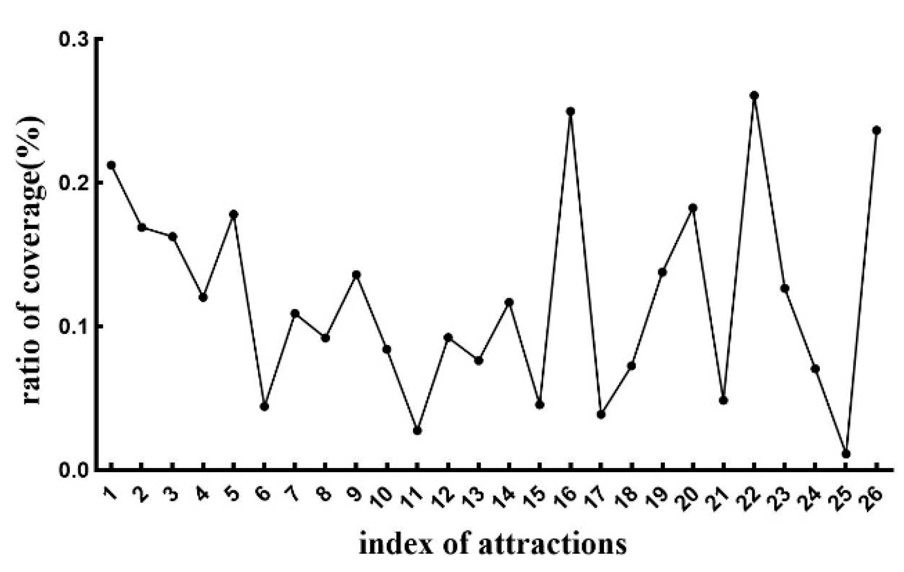
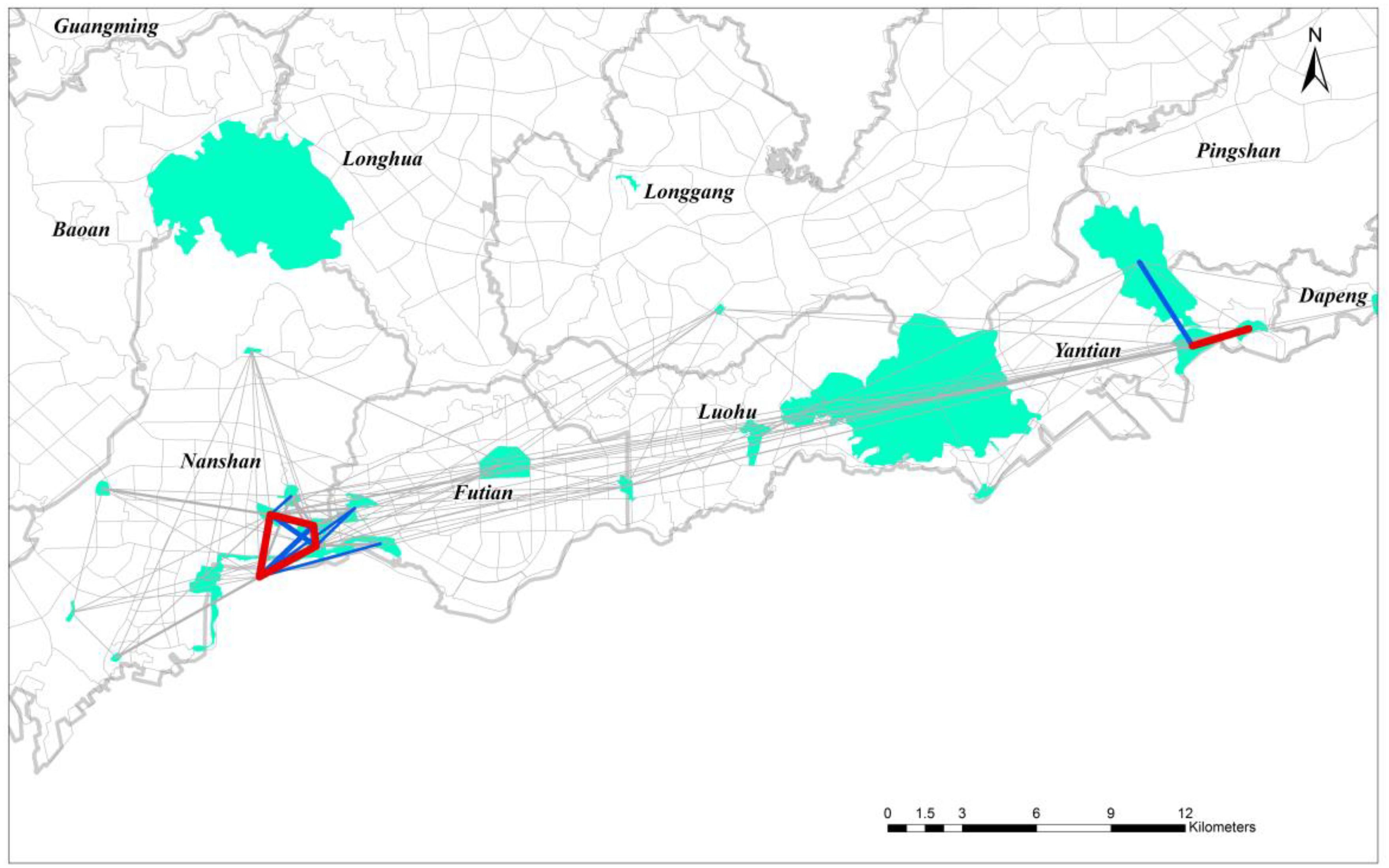
5. Conclusions and Future Work

In this study, we investigated the spatial distribution characteristics of tourist trip origins and their correlation with geographical contextual factors, as well as the structural characteristics of tourist travel networks. First, we used the KDE algorithm to analyze the spatial aggregation characteristics of tourist trip origins. The results show that tourist trips are concentrated in areas with a high distribution of tourist attractions and urban entry/exit ports. Second, we examined the spatial dependence of tourist trips using Getis-Ord Gi* and found that urban spatial structure, morphological characteristics, and the distribution of tourist resources can have an impact on tourist taxi trips. Third, we explored the correlations between the tourist trip origins and urban geographic contextual factors using the GWR model. The results revealed significant differences in the correlations between tourist trips and the factors. Finally, we constructed travel networks and quantified and compared them using complex network metrics. Other interesting insights were found that are either consistent or inconsistent with some preconceived ideas and related research. First, the trend between the coverage of the tourism network and the volume of tourist trips is similar. Furthermore, for attractions with high coverage, the peak in tourist volumes occurs on the second day of the tourism period. Attractions in the middle of the coverage rankings show a downward trend in tourist volumes. Second, the spatial interaction intensity between urban tourist attractions has two structural characteristics: grouping and hierarchy. However, the groups are not evenly distributed spatially. This is one of the reasons why there is a big difference between the hot and cold tourist trips from the north and south of Shenzhen.
Compared with other public transport data, taxi GNSS records have higher accuracy for location and time stamping, which can reveal people’s movement patterns with reliability. Here, we have only analyzed the tourist characteristics in ‘May Day’, and in the future, we aim to obtain data for the same period over several years and carry out a comparative analysis covering other tourist seasons in China, such as the National Day. Moreover, we will focus on the environmental semantic features of traffic around tourist attractions to assist in tourism product development and tourist moderation.

Author Contributions

Conceptualization, methodology, writing—review and editing, Bing He and Kang Liu; resources, data curation, Kang Liu; data pre-processing Guohua Wu and Jiyao Yin; visualization, Zhe Xue and Jiajun Liu; Diping Yuan revised the manuscript. All authors have read and agreed to the published version of the manuscript.

Funding

This research was supported by the National Natural Science Foundation of China (No. 41901391, 41701167), the Shenzhen Fundamental Research Program (No. JCYJ20190812171419161, JCYJ20190807163001783), and a grant from State Key Laboratory of Resources and Environmental Information System.

Institutional Review Board Statement

Not applicable.

Informed Consent Statement

Not applicable.

Data Availability Statement

As the data also form part of an ongoing study, the raw data needed to reproduce these findings cannot be shared at this time.

Conflicts of Interest

The authors declare no conflict of interest.

References

  1. Qian, X.W.; Ukkusuri, S.V. Spatial variation of the urban taxi ridership using GPS data. Appl. Geogr. 2015, 59, 31–42. [Google Scholar] [CrossRef]
  2. Nutsugbodo, Y.R.; Amenumey, E.K.; Mensah, C.A. Public transport mode preferences of international tourists in Ghana: Implications for transport planning. Travel Behav. Soc. 2008, 11, 1–8. [Google Scholar] [CrossRef]
  3. Cheng, H.M.; Li, S.Y.; Ning, Y.Z.; Chen, X.; Pan, R.; Zhang, Z.Y. Analysis on utilization of Beijing local roads using taxi GPS data. Phys. A 2020, 545, 1–9. [Google Scholar] [CrossRef]
  4. Lew, A.; McKercher, B. Modelling tourist movements: A local destination analysis. Ann. Tour. Res. 2006, 33, 403–423. [Google Scholar] [CrossRef]
  5. Shih, H.Y. Network characteristics of drive tourism destinations: An application of network analysis in tourism. Tour. Manag. 2006, 27, 1029–1039. [Google Scholar] [CrossRef]
  6. Park, S.W.; Xu, Y.; Jiang, L.; Chen, Z.L.; Huang, S.Y. Spatial structures of tourism destinations: A trajectory data mining approach leveraging mobile big data. Ann. Tour. Res. 2020, 84, 1–17. [Google Scholar] [CrossRef]
  7. Zheng, W.M.; Zhou, R.; Zhang, Z.M.; Zhong, Y.H.; Wang, S.R.; Zhao, W.; Ji, H.P. Understanding the tourist mobility using GPS: How similar are the tourists. Tour. Manag. 2018, 71, 54–66. [Google Scholar] [CrossRef]
  8. Zhang, K.; Chen, Y.; Li, C.L. Discovering the tourists’ behaviors and perceptions in a tourism destination by analyzing photos’ visual content with a computer deep learning model: The case of Beijing. Tour. Manag. 2019, 75, 595–608. [Google Scholar] [CrossRef]
  9. Wang, F.; Peng, X.; Qin, Y.L.; Wang, C.S. What can the news tell us about the environmental performance of tourist areas? A text mining approach to China’s national 5A tourist areas. Sustain. Cities Soc. 2020, 52, 1–12. [Google Scholar] [CrossRef]
  10. Hasnat, M.M.; Hasan, S. Identifying tourists and analyzing spatial patterns of their destinations from location–based social media data. Transp. Res. Part C Emerg. Technol. 2018, 96, 38–54. [Google Scholar] [CrossRef]
  11. Liu, X.; Gong, L.; Gong, Y.X.; Liu, Y. Revealing travel patterns and city structure with taxi trip data. J. Transp. Geogr. 2015, 43, 78–90. [Google Scholar] [CrossRef] [Green Version]
  12. Wang, Y.J.; Deng, Y.; Ren, F.; Zhu, R.X.; Wang, P.; Du, T.; Du, Q.Y. Spatial structure, intra–urban commuting patterns and travel mode choice: Analyses of relationships in the Kumasi Metropolis, Ghana. Cities 2020, 96, 1–20. [Google Scholar]
  13. Zhou, Y.; Fang, Z.X.; Thill, J.C.; Li, Q.Q.; Li, Y.G. Functionally critical locations in an urban transportation network: Identification and space–time analysis using taxi trajectories. Comput. Environ. Urban Syst. 2015, 52, 34–47. [Google Scholar] [CrossRef]
  14. Wang, T.Y.; Yue, W.Z.; Ye, X.Y.; Liu, Y.; Liu, D.B. Re–evaluating polycentric urban structure: A functional linkage perspective. Cities 2020, 101, 1–11. [Google Scholar] [CrossRef]
  15. Liu, Y.; Wang, F.H.; Xiao, Y.; Gao, S. Urban land uses and traffic ‘source–sink areas’: Evidence from GPS–enabled taxi data in Shanghai. Landsc. Urban Plan. 2012, 106, 73–87. [Google Scholar] [CrossRef]
  16. Yang, Y.; He, Z.; Song, Z.Y.; Fu, X.; Wang, J.W. Investigation on structural and spatial characteristics of taxi trip trajectory network in Xi’an, China. Physica A 2018, 506, 755–766. [Google Scholar] [CrossRef]
  17. Zhu, D.; Wang, N.H.; Wu, L.; Liu, Y. Street as a big geo–data assembly and analysis unit in urban studies: A case study using Beijing taxi data. Appl. Geogr. 2017, 86, 152–164. [Google Scholar] [CrossRef]
  18. Cai, H.; Zhan, X.W.; Zhu, J.; Jia, X.P.; Chiu, A.S.F.; Xu, M. Understanding taxi travel patterns. Physica A 2016, 457, 590–597. [Google Scholar] [CrossRef] [Green Version]
  19. Cui, J.X.; Liu, F.; Janssens, D.; An, S.; Wets, G.; Cools, M. Detecting urban road network accessibility problems using taxi GPS data. J. Transp. Geogr. 2016, 51, 147–157. [Google Scholar] [CrossRef]
  20. Kan, Z.H.; Tang, L.L.; Kwan, M.B.; Ren, C.; Liu, D.; Li, Q.Q. Traffic congestion analysis at the turn level using Taxis’ GPS trajectory data. Comput. Environ. Urban Syst. 2019, 74, 229–243. [Google Scholar] [CrossRef]
  21. Duan, Z.; Zhang, K.; Chen, Z.; Liu, Z.Y.; Tang, L.; Yang, Y.; Ni, Y.Y. Prediction of city–scale dynamic taxi origin–destination flows using a hybrid deep neural network combined with travel time. IEEE Access 2019, 99, 127816–127832. [Google Scholar] [CrossRef]
  22. Tulic, M.; Bauer, D.; Scherrer, W. Link and Route Travel Time Prediction Including the Corresponding Reliability in an Urban Network Based on Taxi Floating Car Data. Transp. Res. Rec. 2014, 2442, 140–149. [Google Scholar] [CrossRef]
  23. Yu, X.L.; Gao, S.; Hu, X.B.; Park, H. A Markov decision process approach to vacant taxi routing with e–hailing. Transp. Res. Part B Methodol. 2019, 121, 114–134. [Google Scholar] [CrossRef]
  24. Pan, G.; Qi, G.; Wu, Z.; Zhang, D.; Li, S. Land–use classification using taxi GPS traces. IEEE Trans. Intell. Transp. Syst. 2013, 14, 113–123. [Google Scholar] [CrossRef]
  25. Chen, E.; Ye, Z.R.; Wang, C.; Zhang, W.B. Discovering the spatio–temporal impacts of built environment on metro ridership using smart card data. Cities 2019, 95, 1–14. [Google Scholar] [CrossRef]
  26. Pan, Y.J.; Chen, S.Y.; Niu, S.F.; Ma, Y.F.; Tang, K. Investigating the impacts of built environment on traffic states incorporating spatial heterogeneity. J. Transp. Geogr. 2020, 83, 1–14. [Google Scholar] [CrossRef]
  27. Pearce, D.G. Toward an integrative conceptual framework of destinations. J. Travel Res. 2014, 53, 141–153. [Google Scholar] [CrossRef]
  28. Burns, P.M.; Novelli, M.M. Tourism and Mobilities: Local–Global Connections; CABI: Wallingford, UK; Cambridge, MA, USA, 2008. [Google Scholar]
  29. Baggio, R.; Scott, N.; Cooper, C. Network science–A review focused on tourism. Ann. Tour. Res. 2010, 37, 802–827. [Google Scholar] [CrossRef]
  30. Liu, K.; Yin, L.; Lu, F.; Mou, N.X. Visualizing and exploring POI configurations of urban regions on POI–type semantic space. Cities 2020, 99, 102610. [Google Scholar] [CrossRef]
  31. Lou, Y.; Zhang, C.Y.; Zheng, Y.; Xie, X.; Wang, W.; Huang, Y. Map–matching for low–sampling–rate GPS trajectories. In Proceedings of the 17th ACM SIGSPATIAL International Symposium on Advances in Geographic Information Systems, Seattle, WA, USA, 4–6 November 2009; pp. 352–361. [Google Scholar]
  32. Silverman, B.W. Density Estimation for Statistics and Data Analysis; Chapman and Hall: New York, NY, USA, 1986. [Google Scholar]
  33. Songchitruksa, P.; Zeng, X. Getis–Ord Spatial Statistics to Identify Hot Spots by Using Incident Management Data. Transp. Res. Rec. 2010, 2165, 42–51. [Google Scholar] [CrossRef]
  34. Fotheringham, A.S.; Zhan, F.B. A Comparison of three exploratory methods for cluster detection in spatial point patterns. Geogr. Anal. 1996, 28, 200–218. [Google Scholar] [CrossRef]
  35. Newman, M.E.J. The structure and function of complex network. SIAM Rev. 2003, 45, 167–256. [Google Scholar] [CrossRef] [Green Version]
  36. Brockmann, D.; Hufnagel, L.; Geisel, T. The scaling laws of human travel. Nature 2006, 439, 462–465. [Google Scholar] [CrossRef] [PubMed]
  37. Yan, X.Y.; Han, X.P.; Wang, H.B.; Zhou, T. Diversity of individual mobility patterns and emergence of aggregated scaling laws. Sci. Rep. 2013, 3, 2678. [Google Scholar] [CrossRef]
  38. Liang, X.; Zheng, X.; Lv, W.; Zhu, T.; Xu, K. The scaling of human mobility by taxis is exponential. Physica A Stat. Mech. Appl. 2012, 391, 2135–2144. [Google Scholar] [CrossRef] [Green Version]
  39. Zhang, S.; Tang, J.; Wang, H.; Wang, Y.; An, S. Revealing intra–urban travel patterns and service ranges from taxi trajectories. J. Transp. Geogr. 2017, 61, 72–86. [Google Scholar] [CrossRef]
  40. Veloso, M.; Phithakkitnukoon, S.; Bento, C.; Fonseca, N.; Olivier, P. Exploratory study of urban flow using taxi traces. In Proceedings of the First Workshop on Pervasive Urban Applications (PURBA) in Conjunction with Pervasive Computing, San Francisco, CA, USA, 10 October 2011. [Google Scholar]
  41. McKercher, B.; Lau, G. Movement patterns of tourists within a destination. Tour. Manag. 2008, 10, 355–374. [Google Scholar] [CrossRef]
  42. Masiero, L.; Zoltan, J. Tourists intra–destination visits and transport mode: A bivariate probit model. Ann. Tour. Res. 2013, 43, 529–546. [Google Scholar] [CrossRef]
  43. McKercher, B.; Lew, A. Tourist Flows and the Spatial Distribution of Tourists; A companion of tourism; Lew, A., Hall, C.M., Williams, A., Eds.; Blackwell: Oxford, UK, 2004; pp. 36–43. [Google Scholar]
Figure 1. The spatial distribution of tourist attractions and trip origins in Shenzhen, China.
Ijgi 10 00445 g001
Figure 2. Methodological framework.
Ijgi 10 00445 g002
Figure 3. (a,b) Hourly traffic volume of residential trips and tourist trips.
Ijgi 10 00445 g003
Figure 4. (a,b) Statistics on travel time and length of tourist trips.
Ijgi 10 00445 g004
Figure 5. (a,b) Spatial distribution characteristics of trip origins at TAZ scale.
Ijgi 10 00445 g005
Figure 6. Density distribution of travel origins.
Ijgi 10 00445 g006
Figure 7. Correlation coefficients with POIs.
Ijgi 10 00445 g007
Figure 8. (ag) Maps of regression coefficients.
Ijgi 10 00445 g008
Figure 9. Travel networks for tourist attractions.
Ijgi 10 00445 g009
Figure 10. Coverage of the travel networks.
Ijgi 10 00445 g010
Figure 11. Tourist flow distribution for attractions in three days.
Ijgi 10 00445 g011
Figure 12. Complex network metrics for the travel networks of each attraction.
Ijgi 10 00445 g012
Figure 13. Spatial interaction intensity of attractions.
Ijgi 10 00445 g013
Table 1. List of tourist attractions in Shenzhen.
IndexNameIndexNameIndexName
1Lianhuashan Park10Xianhu Botanical Garden19International Garden & Flower Expo Park
2Dameisha WaterFront Park11Guanlan Printmaking Village20Lychee Park
3Jinxiu China Folk-Custom Village12Fenghuangshan Forest Park21Yangtaishan Forest Park
4Wutongshan Park13OCT East22Happy Coast
5Happy Valley14Holland Shenzhen Flower Town23Safari Park
6Zhongyingjie15Hongshulin Natural Conservation District24Donghu Park
7Xiaomeisha WaterFront Park16Window of World25Rose Coast
8Sea World17Gankeng Hakka People Small Town26Talents Park
9Dafen Village18Qingqing World
Publisher’s Note: MDPI stays neutral with regard to jurisdictional claims in published maps and institutional affiliations.

