
Assessing the Urban Eco-Environmental Quality by the Remote-Sensing Ecological Index: Application to Tianjin, North China


Abstract
:1. Introduction
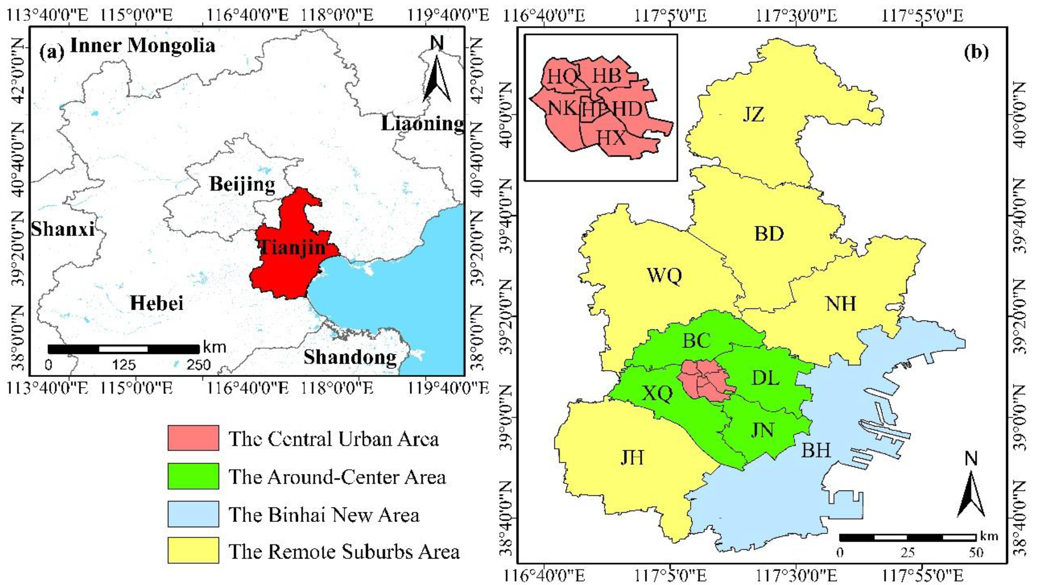
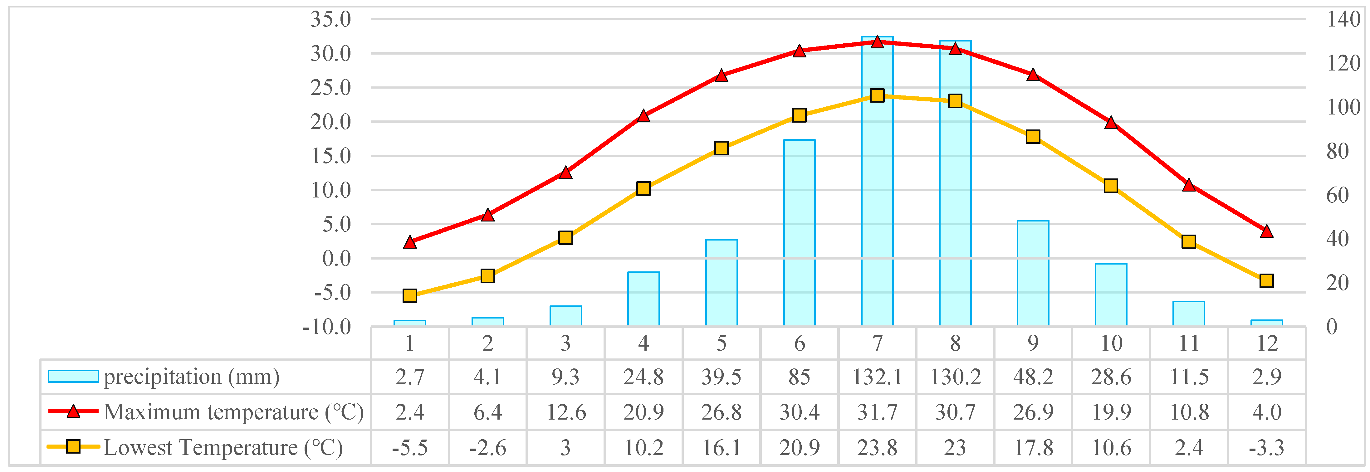
2. Study Area
3. Data and Methods
3.1. Remote-Sensing Data
3.2. Remote-Sensing Ecological Index (RSEI) Indicators
3.2.1. Greenness—Normalized Difference Vegetation Index (NDVI)
3.2.2. Moisture—Wetness (Wet Component)
3.2.3. Dryness—Normalized Difference Building-Soil Index (NDBSI)
3.2.4. Heat—Land Surface Temperature (LST)
3.3. RSEI Model
3.3.1. Normalization of the Measures
3.3.2. Water Masking
3.3.3. Integration of the Measures
4. Results and Discussion
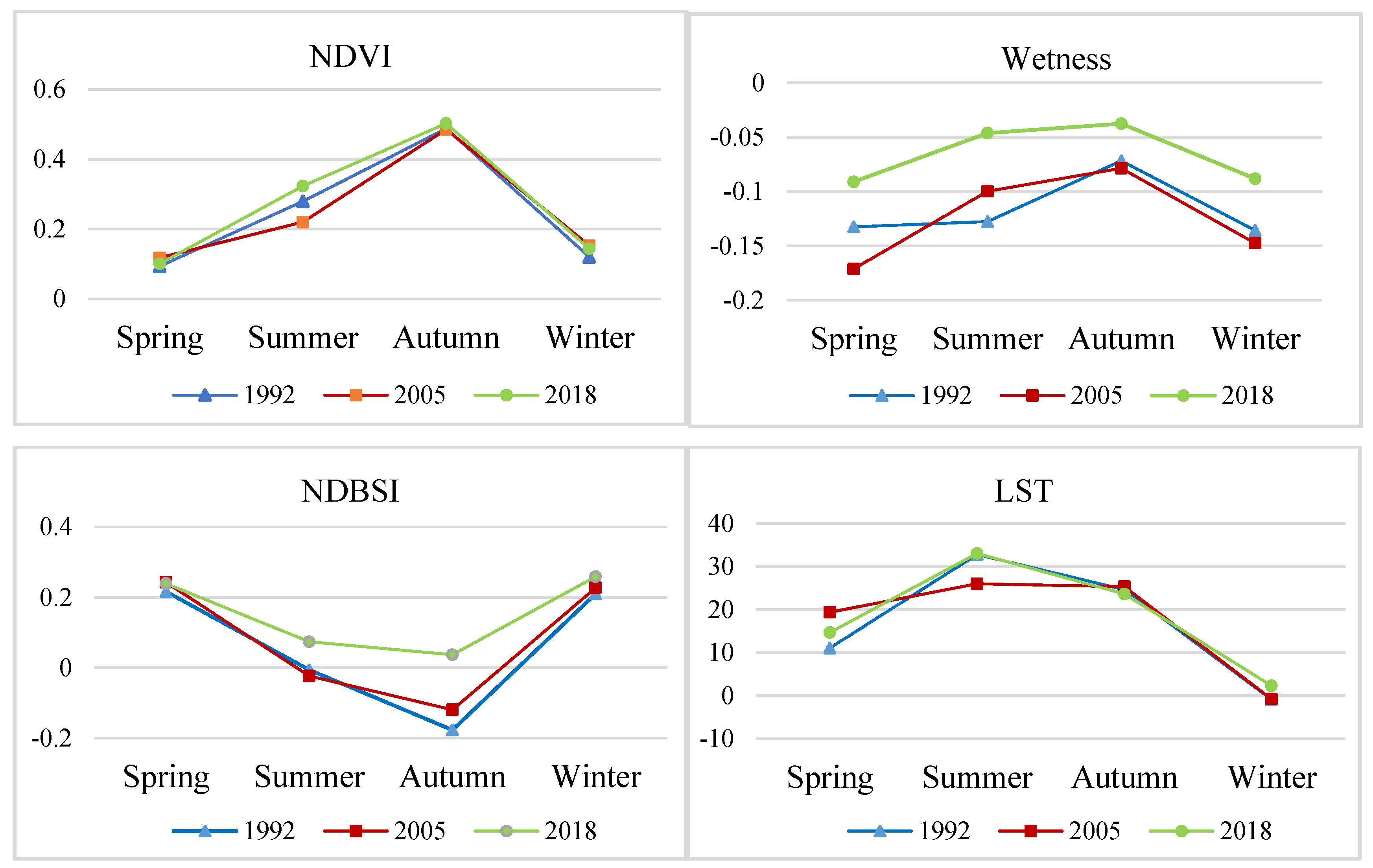
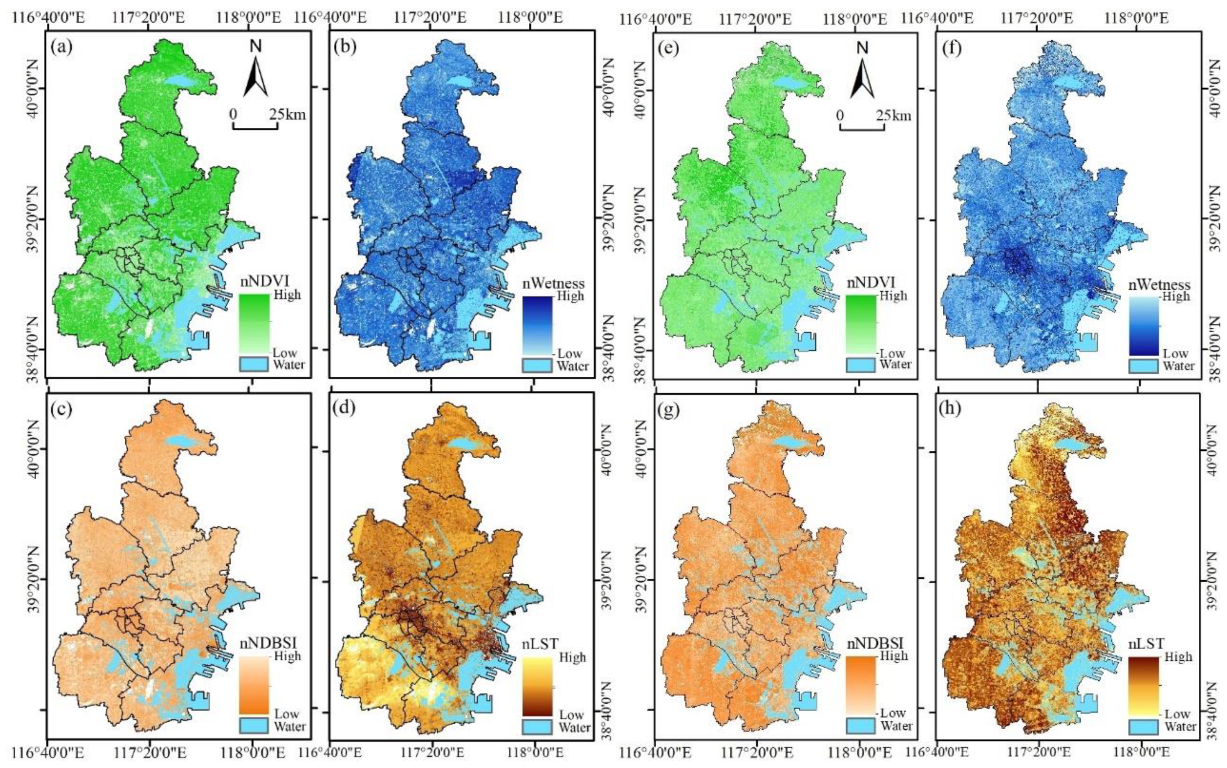
4.1. RSEI Indicators
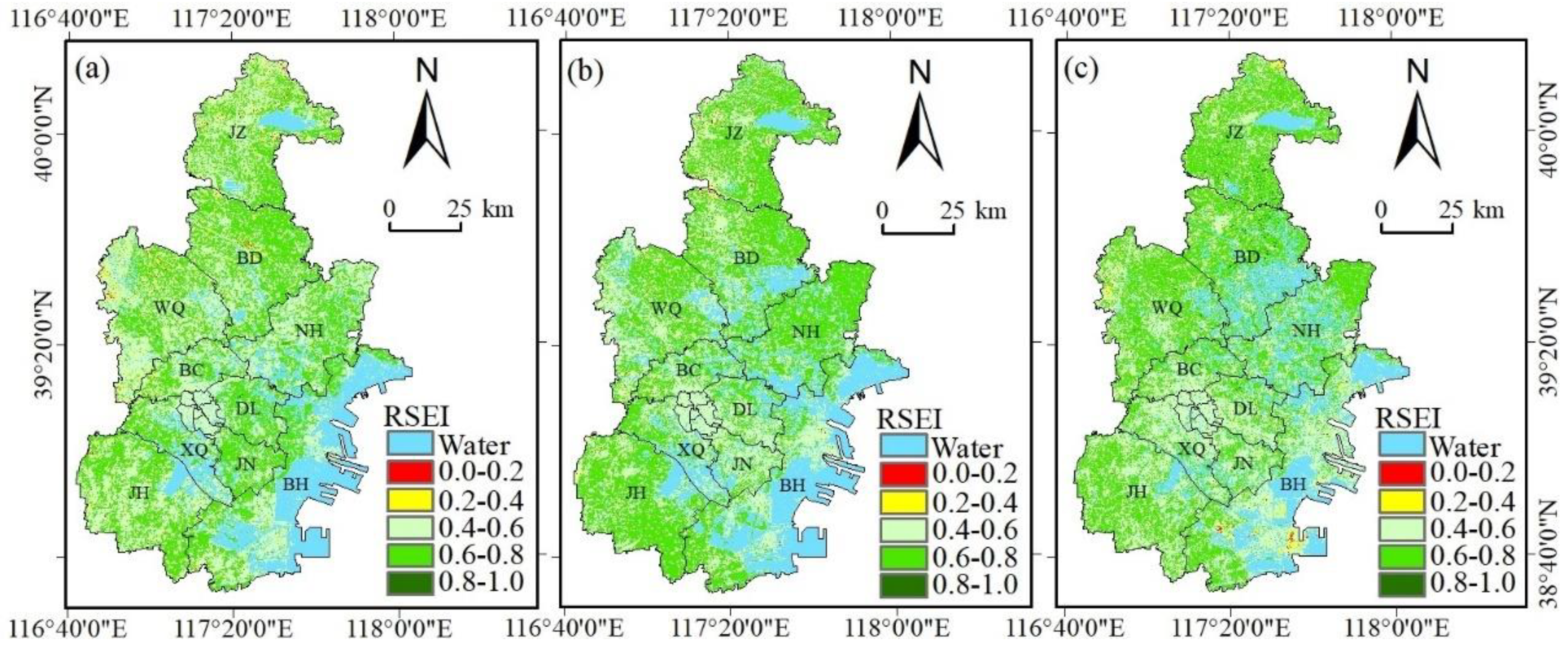
4.2. RSEI Distribution
4.3. RSEI Change
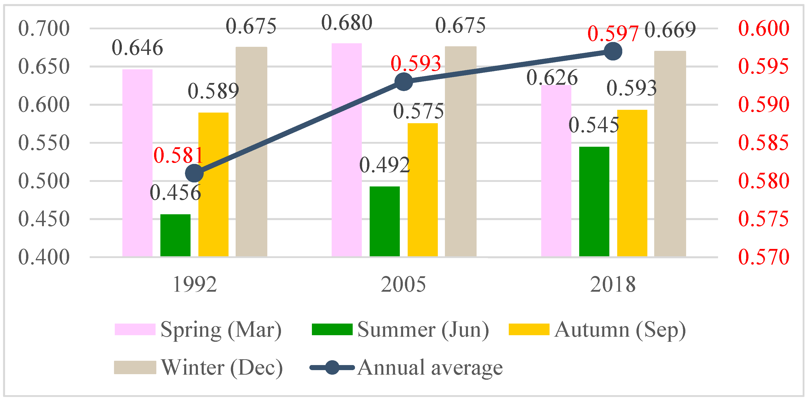
4.3.1. Seasonal and Annual RSEI Change
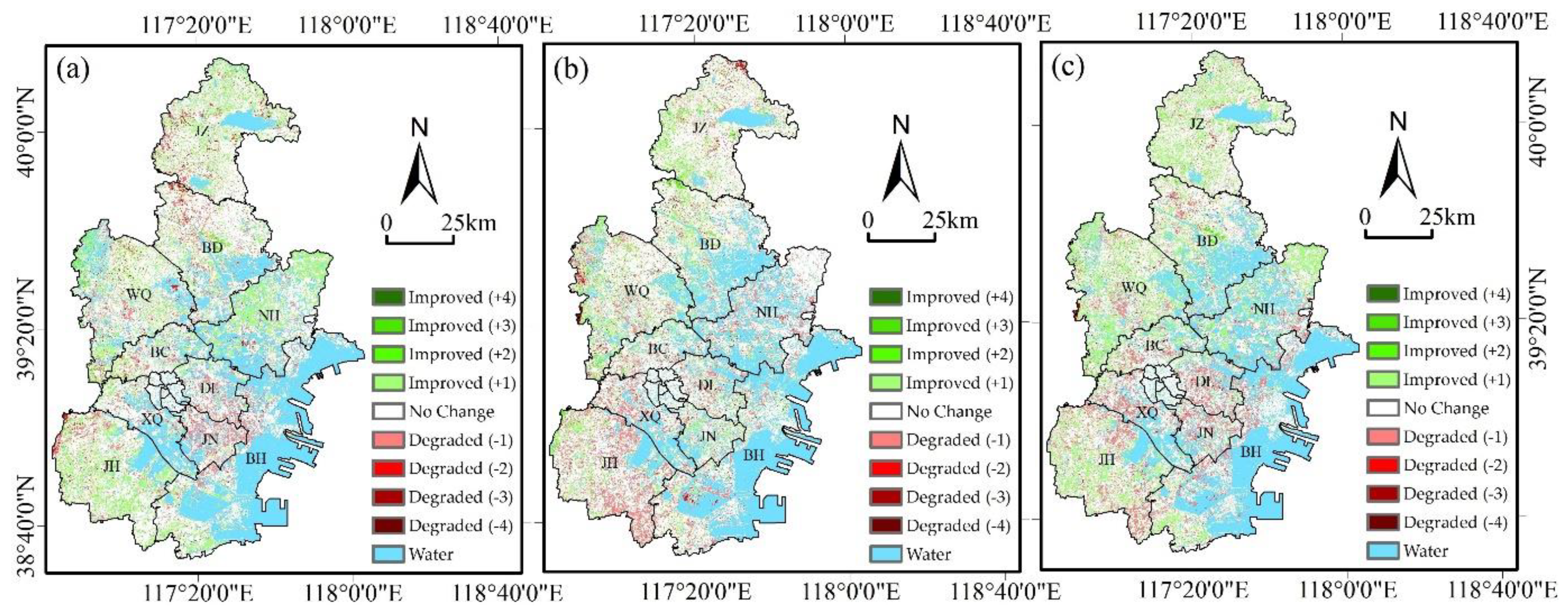
4.3.2. Spatial Distribution of RSEI Change
4.4. Innovations and Limitations
5. Conclusions
- Both the contributions of RSEI indicators to eco-environment quality and RSEI values vary with the season. Such seasonal variability should be considered normalizing indicator measures differently and using more remote-sensing images respectively to improve the assessment.
- Though with rapid urban expansion, Tianjin maintained a gradual urban eco-environment quality improvement over the 26 years from 1992 to 2018. This could be explained by the implementation of projects that increased urban green space.
- The most recent 13 years saw improved eco-environmental conditions in the joint area between the Central Urban Area and the Binhai New Area from eco-environmental restoration but these also gradually deteriorated in the Binhai New Area due to urban expansion and sea reclamation.
Author Contributions
Funding
Institutional Review Board Statement
Informed Consent Statement
Data Availability Statement
Acknowledgments
Conflicts of Interest
References
- Schneider, A. Monitoring land cover change in urban and peri-urban areas using dense time stacks of Landsat satellite data and a data mining approach. Remote Sens. Environ. 2012, 124, 689–704. [Google Scholar] [CrossRef]
- Wolch, J.R.; Byrne, J.; Newell, J.P. Urban green space, public health, and environmental justice: The challenge of making cities “just green enough.”. Landsc. Urban Plan. 2014, 125, 234–244. [Google Scholar] [CrossRef] [Green Version]
- Firozjaei, M.K.; Fathololomi, S.; Kiavarz, M.; Arsanjani, J.J.; Homaee, M.; Alavipanah, S.K. Modeling the impact of the COVID-19 lockdowns on urban surface ecological status: A case study of Milan and Wuhan cities. J. Environ. Manag. 2021, 286, 112236. [Google Scholar] [CrossRef]
- Li, Y.; Jia, L.; Wu, W.; Yan, J.; Liu, Y. Urbanization for rural sustainability—Rethinking China’s urbanization strategy. J. Clean. Prod. 2018, 178, 580–586. [Google Scholar] [CrossRef]
- Psomiadis, E.; Papazachariou, A.; Soulis, K.X.; Alexiou, D.S.; Charalampopoulos, I. Landslide mapping and susceptibility assessment using geospatial analysis and earth observation data. Land 2020, 9, 133. [Google Scholar] [CrossRef]
- Kouli, M.; Loupasakis, C.; Soupios, P.; Vallianatos, F. Landslide hazard zonation in high risk areas of Rethymno Prefecture, Crete Island, Greece. Nat. Hazards 2010, 52, 599–621. [Google Scholar] [CrossRef]
- Kumar, P.; Thakur, P.K.; Bansod, B.K.; Debnath, S.K. Multi-criteria evaluation of hydro-geological and anthropogenic parameters for the groundwater vulnerability assessment. Environ. Monit. Assess. 2017, 189, 564. [Google Scholar] [CrossRef]
- Willis, K.S. Remote sensing change detection for ecological monitoring in United States protected areas. Biol. Conserv. 2015, 182, 233–242. [Google Scholar] [CrossRef]
- He, F.; Gu, L.; Wang, T.; Zhang, Z. The synthetic geo-ecological environmental evaluation of a coastal coal-mining city using spatiotemporal big data: A case study in Longkou, China. J. Clean. Prod. 2017, 142, 854–866. [Google Scholar] [CrossRef]
- Li, S.; Bing, Z.; Jin, G. Spatially explicit mapping of soil conservation service in monetary units due to land use/cover change for the three gorges reservoir area, China. Remote Sens. 2019, 11, 468. [Google Scholar] [CrossRef] [Green Version]
- Zhang, L.; Liu, L.; Xia, Z.; Li, W.; Fan, Q. Sparse trajectory prediction based on multiple entropy measures. Entropy 2016, 18, 327. [Google Scholar] [CrossRef] [Green Version]
- Li, J.; Song, C.; Cao, L.; Zhu, F.; Meng, X.; Wu, J. Impacts of landscape structure on surface urban heat islands: A case study of Shanghai, China. Remote Sens. Environ. 2011, 115, 3249–3263. [Google Scholar] [CrossRef]
- Buyantuyev, A.; Wu, J. Urban heat islands and landscape heterogeneity: Linking spatiotemporal variations in surface temperatures to land-cover and socioeconomic patterns. Landsc. Ecol. 2010, 25, 17–33. [Google Scholar] [CrossRef]
- Xu, H.; Wang, M.; Shi, T.; Guan, H.; Fang, C.; Lin, Z. Prediction of ecological effects of potential population and impervious surface increases using a remote sensing based ecological index (RSEI). Ecol. Indic. 2018, 93, 730–740. [Google Scholar] [CrossRef]
- Xu, H.; Wang, Y.; Guan, H.; Shi, T.; Hu, X. Detecting ecological changes with a remote sensing based ecological index (RSEI) produced time series and change vector analysis. Remote Sens. 2019, 11, 2345. [Google Scholar] [CrossRef] [Green Version]
- Hu, X.; Xu, H. A new remote sensing index based on the pressure-state-response framework to assess regional ecological change. Environ. Sci. Pollut. Res. 2019, 26, 5381–5393. [Google Scholar] [CrossRef]
- Hu, X.; Xu, H. A new remote sensing index for assessing the spatial heterogeneity in urban ecological quality: A case from Fuzhou City, China. Ecol. Indic. 2018, 89, 11–21. [Google Scholar] [CrossRef]
- Shan, W.; Jin, X.; Ren, J.; Wang, Y.; Xu, Z.; Fan, Y.; Gu, Z.; Hong, C.; Lin, J.; Zhou, Y. Ecological environment quality assessment based on remote sensing data for land consolidation. J. Clean. Prod. 2019, 239, 118126. [Google Scholar] [CrossRef]
- Wen, X.; Ming, Y.; Gao, Y.; Hu, X. Dynamic monitoring and analysis of ecological quality of pingtan comprehensive experimental zone, a new type of sea island city, based on RSEI. Sustainability 2020, 12, 21. [Google Scholar] [CrossRef] [Green Version]
- Ji, J.; Wang, S.; Zhou, Y.; Liu, W.; Wang, L. Studying the Eco-Environmental Quality Variations of Jing-Jin-Ji Urban Agglomeration and Its Driving Factors in Different Ecosystem Service Regions from 2001 to 2015. IEEE Access 2020, 8, 154940–154952. [Google Scholar] [CrossRef]
- Zhou, Z.; Du, J.; Liu, Y. Evolution, development and evaluation of eco-transportation in Guangdong-Hong Kong-Macao Greater Bay Area. Syst. Sci. Control. Eng. 2020, 8, 97–107. [Google Scholar] [CrossRef]
- Wang, B.; Chen, L.; Li, L.; Xie, H.; Zhang, Y. Ecological response to land use change: A case study from the Chaohu lake basin, China. Bulg. Chem. Commun. 2017, 49, 200–206. [Google Scholar]
- Guo, B.; Fang, Y.; Jin, X.; Zhou, Y. Monitoring the effects of land consolidation on the ecological environmental quality based on remote sensing: A case study of Chaohu Lake Basin, China. Land Use Policy 2020, 95, 104569. [Google Scholar] [CrossRef]
- Li, Y.; Wu, L.; Han, Q.; Wang, X.; Zou, T.; Fan, C. Estimation of remote sensing based ecological index along the Grand Canal based on PCA-AHP-TOPSIS methodology. Ecol. Indic. 2021, 122, 107214. [Google Scholar] [CrossRef]
- Liao, W.; Jiang, W. Evaluation of the spatiotemporal variations in the eco-environmental quality in China based on the remote sensing ecological index. Remote Sens. 2020, 12, 2462. [Google Scholar] [CrossRef]
- Qureshi, S.; Alavipanah, S.K.; Konyushkova, M.; Mijani, N.; Fathololomi, S.; Firozjaei, M.K.; Homaee, M.; Hamzeh, S.; Kakroodi, A.A. A remotely sensed assessment of surface ecological change over the Gomishan Wetland, Iran. Remote Sens. 2020, 12, 2989. [Google Scholar] [CrossRef]
- Boori, M.S.; Choudhary, K.; Paringer, R.; Kupriyanov, A. Spatiotemporal ecological vulnerability analysis with statistical correlation based on satellite remote sensing in Samara, Russia. J. Environ. Manag. 2021, 285, 112138. [Google Scholar] [CrossRef]
- Firozjaei, M.K.; Kiavarz, M.; Homaee, M.; Arsanjani, J.J.; Alavipanah, S.K. A novel method to quantify urban surface ecological poorness zone: A case study of several European cities. Sci. Total Environ. 2021, 757, 143755. [Google Scholar] [CrossRef]
- Karimi Firozjaei, M.; Fathololoumi, S.; Kiavarz, M.; Biswas, A.; Homaee, M.; Alavipanah, S.K. Land Surface Ecological Status Composition Index (LSESCI): A novel remote sensing-based technique for modeling land surface ecological status. Ecol. Indic. 2021, 123, 107375. [Google Scholar] [CrossRef]
- Yue, H.; Liu, Y.; Li, Y.; Lu, Y. Eco-environmental quality assessment in china’s 35 major cities based on remote sensing ecological index. IEEE Access 2019, 7, 51295–51311. [Google Scholar] [CrossRef]
- Seddon, A.W.R.; Macias-Fauria, M.; Long, P.R.; Benz, D.; Willis, K.J. Sensitivity of global terrestrial ecosystems to climate variability. Nature 2016, 531, 229–232. [Google Scholar] [CrossRef] [Green Version]
- Tianjin Weather. Available online: https://weather.cma.cn/web/weather/54517 (accessed on 11 May 2021).
- Yi, P.; Li, W.; Zhang, D. Sustainability assessment and key factors identification of first-tier cities in China. J. Clean. Prod. 2021, 281, 125369. [Google Scholar] [CrossRef]
- 2019 Official List of New First-Tier Cities: Where Does Your City Rank? Available online: https://www.yicai.com/news/100200192.html (accessed on 11 May 2021).
- Tianjin Municipal People’s Government. Tianjin Economic Yearbook 1992, 1st ed.; Tianjin Statistical Yearbooks Press: Tianjin, China, 1992; p. 700. [Google Scholar]
- Tianjin Municipal People’s Government. Yearbook of Tianjin 2019, 1st ed.; Tianjin Statistical Yearbooks Press: Tianjin, China, 2019; p. 50. [Google Scholar]
- Yue, S.; Yang, Y.; Pu, Z. Total-factor ecology efficiency of regions in China. Ecol. Indic. 2017, 73, 284–292. [Google Scholar] [CrossRef]
- Mishra, N.; Haque, M.O.; Leigh, L.; Aaron, D.; Helder, D.; Markham, B. Radiometric cross calibration of landsat 8 Operational Land Imager (OLI) and landsat 7 enhanced thematic mapper plus (ETM+). Remote Sens. 2014, 6, 12619–12638. [Google Scholar] [CrossRef] [Green Version]
- Koutsias, N.; Pleniou, M. Comparing the spectral signal of burned surfaces between Landsat 7 ETM+ and Landsat 8 OLI sensors. Int. J. Remote Sens. 2015, 36, 3714–3732. [Google Scholar] [CrossRef]
- Rouse, J.W.; Haas, R.H.; Scheel, J.A.; Deering, D.W. Monitoring Vegetation Systems in the Great Plains with ERTS. Proc. Third ERTS Symp. 1973, 1, 48–62. [Google Scholar]
- Li, L.; Bakelants, L.; Solana, C.; Canters, F.; Kervyn, M. Dating lava flows of tropical volcanoes by means of spatial modeling of vegetation recovery. Earth Surf. Process. Landf. 2018, 43, 840–856. [Google Scholar] [CrossRef]
- Zhou, X.; Li, L.; Chen, L.; Liu, Y.; Cui, Y.; Zhang, Y.; Zhang, T. Discriminating urban forest types from Sentinel-2A image data through linear spectral mixture analysis: A case study of Xuzhou, East China. Forests 2019, 10, 478. [Google Scholar] [CrossRef] [Green Version]
- Li, L.; Zhou, X.; Chen, L.; Chen, L.; Zhang, Y.; Liu, Y. Estimating urban vegetation biomass from sentinel-2A image data. Forests 2020, 11, 125. [Google Scholar] [CrossRef] [Green Version]
- Crist, E.P. A TM Tasseled Cap equivalent transformation for reflectance factor data. Remote Sens. Environ. 1985, 17, 301–306. [Google Scholar] [CrossRef]
- Baig, M.H.A.; Zhang, L.; Shuai, T.; Tong, Q. Derivation of a tasselled cap transformation based on Landsat 8 at-satellite reflectance. Remote Sens. Lett. 2014, 5, 423–431. [Google Scholar] [CrossRef]
- Xu, H. A new index for delineating built-up land features in satellite imagery. Int. J. Remote Sens. 2008, 29, 4269–4276. [Google Scholar] [CrossRef]
- Essa, W.; Verbeiren, B.; van der Kwast, J.; Van de Voorde, T.; Batelaan, O. Evaluation of the DisTrad thermal sharpening methodology for urban areas. Int. J. Appl. Earth Obs. Geoinf. 2012, 19, 163–172. [Google Scholar] [CrossRef]
- Jimenez-Munoz, J.C.; Cristobal, J.; Sobrino, J.A.; Sòria, G.; Ninyerola, M.; Pons, X. Revision of the single-channel algorithm for land surface temperature retrieval from landsat thermal-infrared data. IEEE Trans. Geosci. Remote Sens. 2009, 47, 339–349. [Google Scholar] [CrossRef]
- Sobrino, J.A.; Jiménez-Muñoz, J.C.; Paolini, L. Land surface temperature retrieval from LANDSAT TM 5. Remote Sens. Environ. 2004, 90, 434–440. [Google Scholar] [CrossRef]
- Weng, Q. Thermal infrared remote sensing for urban climate and environmental studies: Methods, applications, and trends. ISPRS J. Photogramm. Remote Sens. 2009, 64, 335–344. [Google Scholar] [CrossRef]
- Nichol, J. Remote sensing of urban heat islands by day and night. Photogramm. Eng. Remote Sens. 2005, 71, 613–621. [Google Scholar] [CrossRef]
- Liu, W.; Li, L.; Chen, L.; Wen, M.; Wang, J.; Yuan, L.; Liu, Y.; Li, H. Testing a comprehensive volcanic risk assessment of tenerife by volcanic hazard simulations and social vulnerability analysis. ISPRS Int. J. Geo-Inf. 2020, 9, 273. [Google Scholar] [CrossRef]
- Yang, C.; Zeng, W.; Yang, X. Coupling coordination evaluation and sustainable development pattern of geo-ecological environment and urbanization in Chongqing municipality, China. Sustain. Cities Soc. 2020, 61, 102271. [Google Scholar] [CrossRef]
- Mostafiz, C.; Chang, N.-B. Tasseled cap transformation for assessing hurricane landfall impact on a coastal watershed. Int. J. Appl. Earth Obs. Geoinf. 2018, 73, 736–745. [Google Scholar] [CrossRef]
- Yuan, B.; Fu, L.; Zou, Y.; Zhang, S.; Chen, X.; Li, F.; Deng, Z.; Xie, Y. Spatiotemporal change detection of ecological quality and the associated affecting factors in Dongting Lake Basin, based on RSEI. J. Clean. Prod. 2021, 302, 126995. [Google Scholar] [CrossRef]
- Sun, X.; Tan, X.; Chen, K.; Song, S.; Zhu, X.; Hou, D. Quantifying landscape-metrics impacts on urban green-spaces and water-bodies cooling effect: The study of Nanjing, China. Urban For. Urban Green. 2020, 55, 126838. [Google Scholar] [CrossRef]
- Jensen, J.R. Remote Sensing of the Environment. In Remote Sensing of the Environment: Pearson New International Edition: An Earth Resource Perspective, 2nd ed.; Pearson Education Limited: Essex, UK, 2013; pp. 17–19. [Google Scholar]
- Cui, Y.; Li, L.; Chen, L.; Zhang, Y.; Cheng, L.; Zhou, X.; Yang, X. Land-use carbon emissions estimation for the Yangtze River Delta Urban Agglomeration using 1994-2016 Landsat image data. Remote Sens. 2018, 10, 1334. [Google Scholar] [CrossRef] [Green Version]
- Li, H.; Li, L.; Chen, L.; Zhou, X.; Cui, Y.; Liu, Y.; Liu, W. Mapping and characterizing spatiotemporal dynamics of impervious surfaces using landsat images: A case study of Xuzhou, East China from 1995 to 2018. Sustainability 2019, 11, 1224. [Google Scholar] [CrossRef] [Green Version]
- Hu, S.; Chen, L.; Li, L.; Zhang, T.; Yuan, L.; Cheng, L.; Wang, J.; Wen, M. Simulation of land use change and ecosystem service value dynamics under ecological constraints in Anhui province, China. Int. J. Environ. Res. Public Health 2020, 17, 4228. [Google Scholar] [CrossRef] [PubMed]
- Yunus, A.P.; Fan, X.; Tang, X.; Jie, D.; Xu, Q.; Huang, R. Decadal vegetation succession from MODIS reveals the spatio-temporal evolution of post-seismic landsliding after the 2008 Wenchuan earthquake. Remote Sens. Environ. 2020, 236, 111476. [Google Scholar] [CrossRef]
- Wu, W.; Zhao, S.; Zhu, C.; Jiang, J. A comparative study of urban expansion in Beijing, Tianjin and Shijiazhuang over the past three decades. Landsc. Urban Plan. 2015, 134, 93–106. [Google Scholar] [CrossRef]
- The Two-City Green Space Ecological Barrier Project Is Taking Shape. Available online: http://www.tj.gov.cn/sy/zwdt/bmdt/202007/t20200730_3236789.html (accessed on 11 May 2021).


| Area | District |
|---|---|
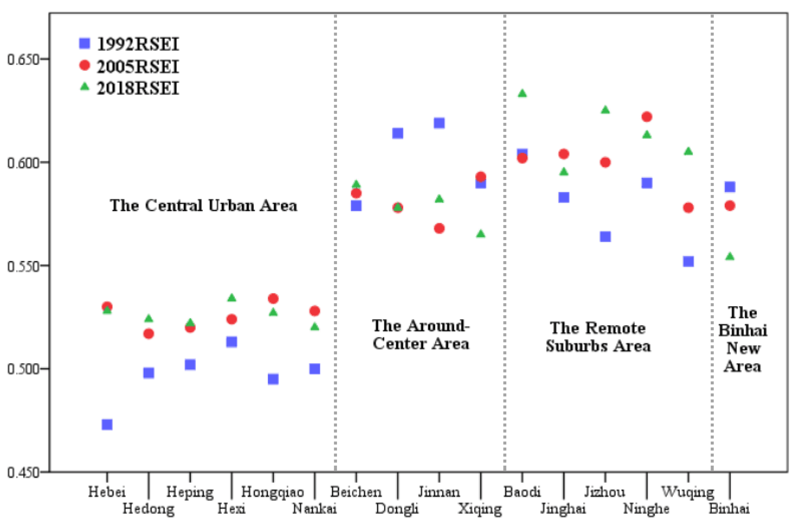
| The Central Urban Area | Heping (HP), Hongqiao (HQ), Hebei (HB), Hexi (HX), Hedong (HD), Nankai (NK) |
| The Around-Center Area | Jinnan (JN), Dongli (DL), Beichen (BC), Xiqing (XQ) |
| The Binhai New Area | Binhaixinqu (BH) |
| The Remote Suburbs Area | Ninghe (NH), Jinghai (JH), Baodi (BD),Wuqing (WQ), Jizhou (JZ) |
| Year | Season | Path | Row | Imaging Date |
|---|---|---|---|---|
| 1991/ 1992/ 1993 | Spring | 122 | 32/33 | 22 March 1991 |
| 123 | 32/33 | 13 March 1991 | ||
| Summer | 122 | 32/33 | 27 May 1992 | |
| Autumn | 122 | 32/33 | 3 September 1993 | |
| 123 | 32/33 | 25 August 1993 | ||
| Winter | 122 | 32/33 | 21 December 1992 | |
| 123 | 32/33 | 28 December 1992 | ||
| 2004/ 2005/ 2006 | Spring | 122 | 32/33 | 28 March 2005 |
| 123 | 32/33 | 19 March 2005 | ||
| Summer | 122 | 32/33 | 28 May 2004 | |
| 123 | 32/33 | 19 May 2004 | ||
| Autumn | 122 | 32/33 | 4 September 2005 | |
| Winter | 122 | 32/33 | 28 December 2006 | |
| 2018 | Spring | 122 | 32/33 | 16 March 2018 |
| 123 | 32/33 | 8 April 2018 | ||
| Summer | 122 | 32/33 | 4 June 2018 | |
| 123 | 32/33 | 27 June 2018 | ||
| Autumn | 122 | 32/33 | 24 September 2018 | |
| 123 | 32/33 | 1 October 2018 | ||
| Winter | 122 | 32/33 | 13 December 2018 | |
| 123 | 32/33 | 4 December 2018 |
| Year | Measure | Spring | Summer | Autumn | Winter |
|---|---|---|---|---|---|
| 1992 | Wetness | −0.297 | 0.391 | 0.231 | −0.405 |
| NDBSI | 0.161 | −0.660 | −0.742 | 0.264 | |
| LST | 0.062 | −0.439 | −0.624 | 0.251 | |
| 2005 | Wetness | −0.276 | 0.503 | 0.327 | −0.221 |
| NDBSI | 0.302 | −0.826 | −0.701 | 0.082 | |
| LST | 0.140 | −0.497 | −0.357 | 0.177 | |
| 2018 | Wetness | −0.339 | 0.617 | 0.322 | −0.101 |
| NDBSI | 0.377 | −0.808 | −0.457 | 0.018 | |
| LST | 0.024 | −0.432 | −0.518 | 0.221 |
| RSEI Grade | 1992 | 2005 | 2018 | |||
|---|---|---|---|---|---|---|
| Area/km2 | % | Area/km2 | % | Area/km2 | % | |
| Poor (0–0.2) | 36.5 | 0.380 | 24.6 | 0.271 | 30.9 | 0.328 |
| Fair (0.2–0.4) | 256.9 | 2.670 | 205.9 | 2.264 | 189.1 | 2.007 |
| Moderate (0.4–0.6) | 5124.7 | 53.271 | 4057.5 | 44.613 | 4501.9 | 47.773 |
| Good (0.6–0.8) | 4199.9 | 43.658 | 4806.6 | 52.850 | 4671.4 | 49.571 |
| Excellent (0.8–1) | 2.0 | 0.022 | 0.2 | 0.002 | 30.3 | 0.321 |
| Total | 9620.03 | 100 | 9094.79 | 100 | 9423.66 | 100 |
| Class | Change | 1992–2005 | 2005–2018 | 1992–2018 | |||
|---|---|---|---|---|---|---|---|
| Class Area/km2 | Change Area/km2 | Class Area/km2 | Change Area/km2 | Class Area/km2 | Change Area/km2 | ||
| Degraded | −4 | 1082.63 (12.61%) | 1.23 | 1404.46 (17.00%) | 6.15 | 1347.42 (16.02%) | 1.10 |
| −3 | 19.22 | 31.64 | 15.88 | ||||
| −2 | 144.85 | 117.98 | 98.46 | ||||
| −1 | 917.32 | 1248.70 | 2108.88 | ||||
| No change | 0 | 5521.98 (64.31%) | 5521.98 | 5410.78 (65.50%) | 5410.78 | 4838.96 (57.53%) | 4838.96 |
| Improved | 1 | 1981.43 (23.08%) | 1764.56 | 1445.25 (17.50%) | 1246.93 | 2224.32 (26.45%) | 1274.81 |
| 2 | 189.78 | 175.03 | 45.35 | ||||
| 3 | 26.67 | 22.65 | 20.62 | ||||
| 4 | 0.42 | 0.63 | 6.64 | ||||
Publisher’s Note: MDPI stays neutral with regard to jurisdictional claims in published maps and institutional affiliations. |
© 2021 by the authors. Licensee MDPI, Basel, Switzerland. This article is an open access article distributed under the terms and conditions of the Creative Commons Attribution (CC BY) license (https://creativecommons.org/licenses/by/4.0/).
Share and Cite
Zhang, T.; Yang, R.; Yang, Y.; Li, L.; Chen, L. Assessing the Urban Eco-Environmental Quality by the Remote-Sensing Ecological Index: Application to Tianjin, North China. ISPRS Int. J. Geo-Inf. 2021, 10, 475. https://0-doi-org.brum.beds.ac.uk/10.3390/ijgi10070475
Zhang T, Yang R, Yang Y, Li L, Chen L. Assessing the Urban Eco-Environmental Quality by the Remote-Sensing Ecological Index: Application to Tianjin, North China. ISPRS International Journal of Geo-Information. 2021; 10(7):475. https://0-doi-org.brum.beds.ac.uk/10.3390/ijgi10070475
Chicago/Turabian StyleZhang, Ting, Ruiqing Yang, Yibo Yang, Long Li, and Longqian Chen. 2021. "Assessing the Urban Eco-Environmental Quality by the Remote-Sensing Ecological Index: Application to Tianjin, North China" ISPRS International Journal of Geo-Information 10, no. 7: 475. https://0-doi-org.brum.beds.ac.uk/10.3390/ijgi10070475