
Investigating Eco-Environmental Vulnerability for China–Pakistan Economic Corridor Key Sector Punjab Using Multi-Sources Geo-Information


Abstract
:1. Introduction
2. Materials and Methods
2.1. The Study Area
2.2. Data Sources
- Landsat 8 OLI/TIRS imagery;
- Meteorological data;
- Internationally accepted GIS data exchange portals;
- Official reports of the Government of Pakistan (GOP);
- Digital elevation model (DEM) data;
- High-resolution imagery of Google Earth.
2.3. Data Processing
2.4. Methodology
Explanation of Best–Worst Method (BWM)
3. Results
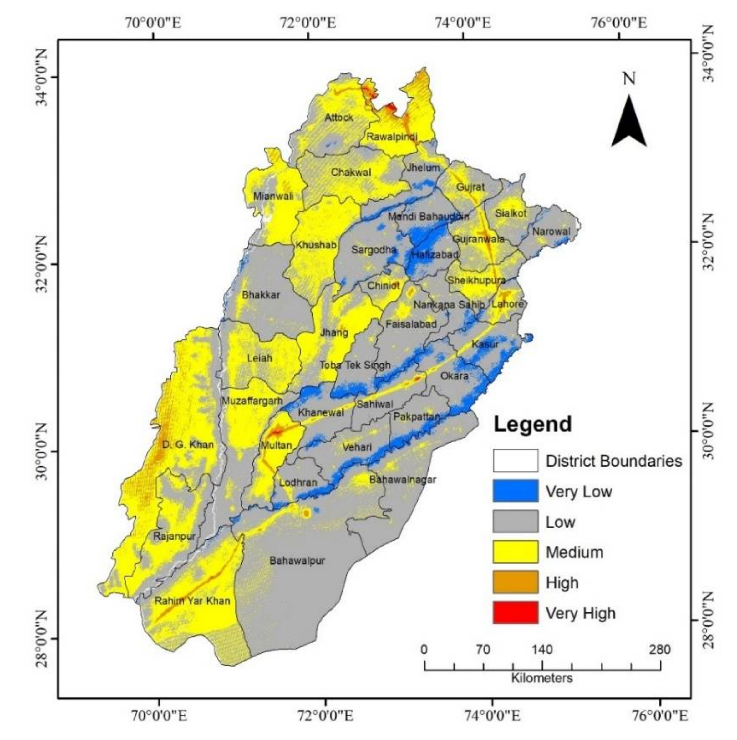
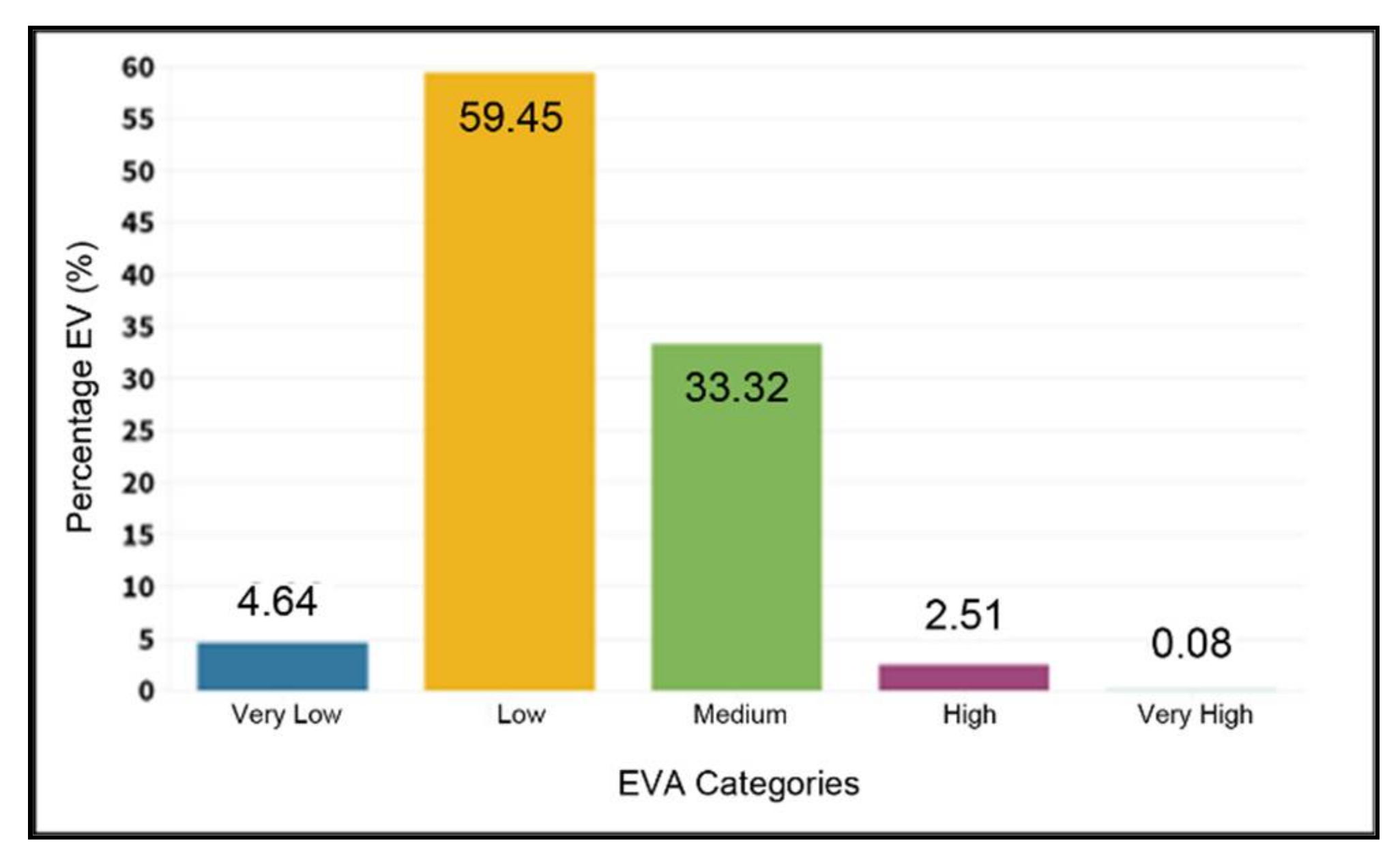
3.1. Overall Interpretation of EVA Results
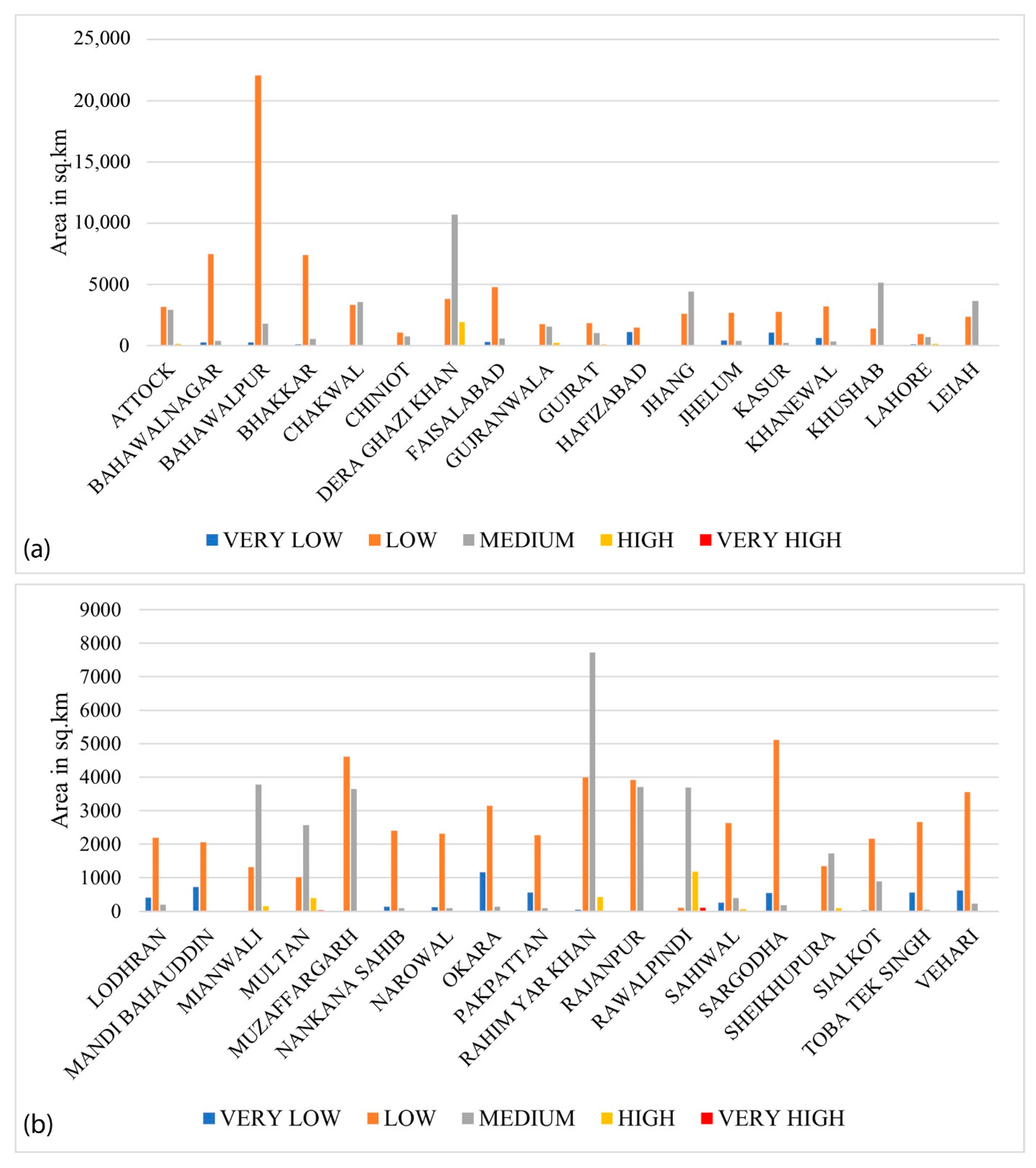
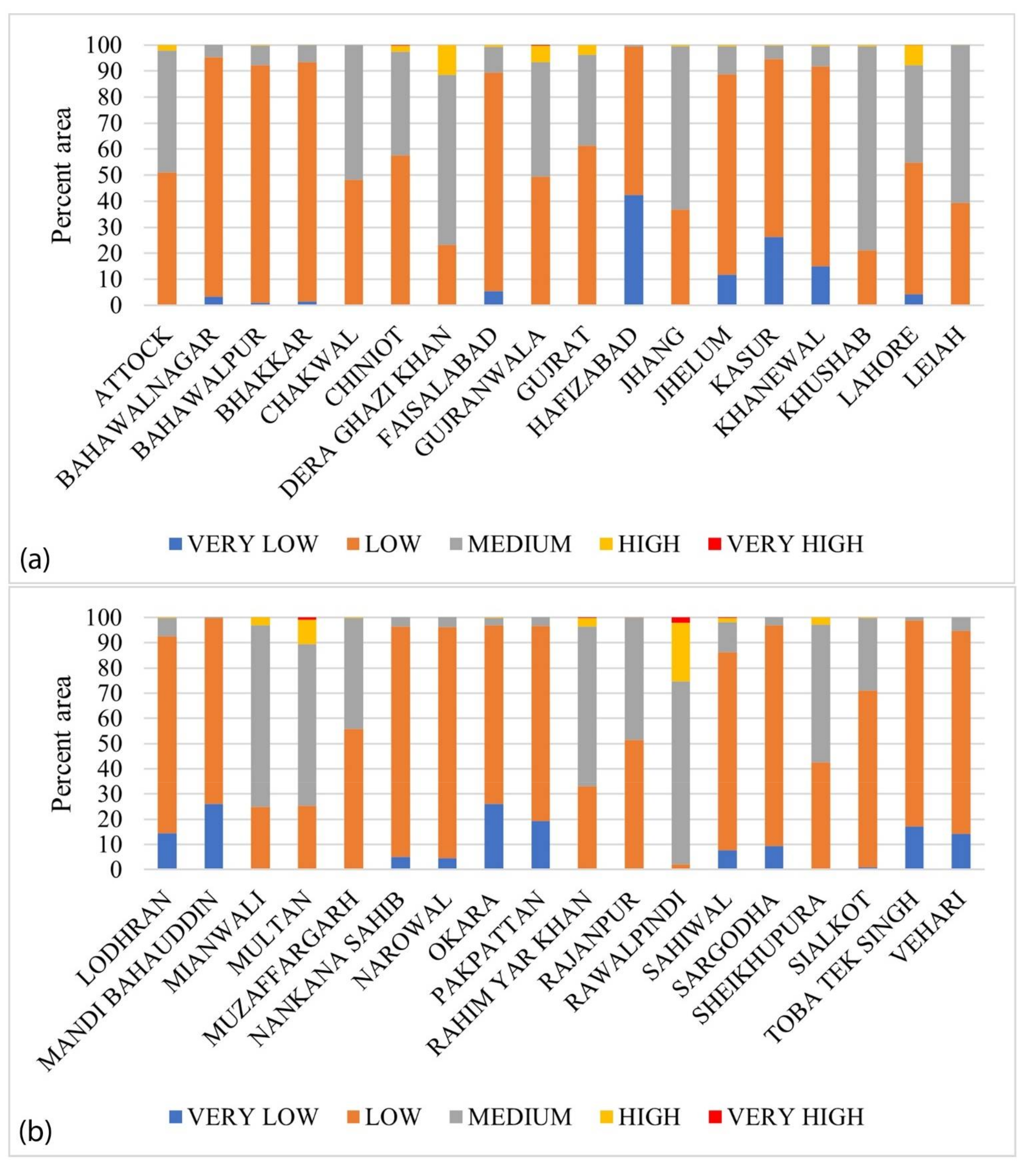
3.2. District Wise Comparison of EVA Results
4. Discussion
4.1. Significance of the Study and EVA Framework
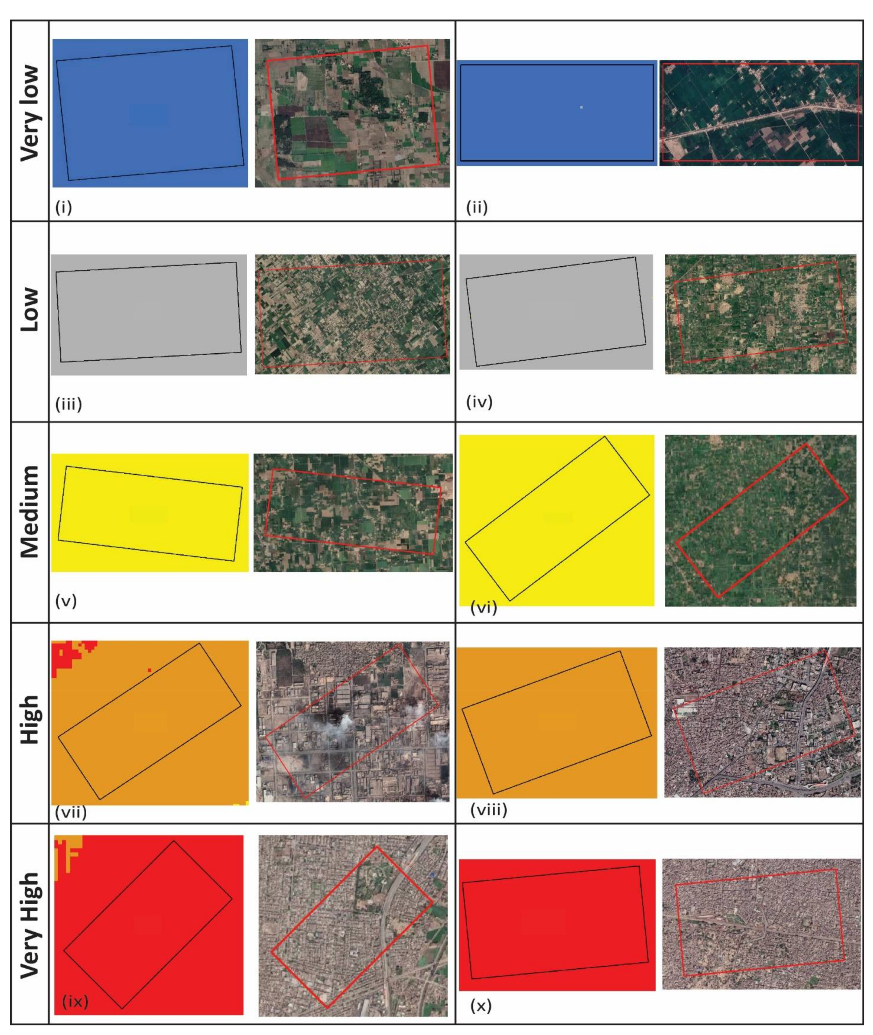
4.2. Validation
4.3. Proposed Actions for Protecting the Eco-Environment of the Region
4.4. Prospects of the Study
5. Conclusions
Author Contributions
Funding
Data Availability Statement
Acknowledgments
Conflicts of Interest
Appendix A


| Hydrometeorology (G1) | Socio-economics (G2) | Land Resources (G3) | Topography (G4) | Hazards (G5) | CPEC Projects (G6) | |||||||||||||||||
|---|---|---|---|---|---|---|---|---|---|---|---|---|---|---|---|---|---|---|---|---|---|---|
| j1 | j2 | j3 | j4 | j5 | j6 | j7 | j8 | j9 | j10 | j11 | j12 | j13 | j14 | j15 | j16 | j17 | j18 | j19 | j20 | j21 | j22 | Index |
| value | value | meter | °C | mm | value | people.sqkm | meter | meter | meter | value | description | ° angle | meter | degree | description | description | description | meter | meter | meter | meter | no units |
| No Data | No Data | No Data | No Data | No Data | No Data | No Data | No Data | No Data | No Data | No Data | No Data | No Data | No Data | No Data | No Data | No Data | No Data | 4000.01–261,643.781 | 1000.01–312,381.25 | 3000.01–215,535.672 | 500.01–215,535 | 0 |
| 0.6–0.942 | −0.768–0.024 | 0–400 | 14.95–16.906 | 14.5–26.896 | −0.98–(−0.52) | 0.006–2.743 | 30,000.01–97,583.297 | 130,000.01–140,910 | 17,000.01–138,078 | 0.466–0.811 | Irrigated croplands and built-up areas | 0–1.61 | 0–1.61 | Flat (−1–0) | Very low | Very low | Very low | 3500.01–4000 | 500.01–1000 | 2500.01–3000 | 400.01–500 | 1 |
| 0.332–0.6 | 0.024–0.209 | 400.01–1200 | 16.906–18.091 | 26.896–37.676 | −0.52–0.378 | 2.743–9.131 | 18,000.01–30,000 | 100,000.01–1,300,000 | 10,000.01–17,000 | 0.329–0.466 | Rainfed croplands and irrigated croplands | 1.62–5.79 | 1.62–5.79 | North (0–22.5) | - | - | - | 3000.01–3500 | - | 2000.01–2500 | 300.01–400 | 2 |
| - | - | 1200.01–2500 | 18.091–19.082 | 37.676–52.767 | - | 9.131–20.08 | 14,000.01–18,000 | 70,000.01–100,000 | 7000.01–10,000 | - | Irrigated croplands and bare areas | 5.8–12.22 | 5.8–12.22 | Northeast (22.5–67.5) | Low | Low | Low | 2500.01–3000 | - | 1500.01–2000 | 200.01–300 | 3 |
| - | 0.209–0.301 | 2500.01–4000 | - | 52.767–70.554 | −0.378–0 | 20.08–36.505 | 10,000.01–14,000 | 20,000.01–70,000 | 5000.01–7000 | 0.18–0.329 | Irrigated croplands and vegetation | 12.23–21.51 | 12.23–21.51 | East (67.5–112.5) | - | - | - | 2000.01–2500 | - | 1000.01–1500 | 100.01–200 | 4 |
| 0.107–0.332 | - | 4000.01–8000 | - | 70.554–86.723 | - | 36.505–60.229 | 6000.01–10,000 | 15,000.01–20,000 | 3000.01–5000 | −0.01–0.18 | Rainfed croplands and vegetation | 21.55–32.15 | 21.55–32.15 | Southeast (112.5–157.5) | Medium | Medium | Medium | 1500.01–2000 | - | - | - | 5 |
| - | 0.301–0.393 | 8000.01–10,000 | 19.082–19.909 | 86.723–101.275 | 0–0.4 | 60.229–90.34 | 4000.01–6000 | 10,000.01–15,000 | 1500.01–3000 | - | Bare areas & cropland vegetation | 32.16–43.08 | 32.16–43.08 | South (157.5–202.5) | - | - | - | 1000.01–1500 | - | - | - | 6 |
| −0.017–(0.107) | - | 10,000.01–130,000 | - | 101.275–119.6 | - | 90.34–136.876 | 2500.01–4000 | 5000.01–10,000 | 500.01–1500 | −0.706–0.01 | Bare areas and sparse vegetation | 43.09–54.97 | 43.09–54.97 | Southwest (202.5–247.5) West (247.5–292.5) | High | High | High | 500.01–1000 | - | 500.01–1000 | - | 7 |
| −0.568–(−0.017) | 0.393–0.7 | 13,000.01–153,633.078 | 19.909–21.975 | 119.6–151.939 | 0.4–0.824 | 136.876–232.685 | 0–2500 | 0–5000 | 0–500 | - | - | 54.98–81.98 | 54.98–81.98 | Northwest (292.5–337.5) North (337.5–360) | Very High | Very High | Very High | 0–500 | 0–500 | 0–500 | 0–100 | 8 |
References
- Liu, W. Scientific understanding of the Belt and Road Initiative of China and related research themes. Prog. Geogr. 2015, 34, 538. [Google Scholar]
- Kanwal, S.; Pitafi, A.H.; Ahmad, M.; Khan, N.A.; Ali, S.M.; Surahio, M.K. Cross-border analysis of China—Pakistan Economic Corridor development project and local residence quality of life. J. Public Aff. 2020, 20, e2022. [Google Scholar] [CrossRef]
- Makhdoom, A.S.; Shah, A.B.; Sami, K. Pakistan on the roadway to socio-economic development: A comprehensive study of China Pakistan Economic Corridor (CPEC). Gov. Annu. Res. J. Polit. Sci. 2018, 6, 6. [Google Scholar]
- Liu, N. Will China build a green belt and road in the arctic? Rev. Eur. Comp. Int. Environ. Law 2018, 27, 55–62. [Google Scholar] [CrossRef]
- Suocheng, D.; Kolosov, V.; Yu, L.; Zehong, L.; Fujia, L.; Minyan, Z.; Guangyi, S.; Huilu, Y.; Hao, C.; Peng, G. Green Development Modes of the Belt and Road. Geogr. Environ. Sustain. 2017, 10, 53–69. [Google Scholar] [CrossRef]
- Greening the CPEC: China to Turn CPEC into a Blueprint of a Green Initiative—China Pakistan Economic Corridor. Available online: http://cpecinfo.com/greening-the-cpec-china-to-turn-cpec-into-a-blueprint-of-a-green-initiative/ (accessed on 18 January 2021).
- Ibrar, M.; Mi, J.; Rafiq, M. China Pakistan Economic Corridor: Socio-cultural Cooperation and its Impact on Pakistan. In Proceedings of the 5th EEM international conference on education science and social science (EEM-ESSS 2016), Sydney, Australia, 24–25 December 2016. [Google Scholar]
- Kamran, A.; Syed, N.A.; Rizvi, S.M.A.; Ameen, B.; Ali, S.N. Advances in Intelligent Systems and Computing. In Impact of China-Pakistan Economic Corridor (CPEC) on Agricultural Sector of Pakistan; Springer: Cham, Switzerland, 2021; Volume 1191 AISC, p. 594. [Google Scholar]
- Wolf, S.O. China-Pakistan Economic Corridor (CPEC) and Its Impact on Gilgit-Baltistan; South Asia Democratic Forum (SADF): Brussels, Belgium, 2016. [Google Scholar]
- Abalakov, A.D.; Lopatkin, D.A.; Novikova, L.S. Stability of landscapes in the areas of creation of economic corridors “China-Mongolia-Russia”. IOP Conf. Ser. Earth Environ. Sci. 2018, 190, 012022. [Google Scholar] [CrossRef]
- Li, D.; Shangguan, D.; Anjum, M.N. Glacial Lake Inventory Derived from Landsat 8 OLI in 2016–2018 in China–Pakistan Economic Corridor. ISPRS Int. J. Geo-Inf. 2020, 9, 294. [Google Scholar] [CrossRef]
- Ahmad, H.; Ningsheng, C.; Rahman, M.; Islam, M.M.; Pourghasemi, H.R.; Hussain, S.F.; Habumugisha, J.M.; Liu, E.; Zheng, H.; Ni, H.; et al. Geohazards Susceptibility Assessment along the Upper Indus Basin Using Four Machine Learning and Statistical Models. ISPRS Int. J. Geo-Inf. 2021, 10, 315. [Google Scholar] [CrossRef]
- Zeng, D.; Wu, J.; Mu, Y.; Deng, M.; Wei, Y.; Sun, W. Spatial-Temporal Pattern Changes of UTCI in the China-Pakistan Economic Corridor in Recent 40 Years. Atmosphere 2020, 11, 858. [Google Scholar] [CrossRef]
- Hassan, J.; Chen, X.; Kayastha, R.B.; Nie, Y. Multi-model assessment of glacio-hydrological changes in central Karakoram, Pakistan. J. Mt. Sci. 2021, 18, 1995–2011. [Google Scholar] [CrossRef]
- Ullah, S.; You, Q.; Ullah, W.; Ali, A. Observed changes in precipitation in China-Pakistan economic corridor during 1980–2016. Atmos. Res. 2018, 210, 1–14. [Google Scholar] [CrossRef]
- Eck, M.A.; Murray, A.R.; Ward, A.R.; Konrad, C.E. Influence of growing season temperature and precipitation anomalies on crop yield in the southeastern United States. Agric. For. Meteorol. 2020, 291, 108053. [Google Scholar] [CrossRef]
- Guo, E.; Wang, Y.; Jirigala, B.; Jin, E. Spatiotemporal variations of precipitation concentration and their potential links to drought in mainland China. J. Clean. Prod. 2020, 267, 122004. [Google Scholar]
- Huangpeng, Q.; Huang, W.; Gholinia, F. Forecast of the hydropower generation under influence of climate change based on RCPs and Developed Crow Search Optimization Algorithm. Energy Rep. 2021, 7, 385–397. [Google Scholar] [CrossRef]
- Ali, S.A.; Haider, J.; Ali, M.; Ali, S.I.; Ming, X. Emerging tourism between Pakistan and China: Tourism opportunities via China-Pakistan economic corridor. Int. Bus. Res. 2017, 10, 204. [Google Scholar] [CrossRef] [Green Version]
- Kanwal, S.; Rasheed, M.I.; Pitafi, A.H.; Pitafi, A.; Ren, M. Road and transport infrastructure development and community support for tourism: The role of perceived benefits, and community satisfaction. Tour. Manag. 2020, 77, 104014. [Google Scholar] [CrossRef]
- Ullah, Z.; Khan, J.; Haq, Z.U. Coastal Tourism & CPEC: Opportunities and Challenges in Pakistan. J. Polit. Stud. 2018, 25, 261–272. [Google Scholar]
- Beroya-Eitner, M.A. Ecological vulnerability indicators. Ecol. Indic. 2016, 60, 329–334. [Google Scholar] [CrossRef]
- Huang, B.-R.; Ouyang, Z.-Y.; Zhang, H.-Z.; Zhang, L.-H.; Zheng, H. Assessment of eco-environmental vulnerability of Hainan Island, China. Chin. J. Appl. Ecol. 2009, 20, 639–646. [Google Scholar]
- Shao, H.; Xian, W.; Yang, W. A study on eco-environmental vulnerability of mining cities: A case study of Panzhihua city of Sichuan province in China. In Proceedings of the PIAGENG 2009: Remote Sensing and Geoscience for Agricultural Engineering, Zhangjiajie, China, 10 July 2009; Volume 7491. [Google Scholar]
- Lu, L.; Zhihua, S.; Dun, Z.; Chongfa, C.; Tianwei, W. Regional assessment of eco-environmental vulnerability based on GIS—A Case study of Hubei Province, China. In Proceedings of the 2009 International Conference on Environmental Science and Information Application Technology, Wuhan, China, 4–5 July 2009; Volume 1, pp. 175–178. [Google Scholar]
- Xiaolei, Z.; Yuee, Y.; Hui, W.; Feng, Z.; Liyu, W.; Jizhou, R. Assessment of eco-environment vulnerability in the northeastern margin of the Qinghai-Tibetan Plateau, China. Environ. Earth Sci. 2011, 63, 667–674. [Google Scholar] [CrossRef]
- Zhou, X.; Fan, Z. RS and GIS-based eco-environmental vulnerability evaluation in Dongjiangyuan area. In Proceedings of the 2011 International Conference on Remote Sensing, Environment and Transportation Engineering, Nanjing, China, 24–26 June 2011; pp. 4385–4388. [Google Scholar]
- Liou, Y.-A.; Nguyen, A.K.; Li, M.-H. Assessing spatiotemporal eco-environmental vulnerability by Landsat data. Ecol. Indic. 2017, 80, 52–65. [Google Scholar] [CrossRef] [Green Version]
- Nguyen, A.K.; Liou, Y.-A.; Li, M.-H.; Tran, T.A. Zoning eco-environmental vulnerability for environmental management and protection. Ecol. Indic. 2016, 69, 100–117. [Google Scholar] [CrossRef]
- Strand, L.B.; Tong, S.; Aird, R.; McRae, D. Vulnerability of eco-environmental health to climate change: The views of government stakeholders and other specialists in Queensland, Australia. BMC Public Health 2010, 10, 441. [Google Scholar] [CrossRef] [PubMed] [Green Version]
- Brendel, A.; Ferreli, F.; Piccolo, M.C.; Perillo, G.M. Eco-environmental vulnerability and sustainable management strategies: The case of the Sauce Grande river basin (Argentina). An. Geogr. Univ. Complut. 2020, 40, 299–322. [Google Scholar] [CrossRef]
- Venkatesh, R.; Abdul Rahaman, S.; Jegankumar, R.; Masilamani, P. Eco-environmental vulnerability zonation in essence of environmental monitoring and management. Int. Arch. Photogramm. Remote Sens. Spat. Inf. Sci. 2020, 43, 149–155. [Google Scholar] [CrossRef]
- Dossou, J.F.; Li, X.X.; Sadek, M.; Sidi Almouctar, M.A.; Mostafa, E. Hybrid model for ecological vulnerability assessment in Benin. Sci. Rep. 2021, 11, 2449. [Google Scholar] [CrossRef]
- Chaudhary, S.; Wang, Y.; Khanal, N.; Xu, P.; Fu, B.; Dixit, A.; Yan, K.; Liu, Q.; Lu, Y. Social Impact of Farmland Abandonment and Its Eco-Environmental Vulnerability in the High Mountain Region of Nepal: A Case Study of Dordi River Basin. Sustainability 2018, 10, 2331. [Google Scholar] [CrossRef] [Green Version]
- Wang, S.-Y.; Liu, J.-S.; Yang, C.-J. Eco-Environmental Vulnerability Evaluation in the Yellow River Basin, China. Pedosphere 2008, 18, 171–182. [Google Scholar] [CrossRef]
- Huang, P.-H.; Tsai, J.-S.; Lin, W.-T. Using Multiple-Criteria Decision-Making Techniques for Eco-Environmental Vulnerability Assessment: A Case Study on the Chi-Jia-Wan Stream Watershed, Taiwan. Environ. Monit. Assess. 2010, 168, 141–158. [Google Scholar] [CrossRef]
- Xu, Q.-Y.; Huang, M.; Liu, H.-S.; Yan, H.-M. Integrated assessment of eco-environmental vulnerability in Pearl River Delta based on RS and GIS. Chin. J. Appl. Ecol. 2011, 22, 2987–2995. [Google Scholar]
- Liu, Z.-J.; Yu, X.-X.; Li, L.; Huang, M. Vulnerability assessment of eco-environment in Yimeng mountainous area of Shandong Province based on SRP conceptual model. Chin. J. Appl. Ecol. 2011, 22, 2084–2090. [Google Scholar]
- Li, A.; Bian, J.; Lei, G.; Nan, X.; Zhang, Z. Remote Sensing Monitoring and Integrated Assessment for the Eco-Environment along China-Pakistan Economic Corridor. In Proceedings of the IGARSS 2019—2019 IEEE International Geoscience and Remote Sensing Symposium, Yokohama, Japan, 28 July–2 August 2019; IEEE: Yokohama, Japan, 2019; pp. 6421–6424. [Google Scholar]
- Wu, H.; Guo, B.; Fan, J.; Yang, F.; Han, B.; Wei, C.; Lu, Y.; Zang, W.; Zhen, X.; Meng, C. A novel remote sensing ecological vulnerability index on large scale: A case study of the China-Pakistan Economic Corridor region. Ecol. Indic. 2021, 129, 107955. [Google Scholar] [CrossRef]
- Wang, J.; Wei, Z.; Wang, Q. Evaluating the eco-environment benefit of land reclamation in the dump of an opencast coal mine. Chem. Ecol. 2017, 33, 607–624. [Google Scholar] [CrossRef]
- Li, A.; Wang, A.; Liang, S.; Zhou, W. Eco-environmental vulnerability evaluation in mountainous region using remote sensing and GIS—A case study in the upper reaches of Minjiang River, China. Ecol. Model. 2006, 192, 175–187. [Google Scholar] [CrossRef]
- Shi, Q.; Lu, Z.-H.; Liu, Z.-M.; Miao, Y.; Xia, M.-J. Evaluation model of the grey fuzzy on eco-environment vulnerability. J. For. Res. 2007, 18, 187–192. [Google Scholar] [CrossRef]
- Nguyen, K.-A.; Liou, Y.-A. Global mapping of eco-environmental vulnerability from human and nature disturbances. Sci. Total Environ. 2019, 664, 995–1004. [Google Scholar] [CrossRef] [PubMed]
- Ying, X.; Zeng, G.-M.; Chen, G.-Q.; Tang, L.; Wang, K.-L.; Huang, D.-Y. Combining AHP with GIS in synthetic evaluation of eco-environment quality—A case study of Hunan Province, China. Ecol. Model. 2007, 209, 97–109. [Google Scholar] [CrossRef]
- Yu, L.; Qiu, D.; Liu, L.; Ling, F.; Li, W.; Hu, G.; Liu, G. Regularity analysis of eco-environmental vulnerability in Luanhe basin based on SPCA and AHP. Jilin Daxue Xuebao Diqiu Kexue BanJournal Jilin Univ. Earth Sci. Ed. 2013, 43, 1588–1594. [Google Scholar]
- Li, L.; Shi, Z.-H.; Yin, W.; Zhu, D.; Ng, S.L.; Cai, C.-F.; Lei, A.-L. A fuzzy analytic hierarchy process (FAHP) approach to eco-environmental vulnerability assessment for the danjiangkou reservoir area, China. Ecol. Model. 2009, 220, 3439–3447. [Google Scholar] [CrossRef]
- Rezaei, J. Best-worst multi-criteria decision-making method. Omega 2015, 53, 49–57. [Google Scholar] [CrossRef]
- Liu, P.; Zhu, B.; Wang, P. A weighting model based on best–worst method and its application for environmental performance evaluation. Appl. Soft Comput. 2021, 103, 107168. [Google Scholar] [CrossRef]
- Shao, Q.; Weng, S.-S.; Liou, J.J.H.; Lo, H.-W.; Jiang, H. Developing A Sustainable Urban-Environmental Quality Evaluation System in China Based on A Hybrid Model. Int. J. Environ. Res. Public Health 2019, 16, 1434. [Google Scholar] [CrossRef] [Green Version]
- Gómez-Limón, J.A.; Arriaza, M.; Guerrero-Baena, M.D. Building a composite indicator to measure environmental sustainability using alternative weighting methods. Sustainability 2020, 12, 4398. [Google Scholar] [CrossRef]
- Mishra, D.; Satapathy, S. MCDM Approach for Mitigation of Flooding Risks in Odisha (India) Based on Information Retrieval. Int. J. Cogn. Inform. Nat. Intell. 2020, 14, 77–91. [Google Scholar] [CrossRef]
- Behzad, M.; Hashemkhani Zolfani, S.; Pamucar, D.; Behzad, M. A comparative assessment of solid waste management performance in the Nordic countries based on BWM-EDAS. J. Clean. Prod. 2020, 266, 122008. [Google Scholar] [CrossRef]
- Moharrami, M.; Naboureh, A.; Gudiyangada Nachappa, T.; Ghorbanzadeh, O.; Guan, X.; Blaschke, T. National-Scale Landslide Susceptibility Mapping in Austria Using Fuzzy Best-Worst Multi-Criteria Decision-Making. ISPRS Int. J. Geo-Inf. 2020, 9, 393. [Google Scholar] [CrossRef]
- Şan, M.; Akpınar, A.; Bingölbali, B.; Kankal, M. Geo-spatial multi-criteria evaluation of wave energy exploitation in a semi-enclosed sea. Energy 2021, 214, 118997. [Google Scholar] [CrossRef]
- Ortega, J.; Moslem, S.; Tóth, J.; Péter, T.; Palaguachi, J.; Paguay, M. Using Best Worst Method for Sustainable Park and Ride Facility Location. Sustainability 2020, 12, 10083. [Google Scholar] [CrossRef]
- Khan, A.U.; Khan, A.U.; Ali, Y. Analytical hierarchy process (ahp) and analytic network process methods and their applications: A twenty year review from 2000–2019. Int. J. Anal. Hierarchy Process. 2020, 12, 369–402. [Google Scholar]
- CPEC. CPEC Official Website. Available online: http://cpec.gov.pk/ (accessed on 7 January 2021).
- Pakistan Bureau of Statistics Block Wise Provisional Summary Results of 6th Population & Housing Census-2017 [As on 3 January 2018]. Pakistan Bureau of Statistics. Available online: http://www.pbs.gov.pk/content/block-wise-provisional-summary-results-6th-population-housing-census-2017-january-03-2018 (accessed on 26 November 2019).
- Siebert, S.; Döll, P.; Hoogeveen, J.; Faures, J.-M.; Frenken, K.; Feick, S. Development and validation of the global map of irrigation areas. Hydrol. Earth Syst. Sci. 2005, 9, 535–547. [Google Scholar] [CrossRef]
- Siddiqi, A.; Wescoat, J.L. Energy use in large-scale irrigated agriculture in the Punjab province of Pakistan. Water Int. 2013, 38, 571–586. [Google Scholar] [CrossRef]
- Ali, S.M.; Khalid, B.; Akhter, A.; Islam, A.; Adnan, S. Analyzing the occurrence of floods and droughts in connection with climate change in Punjab province, Pakistan. Nat. Hazards 2020, 103, 2533–2559. [Google Scholar] [CrossRef]
- Wang, B.; Ding, M.; Guan, Q.; Ai, J. Gridded assessment of eco-environmental vulnerability in Nanchang city. Shengtai Xuebao Acta Ecol. Sin. 2019, 39, 5460–5472. [Google Scholar]
- Guo, M.; Han, J.; Shi, Y.; Shao, H.; Yang, Q. Assessment of eco-environmental vulnerability based on DPRISM conceptual framework A case study of upper reaches of Minjiang river. Wutan Huatan Jisuan Jishu 2019, 41, 128–134. [Google Scholar]
- Xu, W.; Binbin, H.; Aike, K.; Xiao, Y. The Study of Quantitative Assessment of Regional Eco-environmental Vulnerability Based on Multi-source Remote Sensing. In IOP Conference Series: Earth and Environmental Science; IOP Publishing: Bristol, 2017; Volume 94. [Google Scholar]
- Hou, K.; Zhang, J.; Li, X.X. The assessment of eco-environmental vulnerability in Yulin, China. In Environment, Energy and Applied Technology; Taylor & Francis: London, UK, 2015; pp. 129–133. [Google Scholar]
- Wulder, M.A.; Masek, J.G.; Cohen, W.B.; Loveland, T.R.; Woodcock, C.E. Opening the archive: How free data has enabled the science and monitoring promise of Landsat. Remote Sens. Environ. 2012, 122, 2–10. [Google Scholar] [CrossRef]
- Lulla, K.; Duane Nellis, M.; Rundquist, B. The Landsat 8 is ready for geospatial science and technology researchers and practitioners. Geocarto Int. 2013, 28, 191. [Google Scholar] [CrossRef]
- Pakistan Meteorological Department. Available online: http://www.pmd.gov.pk/en/ (accessed on 1 July 2020).
- HDX Pakistan-Population-Humanitarian Data Exchange. Available online: https://data.humdata.org/dataset/worldpop-pakistan-population#metadata-0 (accessed on 21 April 2020).
- Geofabrik Download Server. Available online: https://download.geofabrik.de/asia/pakistan.html (accessed on 5 March 2020).
- Download Data by Country. DIVA-GIS. Available online: https://www.diva-gis.org/gdata (accessed on 15 April 2020).
- Integrated Context Analysis (ICA): On Vulnerability to Food Insecurity and Natural Hazards—Pakistan. 2017. Available online: https://reliefweb.int/report/pakistan/integrated-context-analysis-ica-vulnerability-food-insecurity-and-natural-hazards (accessed on 28 April 2020).
- Guth, P.L. Geomorphometry from SRTM. Photogramm. Eng. Remote Sens. 2006, 72, 269–277. [Google Scholar]
- Gao, B. NDWI—A normalized difference water index for remote sensing of vegetation liquid water from space. Remote Sens. Environ. 1996, 58, 257–266. [Google Scholar] [CrossRef]
- He, C.; Shi, P.; Xie, D.; Zhao, Y. Improving the normalized difference built-up index to map urban built-up areas using a semiautomatic segmentation approach. Remote Sens. Lett. 2010, 1, 213–221. [Google Scholar] [CrossRef] [Green Version]
- Julien, Y.; Sobrino, J.A. The Yearly Land Cover Dynamics (YLCD) method: An analysis of global vegetation from NDVI and LST parameters. Remote Sens. Environ. 2009, 113, 329–334. [Google Scholar] [CrossRef]
- Taloor, A.K.; Drinder, S.M.; Chandra Kothyari, G. Retrieval of land surface temperature, normalized difference moisture index, normalized difference water index of the Ravi basin using Landsat data. Appl. Comput. Geosci. 2020, 9, 100051. [Google Scholar] [CrossRef]
- Wackernagel, H. Multivariate Geostatistics: An Introduction with Applications; Springer Science & Business Media: Berlin, Germany, 2013. [Google Scholar]
- Farr, T.G.; Rosen, P.A.; Caro, E.; Crippen, R.; Duren, R.; Hensley, S.; Kobrick, M.; Paller, M.; Rodriguez, E.; Roth, L.; et al. The Shuttle Radar Topography Mission. Rev. Geophys. 2007, 45, RG2004. [Google Scholar] [CrossRef] [Green Version]
- Dutta, S.; Rehman, S.; Sahana, M.; Sajjad, H. Assessing Forest Health Using Geographical Information System Based Analytical Hierarchy Process: Evidences from Southern West Bengal, India. In Spatial Modeling in Forest Resources Management; Shit, P.K., Pourghasemi, H.R., Das, P., Bhunia, G.S., Eds.; Environmental Science and Engineering; Springer International Publishing: Cham, Switzerland, 2021; pp. 71–102. ISBN 978-3-030-56541-1. [Google Scholar]
- McFeeters, S.K. The use of the Normalized Difference Water Index (NDWI) in the delineation of open water features. Int. J. Remote Sens. 1996, 17, 1425–1432. [Google Scholar] [CrossRef]
- Nabi, G.; Ullah, S.; Khan, S.; Ahmad, S.; Kumar, S. China-Pakistan Economic Corridor (CPEC): Melting glaciers—A potential threat to ecosystem and biodiversity. Environ. Sci. Pollut. Res. 2018, 25, 3209–3210. [Google Scholar] [CrossRef] [PubMed] [Green Version]
- Hayat, H.; Akbar, T.A.; Tahir, A.A.; Hassan, Q.K.; Dewan, A.; Irshad, M. Simulating Current and Future River-Flows in the Karakoram and Himalayan Regions of Pakistan Using Snowmelt-Runoff Model and RCP Scenarios. Water 2019, 11, 761. [Google Scholar] [CrossRef] [Green Version]
- Hussain, A.; Cao, J.; Hussain, I.; Begum, S.; Akhtar, M.; Wu, X.; Guan, Y.; Zhou, J. Observed Trends and Variability of Temperature and Precipitation and Their Global Teleconnections in the Upper Indus Basin, Hindukush-Karakoram-Himalaya. Atmosphere 2021, 12, 973. [Google Scholar] [CrossRef]
- Maharjan, M.; Aryal, A.; Man Shakya, B.; Talchabhadel, R.; Thapa, B.R.; Kumar, S. Evaluation of Urban Heat Island (UHI) Using Satellite Images in Densely Populated Cities of South Asia. Earth 2021, 2, 86–110. [Google Scholar]
- Xia, M.; Jia, K.; Zhao, W.; Liu, S.; Wei, X.; Wang, B. Spatio-temporal changes of ecological vulnerability across the Qinghai-Tibetan Plateau. Ecol. Indic. 2021, 123, 107274. [Google Scholar] [CrossRef]
- Gashaw, T.; Tulu, T.; Argaw, M.; Worqlul, A.W.; Tolessa, T.; Kindu, M. Estimating the impacts of land use/land cover changes on Ecosystem Service Values: The case of the Andassa watershed in the Upper Blue Nile basin of Ethiopia. Ecosyst. Serv. 2018, 31, 219–228. [Google Scholar] [CrossRef]
- Iqbal, M.F.; Khan, I.A. Spatiotemporal Land Use Land Cover change analysis and erosion risk mapping of Azad Jammu and Kashmir, Pakistan. Egypt. J. Remote Sens. Space Sci. 2014, 17, 209–229. [Google Scholar] [CrossRef] [Green Version]
- Mishra, V.; Cherkauer, K.A.; Niyogi, D.; Lei, M.; Pijanowski, B.C.; Ray, D.K.; Bowling, L.C.; Yang, G. A regional scale assessment of land use/land cover and climatic changes on water and energy cycle in the upper Midwest United States. Int. J. Climatol. 2010, 30, 2025–2044. [Google Scholar]
- Petchprayoon, P.; Blanken, P.D.; Ekkawatpanit, C.; Hussein, K. Hydrological impacts of land use/land cover change in a large river basin in central-northern Thailand. Int. J. Climatol. 2010, 30, 1917–1930. [Google Scholar] [CrossRef]
- Woldemichael, A.T.; Hossain, F.; Pielke Sr., R.; Beltrán-Przekurat, A. Understanding the impact of dam-triggered land use/land cover change on the modification of extreme precipitation. Water Resour. Res. 2012, 48, 9. [Google Scholar] [CrossRef] [Green Version]
- Xie, X.; Li, A.; Guan, X.; Tan, J.; Jin, H.; Bian, J. A practical topographic correction method for improving Moderate Resolution Imaging Spectroradiometer gross primary productivity estimation over mountainous areas. Int. J. Appl. Earth Obs. Geoinf. 2021, 103, 102522. [Google Scholar] [CrossRef]
- Carrão, H.; Naumann, G.; Barbosa, P. Mapping global patterns of drought risk: An empirical framework based on sub-national estimates of hazard, exposure and vulnerability. Glob. Environ. Chang. 2016, 39, 108–124. [Google Scholar] [CrossRef]
- Ahmed, A.; Hewa, G.; Alrajhi, A. Flood susceptibility mapping using a geomorphometric approach in South Australian basins. Nat. Hazards 2021, 106, 629–653. [Google Scholar] [CrossRef]
- Msabi, M.M.; Makonyo, M. Flood susceptibility mapping using GIS and multi-criteria decision analysis: A case of Dodoma region, central Tanzania. Remote Sens. Appl. Soc. Environ. 2021, 21, 100445. [Google Scholar]
- Wubalem, A. Landslide susceptibility mapping using statistical methods in Uatzau catchment area, northwestern Ethiopia. Geoenviron. Disasters 2021, 8, 1–21. [Google Scholar] [CrossRef]
- ArcGIS Pro Documentation Data Classification Methods. Available online: https://pro.arcgis.com/en/pro-app/latest/help/mapping/layer-properties/data-classification-methods.htm (accessed on 14 January 2021).
- Brewer, C.A.; Pickle, L. Evaluation of Methods for Classifying Epidemiological Data on Choropleth Maps in Series. Ann. Assoc. Am. Geogr. 2002, 92, 662–681. [Google Scholar] [CrossRef]
- Rashid, A.; Irum, A.; Malik, I.A.; Ashraf, A.; Rongqiong, L.; Liu, G.; Ullah, H.; Ali, M.U.; Yousaf, B. Ecological footprint of Rawalpindi; Pakistan’s first footprint analysis from urbanization perspective. J. Clean. Prod. 2018, 170, 362–368. [Google Scholar] [CrossRef]
- Shabbir, R.; Ahmad, S.S. Water resource vulnerability assessment in Rawalpindi and Islamabad, Pakistan using Analytic Hierarchy Process (AHP). J. King Saud Univ. Sci. 2016, 28, 293–299. [Google Scholar] [CrossRef] [Green Version]
- Hussain, A.; Memon, J.A.; Hanif, S. Weather shocks, coping strategies and farmers’ income: A case of rural areas of district Multan, Punjab. Weather Clim. Extrem. 2020, 30, 100288. [Google Scholar] [CrossRef]
- Jamshed, A.; Birkmann, J.; Rana, I.A.; McMillan, J.M. The relevance of city size to the vulnerability of surrounding rural areas: An empirical study of flooding in Pakistan. Int. J. Disaster Risk Reduct. 2020, 48, 101601. [Google Scholar] [CrossRef]
- Mahmood, F.; Khokhar, M.F.; Mahmood, Z. Examining the relationship of tropospheric ozone and climate change on crop productivity using the multivariate panel data techniques. J. Environ. Manag. 2020, 272, 111024. [Google Scholar] [CrossRef]
- Ali, Q.A.; Khayyam, U.; Nazar, U. Energy production and CO2 emissions: The case of coal fired power plants under China Pakistan economic corridor. J. Clean. Prod. 2021, 281, 124974. [Google Scholar] [CrossRef]
- Khaliq, T. Land Use in Pakistan. CRC Press: Boca Ranton, FL, USA, 2018; pp. 33–57. ISBN 978-1-351-20823-9. [Google Scholar]
- Akhtar, M.; Zhao, Y.; Gao, G.; Gulzar, Q.; Hussain, A.; Samie, A. Assessment of ecosystem services value in response to prevailing and future land use/cover changes in Lahore, Pakistan. Reg. Sustain. 2020, 1, 37–47. [Google Scholar]
- Khan, M.F.; Anderson, D.M.; Nutkani, M.I.; Butt, N.M. Preliminary results from reseeding degraded Dera Ghazi Khan rangeland to improve small ruminant production in Pakistan. Small Rumin. Res. 1999, 32, 43–49. [Google Scholar] [CrossRef]
- Malana, M.A.; Khosa, M.A. Groundwater pollution with special focus on arsenic, Dera Ghazi Khan-Pakistan. J. Saudi Chem. Soc. 2011, 15, 39–47. [Google Scholar] [CrossRef] [Green Version]
- Khurshid, M.; Wahla, S.; Sharkullah, K. Appraisal of Land Use Patterns of Dera Ghazi Khan, Punjab-Pakistan. Pak. J. Sci. 2019, 71. [Google Scholar]
- Khosa, A.A.; Rashid, T.; Shah, N.-H.; Usman, M.; Khalil, M.S. Performance analysis based on probabilistic modelling of Quaid-e-Azam Solar Park (QASP) Pakistan. Energy Strategy Rev. 2020, 29, 100479. [Google Scholar] [CrossRef]
- Tolche, A.D.; Gurara, M.A.; Pham, Q.B.; Anh, D.T. Modelling and Accessing Land Degradation Vulnerability Using Remote Sensing Techniques and the Analytical Hierarchy Process Approach. Geocarto Int. 2021, 1–21. [Google Scholar] [CrossRef]
- Aslam, A.; Rana, I.A.; Bhatti, S.S. The spatiotemporal dynamics of urbanisation and local climate: A case study of Islamabad, Pakistan. Environ. Impact Assess. Rev. 2021, 91, 106666. [Google Scholar] [CrossRef]
- Green BRI Center. Green BRI Center-Research, Policy, and Analyses for a Green Belt and Road Initiative. Available online: https://green-bri.org/ (accessed on 18 January 2021).
- Batar, A.K.; Singh, R.B.; Kumar, A. Prioritizing Watersheds for Sustainable Development in Swan Catchment Area, Himachal Pradesh, India. In Environmental Geography of South Asia; Singh, R.B., Prokop, P., Eds.; Advances in Geographical and Environmental Sciences; Springer: Tokyo, Japan, 2016; pp. 49–66. ISBN 978-4-431-55740-1. [Google Scholar]
- Daoud, J.I. Multicollinearity and Regression Analysis. J. Phys. Conf. Ser. 2017, 949, 012009. [Google Scholar] [CrossRef]
- Guo, H.; Liu, J.; Qiu, Y.; Menenti, M.; Chen, F.; Uhlir, P.F.; Zhang, L.; van Genderen, J.; Liang, D.; Natarajan, I.; et al. The Digital Belt and Road program in support of regional sustainability. Int. J. Digit. Earth 2018, 11, 657–669. [Google Scholar] [CrossRef]
- Guo, H. Big Earth data: A new frontier in Earth and information sciences. Big Earth Data 2017, 1, 4–20. [Google Scholar] [CrossRef] [Green Version]
- Naboureh, A.; Bian, J.; Lei, G.; Li, A. A review of land use/land cover change mapping in the China-Central Asia-West Asia economic corridor countries. Big Earth Data 2021, 5, 237–257. [Google Scholar] [CrossRef]


| No. | Path/Row | Date (dd/mm/yyyy) | Cloud Cover (%) |
|---|---|---|---|
| 1 | 148/037 | 10/02/2015 | 0.94% |
| 2 | 148/038 | 10/02/2015 | 2.66% |
| 3 | 148/039 | 10/02/2015 | 0.59% |
| 4 | 149/037 | 16/01/2015 | 2.31% |
| 5 | 149/038 | 16/01/2015 | 0.03% |
| 6 | 149/039 | 21/03/2015 | 0.2% |
| 7 | 149/040 | 21/03/2015 | 0.01% |
| 8 | 149/041 | 05/03/2015 | 1.89% |
| 9 | 150/036 | 07/01/2015 | 4.81% |
| 10 | 150/037 | 08/02/2015 | 14.98% |
| 11 | 150/038 | 08/02/2015 | 4.71% |
| 12 | 150/039 | 08/02/2015 | 12.08% |
| 13 | 150/040 | 08/02/2015 | 10.03% |
| 14 | 150/041 | 08/02/2015 | 0.21% |
| 15 | 151/036 | 19/03/2015 | 1.7% |
| 16 | 151/037 | 30/01/2015 | 1.73% |
| 17 | 151/038 | 30/01/2015 | 0.06% |
| 18 | 151/039 | 14/01/2015 | 0% |
| 19 | 151/040 | 30/01/2015 | 0.38% |
| 20 | 151/041 | 30/01/2015 | 14.04% |
| 21 | 152/038 | 05/01/2015 | 2.84% |
| 22 | 152/039 | 10/03/2015 | 1.1% |
| 23 | 152/040 | 10/03/2015 | 5.75% |
| Groups | Indicators | Significance in EVA Framework | Maps/1234 Figures | |
|---|---|---|---|---|
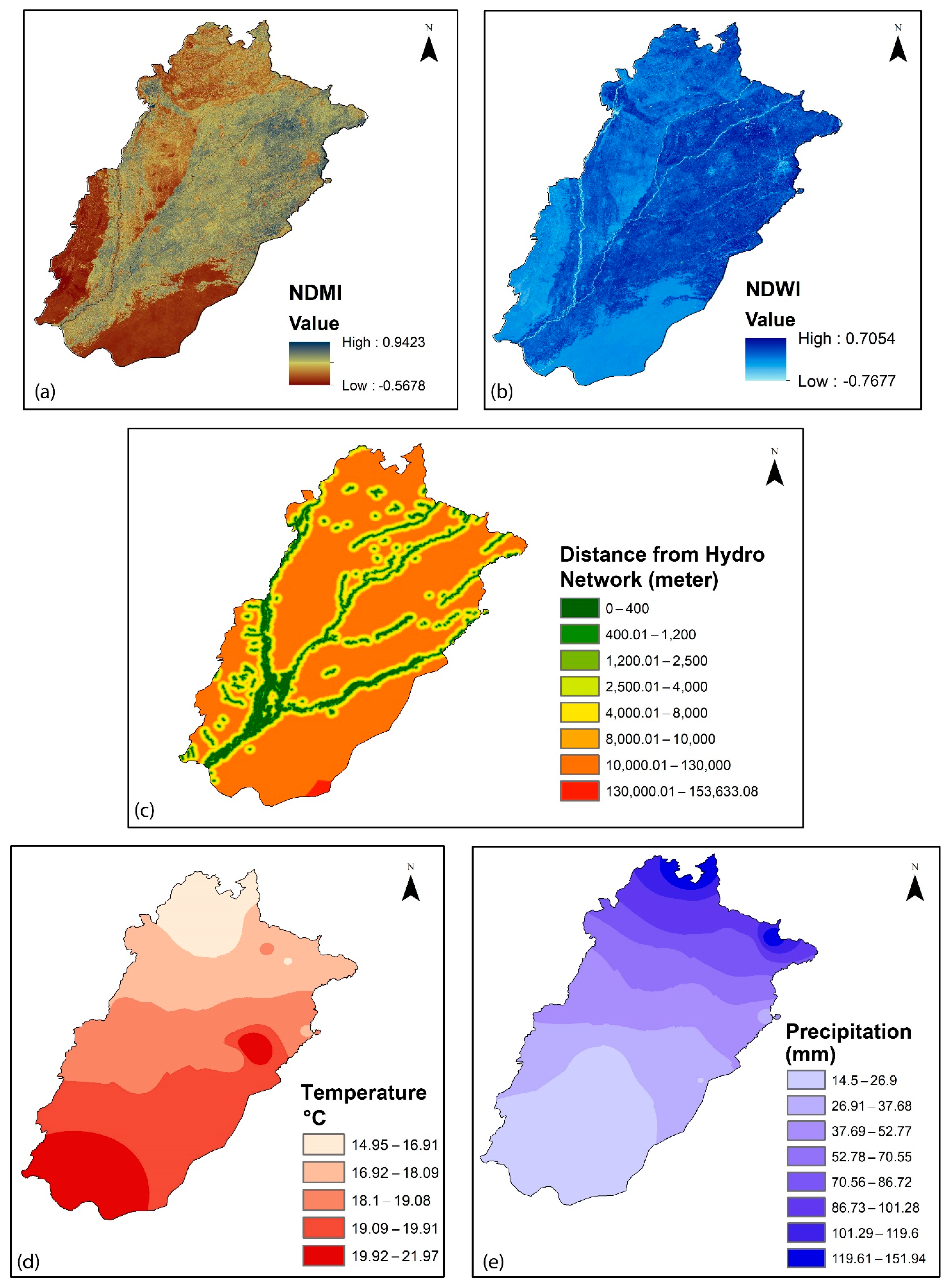
| Hydrometeorology (G1) | Normalized difference moisture index (NDMI) | j1 | NDMI evaluates the different contents of humidity from landscape elements, especially for soils, rocks, and vegetation. It is one of the important indicators adopted in EVA. The assessment of moisture content is essential to incorporate the health of vegetation perspective in the natural eco-environment of the region [81]. NDMI is calculated using the equation below [78]: NDMI = (NIR − SWIR1)/(NIR + SWIR1) (2) | Figure A1a |
| Normalized difference water index (NDWI) | j2 | NDWI is also called leaf area water-absent index, which implies the water content within vegetation. The index is derived from the reflectance properties of green vegetation, dry areas (lack of vegetation), and soils by using two near-IR bands. NDWI is calculated using Equation below. ([82]): NDWI = (G − NIR)/(G + NIR) (3) | Figure A1b | |
| Distance from hydrological network | j3 | Surface water is an important driver of natural eco-systems. According to experts, the areas that lack surface water are prone to desertification, forest fire, and landfill sites; therefore, areas farther from the hydrological network are more vulnerable and assigned more weightage in our EVA system. | Figure A1c | |
| Temperature | j4 | Temperature is a vital variable for EVA because it represents the climate conditions of the region. As the greenhouse gases in the atmosphere increase, the temperature will also increase. As a result, there is an increase in the melting of glaciers, which will first lead to extreme flooding followed by a scarcity of irrigation water [83,84]. This affects the vegetation growth of that area; therefore, the higher temperature implies higher vulnerability, and the lower temperature implies low vulnerability. | Figure A1d | |
| Precipitation | j5 | Precipitation is a vital variable for EVA because it represents the climate conditions of the region. Climate change is likely to involve changes in the amount and intensity of precipitation [15]. Changes in precipitation impact the hydrological, ecological, and biogeochemical processes, either directly or indirectly [85]; therefore, precipitation is incorporated in the EVA indicator system established in this study. Areas receiving huge rainfall annually are likely to be hit by extreme events such as floods and thus more vulnerable to eco-system health. | Figure A1e | |
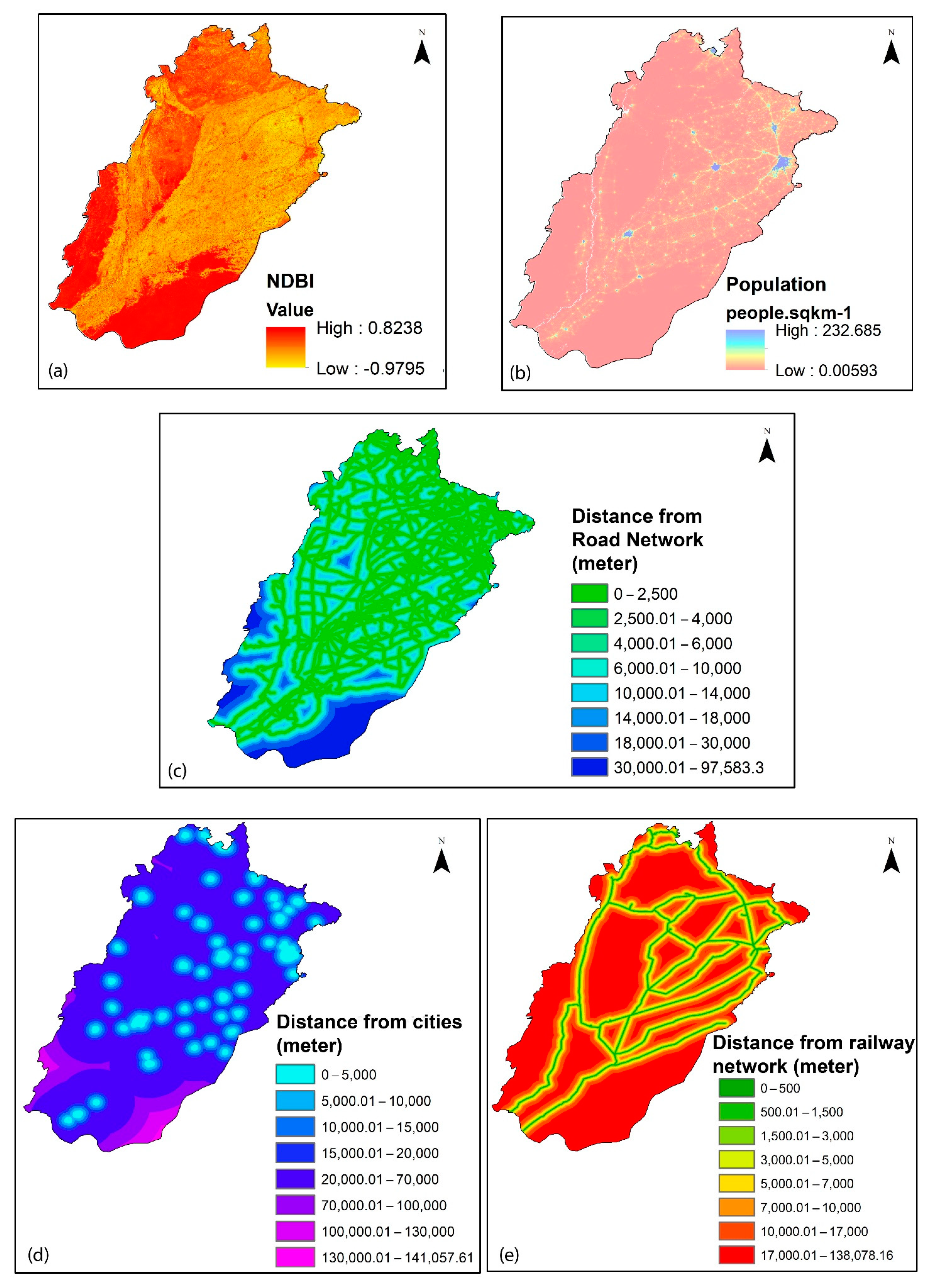
| Socioeconomics (G2) | Normalized difference built-up index (NDBI) | J6 | This variable is beneficial for the identification of human settlements and some elements of surrounding construction. It is a rapid and accurate method of mapping urban areas [86]. It can be calculated as: NDBI = MIR − NIR/MIR + NIR (4) Where NIR is the reflectance in the near-infrared band (Landsat OLI-TIRS band5 (0.845–0.885 μm)) and MIR represents the reflectance of the middle infrared band (OLI-TIRS band6 (1.560–1.651 μm)). | Figure A2a |
| Population | j7 | The population is an important variable for the quantification of vulnerable populations, in particular, vulnerable eco-systems. The high density of population reflects the pressure on natural resources and the intensity of economic activities [87]. | Figure A2b | |
| Distance from the road network | j8 | Similar to population, the distance to roads is an indicator in our EVA system to reflect the degree of human involvement. To avoid overestimating the influence of roads, only major roads such as highways, motorways are incorporated in the analysis. The regions nearest to the road network are assigned more weightage and areas farther away are less weightage. | Figure A2c | |
| Distance from cities | j9 | CPEC is primarily a corridor or connection between small and big cities for trade and economic growth; therefore, distance from the city center is indirect consideration of anthropogenic activity and urbanization. In general, cities stand for increased anthropogenic activity, industrial pollution, and fossil fuel exhaust from motor vehicles. Hence, the areas in close vicinity of cities are assigned more weightage in our EVA system. | Figure A2d | |
| Distance from the railway network | j10 | The construction of a new railway as well as upgrading existing railway lines are essential aspects of CPEC. The network of rail and road will boost trade and economic activities in the region. Thus, considering the distance from railway lines is vital for conducting EVA. Areas in closer proximity to railway lines will usually have higher vulnerability. | Figure A2e | |
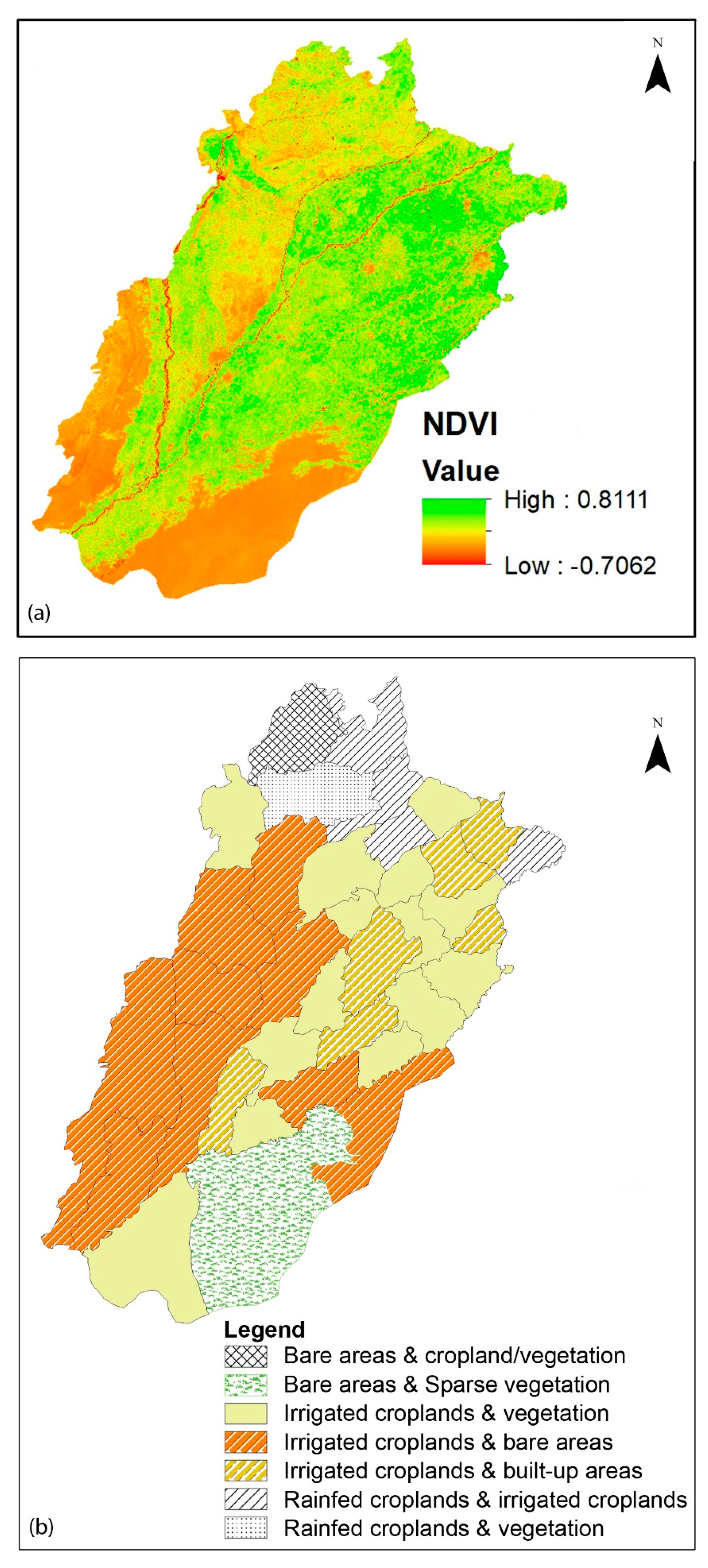
| Land resources (G3) | Normalized difference vegetation index (NDVI) | j11 | The normalized difference vegetation index is generated from the red and near-infrared (NIR) bands by the following simple expression: NDVI= (NIR-Red)/(NIR+Red). (5) It is a popular indicator used in EVA frameworks for incorporating the influence of vegetation and land use. High values of this index are obtained for areas covered by green vegetation. | Figure A3a |
| Land use land cover (LULC) | j12 | Land use/land cover is an important indicator of how human activities alter the natural land. The land surface characteristics have a direct relationship with surface energy balance, hydrological cycle, and eco-system services [88,89,90,91,92]. As revealed in literature, LULC is the essential indicator used extensively in EVA research [29]. Our EVA model also uses the dominant LULC layer as one of the inputs in the model. | Figure A3b | |
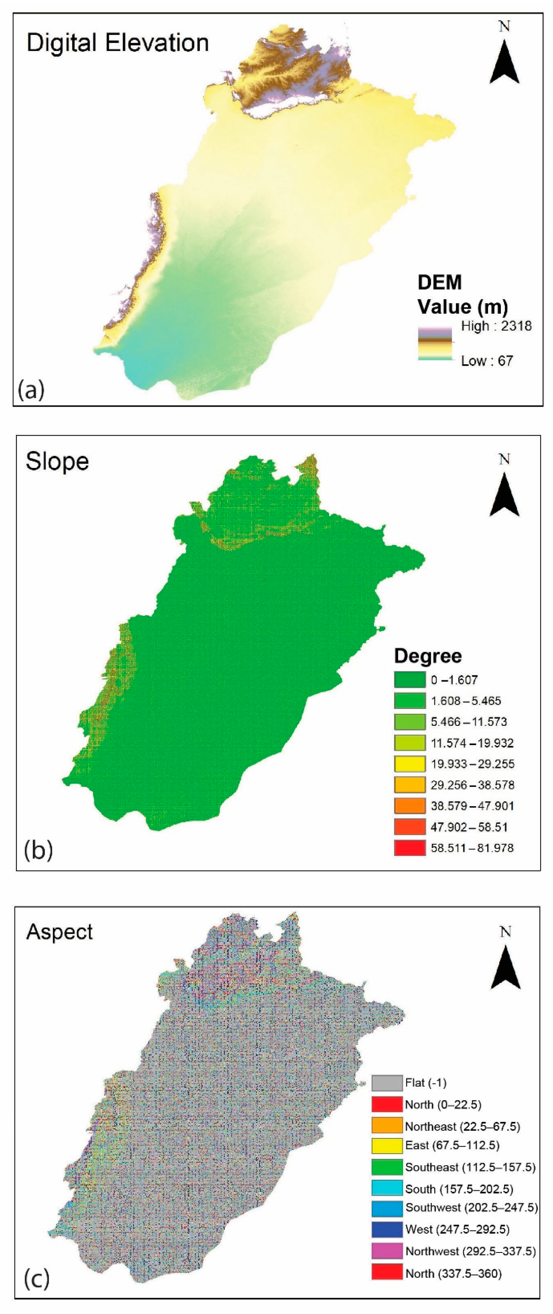
| Topography (G4) | Elevation | j13 | The elevation indicator in the EVA model represents the relief and terrain properties of the region. The elevation is a most important topographic characteristic that cannot be neglected in modeling-based research [93]. | Figure A4a |
| Slope | j14 | Slope direction and degree is a basic factor for eco-environmental vulnerability assessment because it impacts on climate conditions of the region. The slope influences hazards such as floods. | Figure A4b | |
| Aspect | j15 | The aspect is a popular indicator used in EVA research by various scientists. It plays a significant role in depicting surface characteristics in environmental research. | Figure A4c | |
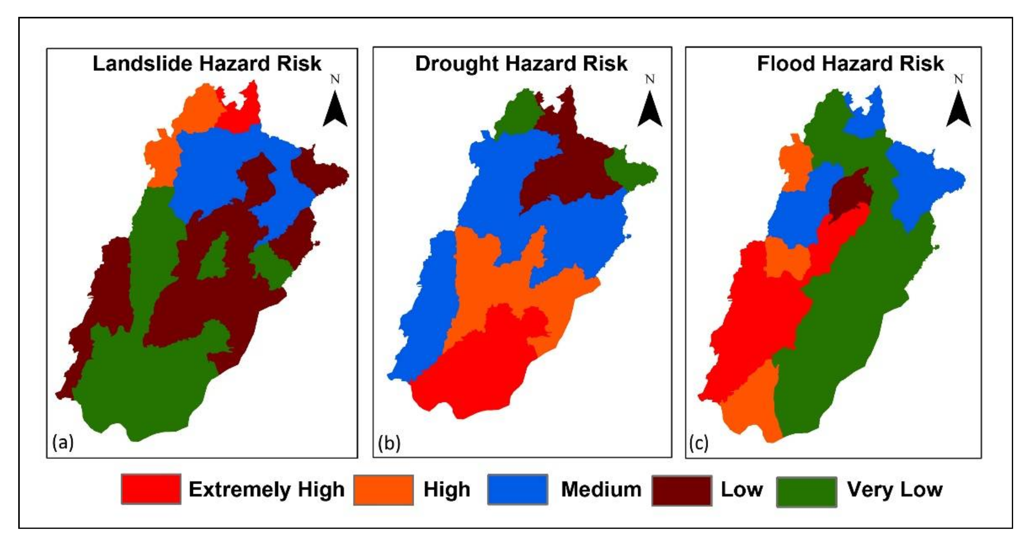
| Hazards (G5) | Drought hazard | j16 | Drought is a cycling recurring natural event that affects environmental, economic, and social conditions [94]. It has been widely incorporated in vulnerability modeling research. In our EVA framework, more weightage is assigned to an area where drought hazard is “very high”. | Figure A5a |
| Flood hazard | j17 | Flood is the most prevalent and devastating natural disaster among all-natural disasters that adversely impact human health and natural and artificial environments [95,96]. It has been widely incorporated in vulnerability modeling research. In our EVA framework, more weightage is assigned to the area where flood hazard is “very high”. | Figure A5b | |
| Landslide hazard | j18 | Landslides are the downslope movements of debris, rocks, or earth material under the influence of the force of gravity. The areas where landslides occur frequently are highly vulnerable in terms of deaths, infrastructure damages, and environmental losses [97]; therefore, it is a widely used indicator in vulnerability modeling research in literature. In our EVA framework, more weightage is assigned to the area where landslide hazard is “very high”. | Figure A5c | |
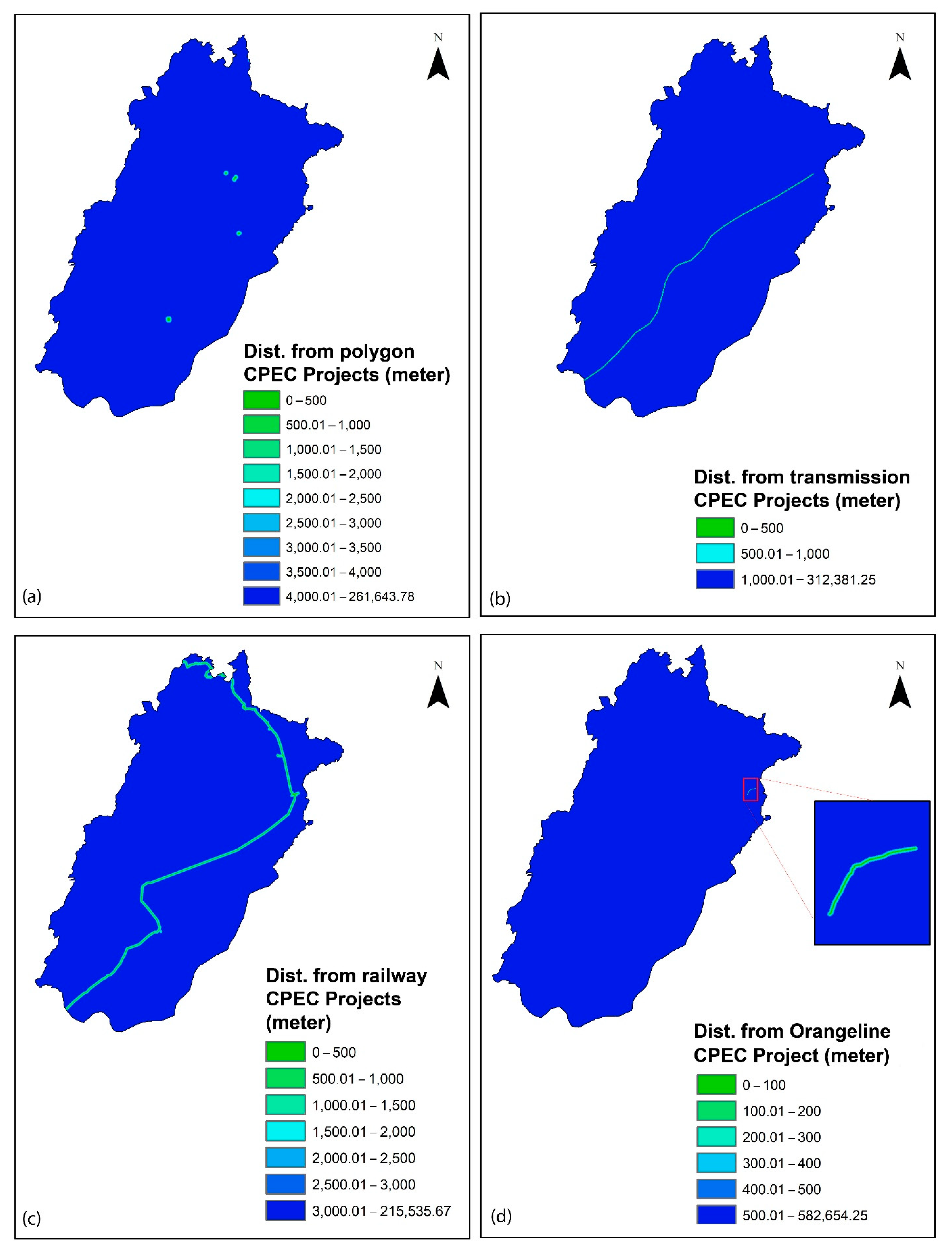
| CPEC projects (G6) | Distance from polygon CPEC projects | j19 | The group of CPEC projects represents a truly multidisciplinary system that signifies environmental concerns and economic growth. A total of eight projects are included in the study. Five out of eight can be represented as polygons. These projects include coal power plants, special economic zones, etc. Buffer distance is used to assign more weightage to the area very close to the project. | Figure A6a |
| Distance from linear CPEC projects | j20–22 | Three out of eight projects can be represented as line features in the GIS environment, such as transmission line, railway, and orange line in-city mass-transit project. Their influence in the EVA model is different from those that can be represented as polygons; therefore, the polygon and linear projects are separated in our EVA model. | Figure A6b–d |
| First Grade (EVA) | Second Grade (G) | No. | Weights-G | Third Grade (ji) | No. | Weights-i |
|---|---|---|---|---|---|---|
| EVA | Hydrometeorology | G1 | 0.138 | Normalized difference moisture index (NDMI) | j1 | 0.068 |
| Normalized difference water index (NDWI) | j2 | 0.052 | ||||
| Distance from hydrological network | j3 | 0.454 | ||||
| Temperature | j4 | 0.245 | ||||
| Precipitation | j5 | 0.181 | ||||
| Socio-economics | G2 | 0.197 | Normalized difference built-up index (NDBI) | j6 | 0.063 | |
| Population | j7 | 0.591 | ||||
| Distance from Road Network | j8 | 0.097 | ||||
| Distance from Major Cities | j9 | 0.113 | ||||
| Distance from Railway Network | j10 | 0.136 | ||||
| Land Resources | G3 | 0.09 | Normalized difference vegetation index (NDVI) | j11 | 0.643 | |
| Land use and land cover | j12 | 0.357 | ||||
| Topography | G4 | 0.176 | Elevation | j13 | 0.597 | |
| Slope | j14 | 0.182 | ||||
| Aspect | j15 | 0.091 | ||||
| Hazards | G5 | 0.137 | Drought hazard | j16 | 0.236 | |
| Flood hazard | j17 | 0.451 | ||||
| Landslide hazard | j18 | 0.313 | ||||
| CPEC Projects | G6 | 0.262 | Dist. from Polygon CPEC Proj | j19 | 0.347 | |
| Dist. from Transmission CPEC Proj | j20 | 0.193 | ||||
| Dist. from Railway CPEC Proj | j21 | 0.284 | ||||
| Dist. from Orangeline CPEC Proj | j22 | 0.176 |
Publisher’s Note: MDPI stays neutral with regard to jurisdictional claims in published maps and institutional affiliations. |
© 2021 by the authors. Licensee MDPI, Basel, Switzerland. This article is an open access article distributed under the terms and conditions of the Creative Commons Attribution (CC BY) license (https://creativecommons.org/licenses/by/4.0/).
Share and Cite
Kamran, M.; Bian, J.; Li, A.; Lei, G.; Nan, X.; Jin, Y. Investigating Eco-Environmental Vulnerability for China–Pakistan Economic Corridor Key Sector Punjab Using Multi-Sources Geo-Information. ISPRS Int. J. Geo-Inf. 2021, 10, 625. https://0-doi-org.brum.beds.ac.uk/10.3390/ijgi10090625
Kamran M, Bian J, Li A, Lei G, Nan X, Jin Y. Investigating Eco-Environmental Vulnerability for China–Pakistan Economic Corridor Key Sector Punjab Using Multi-Sources Geo-Information. ISPRS International Journal of Geo-Information. 2021; 10(9):625. https://0-doi-org.brum.beds.ac.uk/10.3390/ijgi10090625
Chicago/Turabian StyleKamran, Muhammad, Jinhu Bian, Ainong Li, Guangbin Lei, Xi Nan, and Yuan Jin. 2021. "Investigating Eco-Environmental Vulnerability for China–Pakistan Economic Corridor Key Sector Punjab Using Multi-Sources Geo-Information" ISPRS International Journal of Geo-Information 10, no. 9: 625. https://0-doi-org.brum.beds.ac.uk/10.3390/ijgi10090625