1. Introduction
Earthquakes have significantly impacted economic and social losses in urban areas because they have brought extensive damage to buildings and infrastructures. Building damage is the most critical factor of seismic losses because buildings are the predominant facility in the built environment, and buildings are vulnerable to earthquake damage [
1]. Building damage estimations for earthquake scenarios have been recognized as essential information for planning disaster reduction measures.
Population growth, urban expansion, and building density have developed significantly in Ulaanbaatar city (UB), the capital of Mongolia. UB’s current population reaches approximately 1.5 million, which corresponds to about half of Mongolia’s population. Mongolia has suffered large earthquakes triggered by active faults [
2,
3,
4]. However, no significant earthquake has been reported in UB due to low population density, nomadic lifestyle, and poor earthquake observation stations before starting the instrumental period in 1957. Recent earthquake observations in Mongolia revealed the seismic activities in and around UB have been limited to moderate earthquakes with a magnitude less than 4.5 [
5]. During the last century, the maximum seismic intensity with the MSK scale at UB was VI [
5].
Although large earthquakes have not yet been recorded in the UB area, several active faults exist around the UB area, such as Emeelt, Hustai, Sharhai, and Gunjiin faults [
6]. A fault was recently found just beneath the UB metropolitan area [
7]. These active faults have been expected to be capable of causing earthquakes with a magnitude of 7 or larger. However, UB has not fully developed the geophysical and building inventory database required for strong motion prediction and building damage estimation in earthquake scenarios. Although the Japan International Cooperation Agency (JICA) performed a simple earthquake damage estimation in UB [
8], detailed soil conditions and building vulnerabilities in UB were not considered in the previous estimation.
Building damage estimation methodologies can be divided into estimations based on fragility and vulnerability functions [
9]. The former method estimates probabilities of damage level for a building using the fragility function that represents the relationship between seismic excitation and damage probability. Seismic excitation includes ground motion intensity or building response spectrum with damage probability for each damage state such as collapse, severe damage, moderate damage, and slight damage developed for various building structural types. In typical approaches of the method, such as HAZUS [
10,
11,
12], building damage probabilities were estimated from building responses derived by the spectral capacity method using demand curves of ground motions and capacity curves of buildings. In alternative approaches, building damage was estimated by empirical fragility curves developed from ground motion intensities and building damage statistics obtained in past damaging earthquakes [
13,
14]. The fragility function-based approach can estimate the number of damaged buildings expected from predicted ground motion intensities.
The latter method estimates building loss based on vulnerability functions developed for each structural type [
15,
16]. Vulnerability functions represent the relationships between ground motion intensity and repair cost normalized by the replacement or construction cost. The normalized repair cost in percentile is expressed as the mean damage ratio (MDR) with variance in the vulnerability functions. Thus, the economic losses of buildings in earthquake scenarios can be directly quantified by the vulnerability functions. Recently vulnerability functions for various building structural types have been developed to globally assess the seismic risk of buildings [
17,
18,
19]. If a database of construction costs for buildings in a target area is obtained, direct building monetary losses can be evaluated for an earthquake scenario using the vulnerability functions [
20].
The last factor of the damage assessment is the building inventory database, which represents the census data on the housing [
21]. Regional and national level seismic evaluation requires low-resolution distribution of buildings on the district or regional scale. A High-resolution database is essential for detailed damage assessment, but it is time-consuming and costly [
22]. This study aims to develop a building inventory database in UB, including the construction cost for each building in considering structural types, building heights, heating types, and other building characteristics in order to economically assess the buildings’ vulnerabilities for a scenario earthquake.
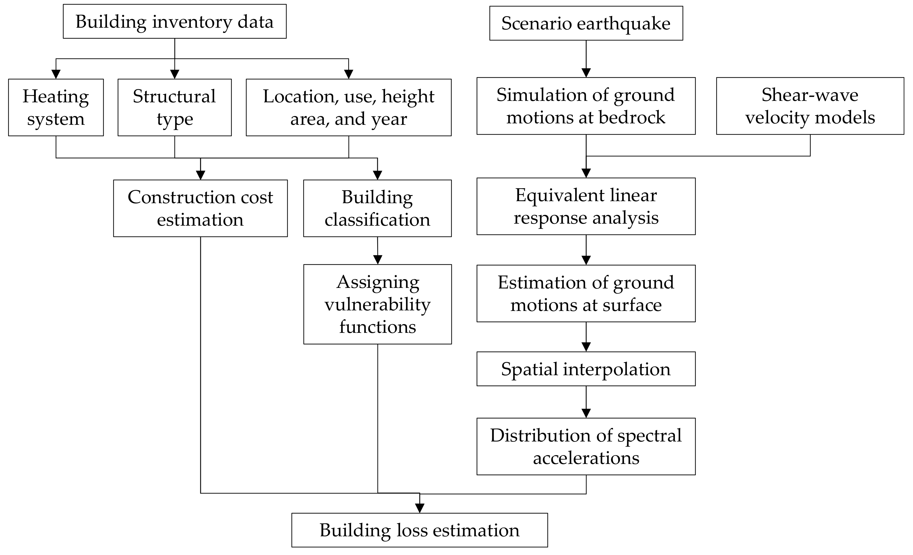
Figure 1 shows the flowchart of the analysis in this study. Although existing building inventory data are available in UB, structural types and construction years necessary for construction cost estimation and assignment of vulnerability functions are not fully registered in some buildings. We estimate the structural types, construction years, and heating types by criteria developed from the building characteristics in the inventory data. The construction cost for each building in UB is estimated by applying the procedure adopted in the Ministry of construction and urban development of Mongolia [
23]. Strong motion simulation is performed for a scenario earthquake by the Emeelt fault using the stochastic Green’s function method [
24,
25,
26] and the equivalent linear ground response analysis [
27] based on the shear-wave velocity structures [
28]. Direct building losses in UB are estimated by aggregating the repair costs of the damaged buildings estimated from the predicted ground motion intensities and the global vulnerability functions [
17,
19]. Economic loss in UB expected from the earthquake scenario is discussed in terms of Mongolia’s gross domestic product (GDP).
2. Development of Building Inventory Data
2.1. Existing Building Inventory Data
The Geographical Information System (GIS)-based building inventory database in UB was firstly established by the Korea International Cooperation Agency (KOICA) in 2010. The database has been updated by the UB city office and was used in the seismic risk assessment by JICA [
8]. The inventory data includes more than 32,000 buildings with location information, a number of stories, main structural type, building area, and construction year, as shown in
Table 1.
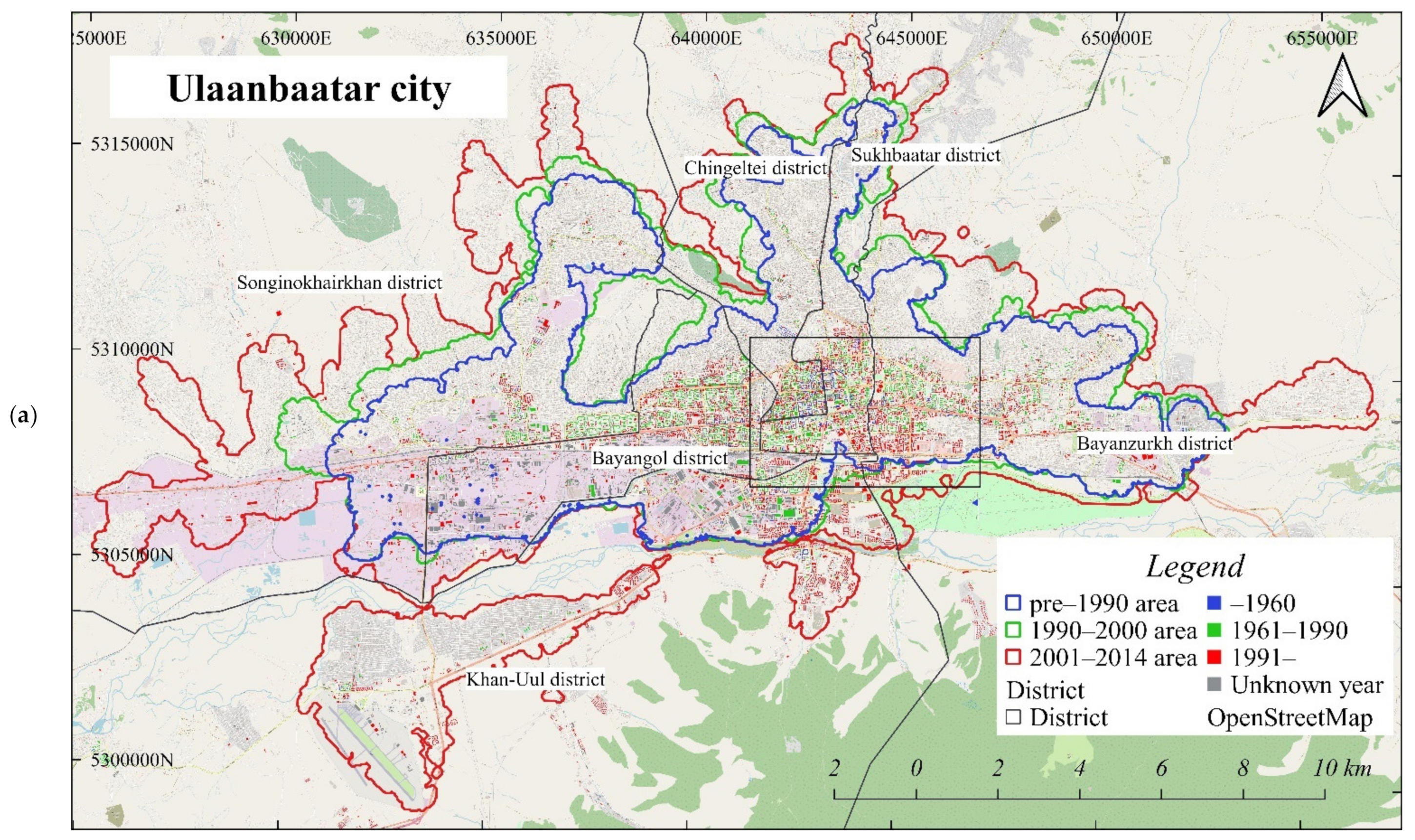
Figure 2a,b shows the distribution of the construction year and building heights of the existing building inventory in UB, respectively.
Figure 2a also illustrates the areas of the urban sprawl in UB [
29].
Figure 2b also illustrates urban land use such as residential, office, and industrial areas [
30]. Ger is a traditional Mongolian dwelling that consists of a round felt tent covered with durable, waterproof, white canvas. Since many ger houses exist outside the land use areas, we added the ger areas in
Figure 2b by manually delineating the boundaries from the current building distribution. Although ger-type houses have been built mainly in the ger areas around mountainous areas, ger houses have not been registered in the inventory data. Therefore, ger houses are not considered in this study. Low-rise (1–3 stories) buildings typically dominate in the ger areas, and mid-rise and high-rise buildings are highly concentrated in the central office and residential areas.
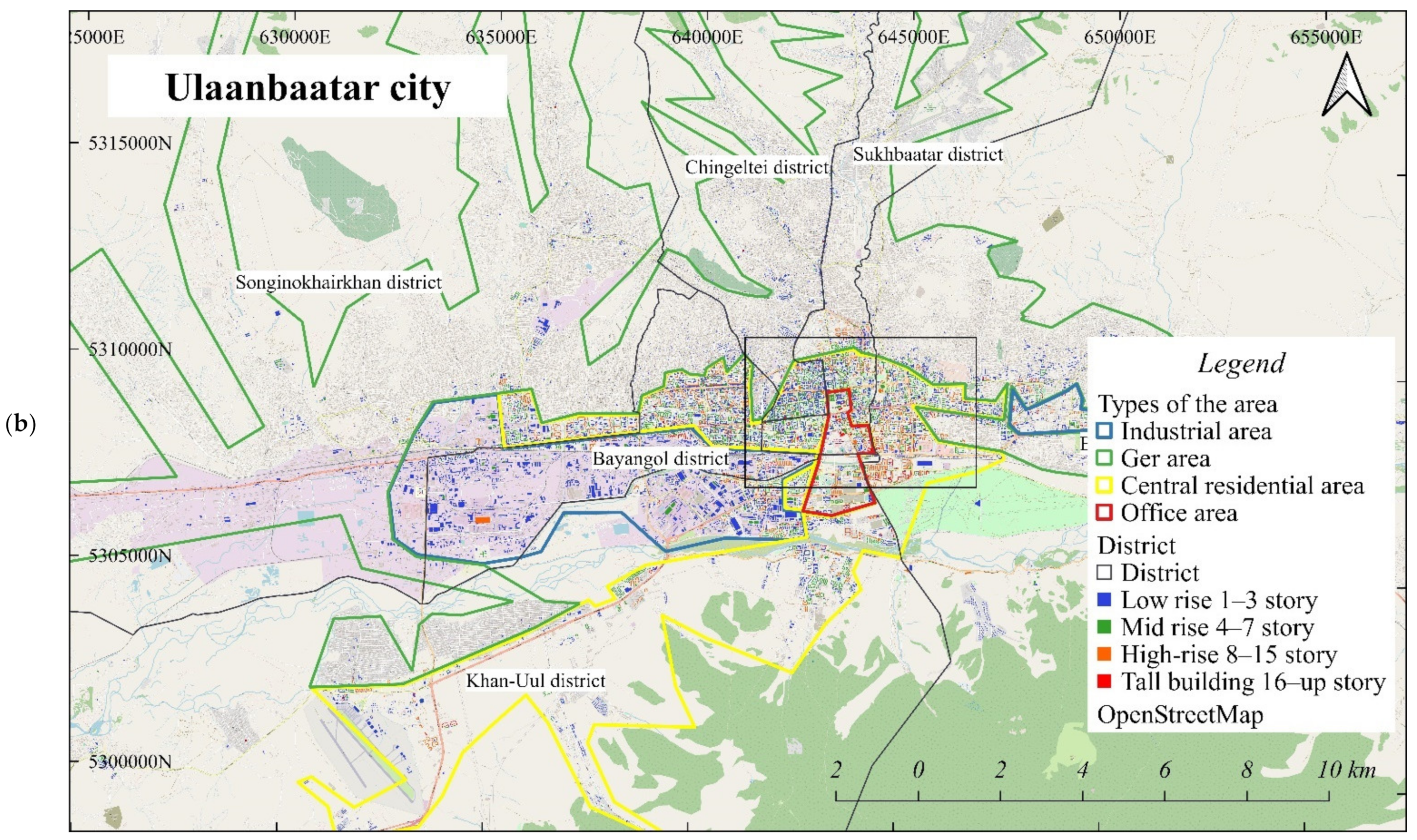
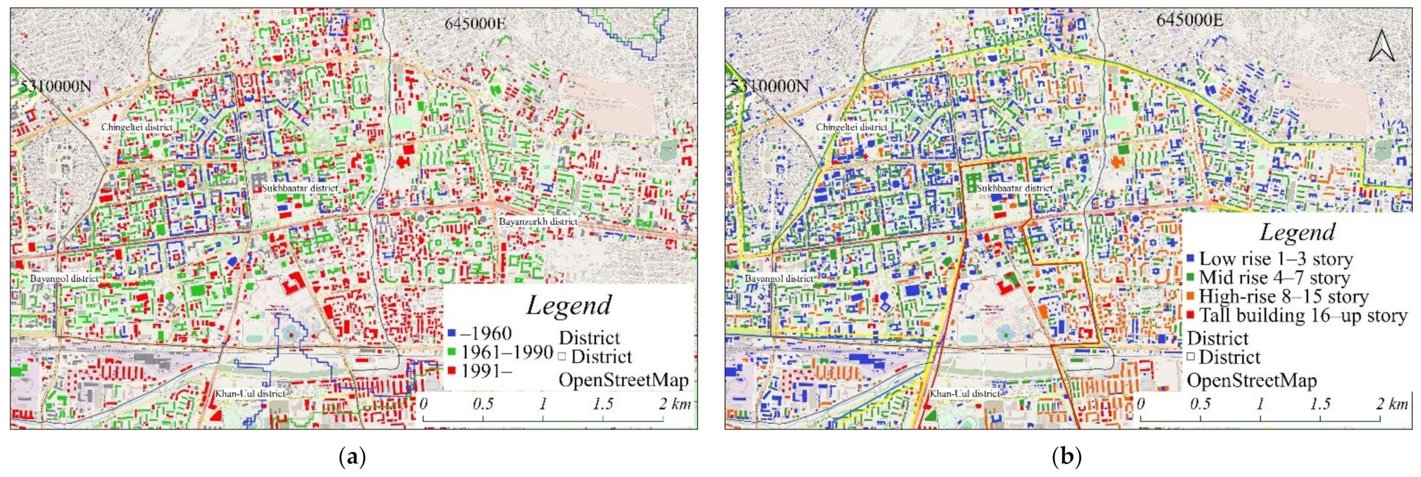
Figure 3a,b represents the close-ups of the central part of UB as shown by the rectangle in
Figure 2a,b, respectively. Building information was assigned for an individual building in the GIS inventory data.
Table 2 shows the number of buildings in the inventory data according to structural types and building heights. In total, 32,500 buildings are included in the inventory data. Approximately 85% of the buildings are low-rise buildings. The number of high-rise buildings higher than 16 stories is about 300. The structural types are masonry, timber, reinforced concrete (RC) frame, RC frame with a masonry wall, RC frame with a shear wall, precast, and steel structures. However, the structural types for more than 50% of the buildings are not registered (unknown). Besides, masonry and timber buildings seem erroneous. For example, many masonries and timber buildings are higher than four stories despite most of those building types being low-rise. In the first recording of the inventory, misclassifications would be generated. If some part of the roof and/or exterior walls in nonstructural elements of the building were wood or brick, the main bearing structures were incorrectly listed as wooden or brick.
Table 3 shows the number of buildings with construction years. Similar to the structural types, construction years for more than 60% of the buildings are unknown. Most of the unknown buildings can be classified as buildings constructed before 2010 because building officials rarely registered the older buildings. In contrast, most of the newly constructed buildings after 2010 have been almost fully registered in the inventory.
The heating system of each building is essential information for estimating construction costs in UB described later. However, such information is not included in the inventory. The existing building inventory data issues for estimating construction costs can be summarized below. First, structural types of unknown, masonry, and timber buildings need to be estimated. Second, the construction years for unknown buildings need to be estimated, and last, the heating system of each building needs to be estimated.
2.2. Procedure for Construction Cost Estimation
The building costs of the buildings in UB are estimated using the Mongolian construction code [
23]. According to the procedure, this code estimates the budgeted cost of a building, which is provided to investors, customers, and contractors with the same conditions and information to determine the cost of construction. The construction cost includes the direct cost of the entire construction, including materials, supplies, labor, tools, equipment, machines, and transportation. It excludes the cost of land acquisition for the construction of the facility, the cost of relocating the utilities, and the cost of the plant’s construction technology equipment, as well as the cost of the land and sales. The Ministry of construction and urban development in Mongolia published the latest code in 2016, which is suitable for this research data. The total cost depends on the individual building area and other coefficients of local conditions, such as the building heating system, location, structural type, and inflation rate, as shown in Equation (1).
cost(MNT/m2)—building unit cost per floor area for building type in MNT (Mongolian Tugriks as of 2016, 1.0 USD = approximately 1550 MNT).
area(m2)—building floor area in square meters.
Knature(GIS)—coefficient for natural influence by the soil and weather., I: 1, II: 1.05, III: 1.10, IV: 1.18, V: 1.25 [
23], 1.0 in UB area.
Kdistance(GIS)—coefficient for transportation fee [
23], 1.0 in UB area.
Kheating—coefficient for heating system in each building. Buildings in the central district are connected to central heating system 1.0, individual heating type 0.95, and simple heating stove 0.75.
Keconomy—coefficient for the economic condition at each year, 1.0 as of 2016.
Kreduction—coefficient for reducing area considered with outer wall space, normally 1.0.
Since the target area of this research is the central districts of UB city, all the buildings are located within 50 km from UB, and the coefficients Kdistance, Knature, Keconomy, and Kreduction are given at 1.0, respectively. Since Mongolia is located in a cold region, the heating system of a building is one of the critical parameters in evaluating construction costs. The building unit cost per floor area is determined according to the structural type introduced later. This means that the structural type and heating system need to be determined for each building in order to estimate the construction cost. Besides, the construction year also needs to be estimated to assign the design level of vulnerability functions.
Despite the lack of building information in the existing inventory data, the building distribution in UB suggests that typical building types can be characterized by other building information such as the location, building use, building area, and the number of stories. This study estimates structural types and construction years for the unknown buildings by criteria developed from the building characteristics in the existing building inventory. The details of each estimation are introduced in the following sections.
2.3. Estimation of Heating System
Since it is difficult to find information about the heating system coverage map, the coefficient
Kheating is estimated from the existing GIS data by defining the heating-system-connected area of UB. In general, residential apartments are connected to the central heating system in the central regions of UB. Most households located around mountain areas such as the ger areas are not connected to the central city system. Simple heating stoves and individual heating types are typically used for small houses and industrial buildings, respectively.
Table 4 shows the criteria for the estimation of a heating type for each building. The heating type is determined by the building location, structural type, and building area. Small and low-rise buildings in the ger area are classified as having a simple heating stove. Two-story buildings whose building use and structural type are both unknown, and two-story small masonry or timber buildings, are also assigned to the simple heating stove. Buildings in the ger area whose building use or structural type is already given in the inventory are classified to the individual heating type. Outside the ger area, 1–2-story small precast or steel buildings are also classified as the individual heating type. Other buildings outside ger areas are classified as the central heating system. The numbers of the classified buildings are shown in the last column of
Table 4. A smaller coefficient is given to the buildings with a simple heating stove, and a higher coefficient is given to the buildings with the central heating system, as shown in Equation (1).
2.4. Estimation of Structural Type and Construction Year
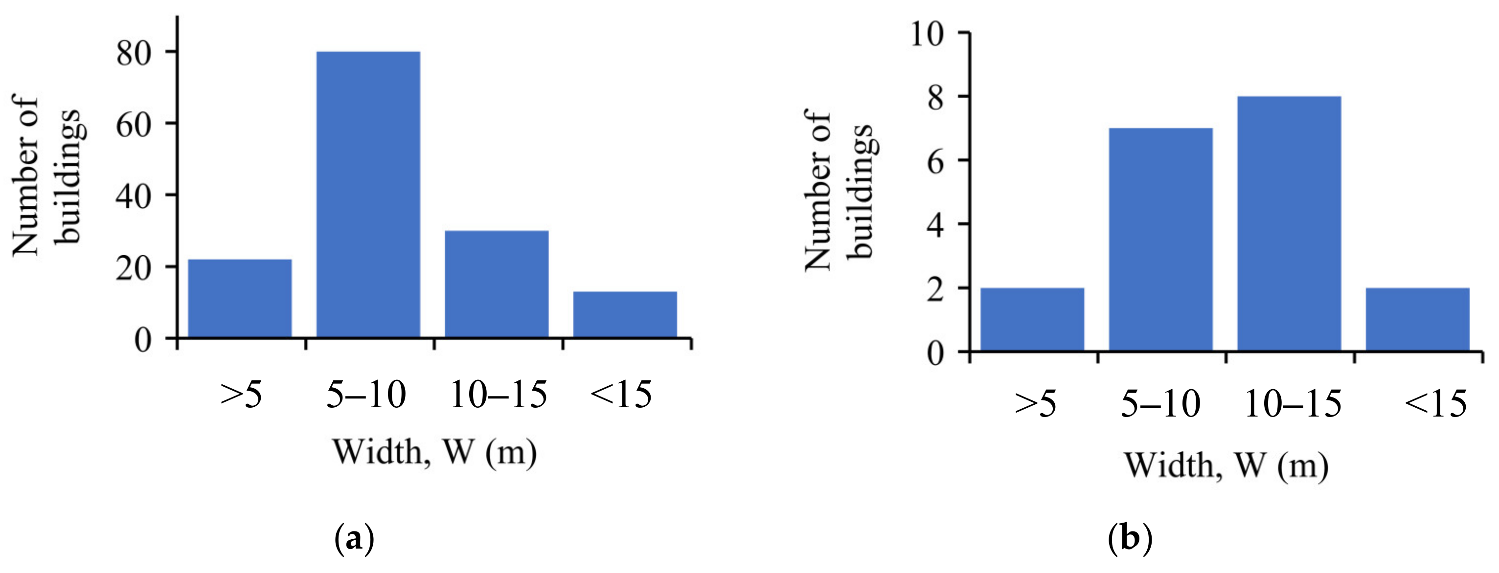
The building structural type is important information to estimate the construction cost and to assign vulnerability functions for seismic loss estimation. The location, number of stories, building area, and shape of the building classify the structural types of the unknown buildings. The building area, width, and length of buildings are considered in the classification because the building shape would be a key parameter to assign the structural type. The width and length are approximated from the area and perimeter of a building polygon.
Figure 4 shows a histogram of building width in the existing known data for (a) 1-story masonry buildings and (b) 1-story RC with masonry wall buildings in the office and central residential areas, respectively. Based on this chart, the majority of the width for the masonry buildings is less than 10 m, and that for the RC with masonry wall is more than 10 m. We classified the 1-story unknown buildings to masonry and RC with masonry walls by using the threshold value of 10 m in building width.
As shown in
Figure 4, the threshold values to classify the structural types for unknown buildings are determined by the distribution of the histograms for building shapes such as area, length, and width in the registered buildings in the existing inventory data. This means that the buildings classified by thresholding using the criteria constitute the majority of the registered buildings. If the significant difference between the shape information between the structural types was not observed in histograms, the shape information was excluded from the classification.
Table 5 shows the criteria for estimating structural types for unclassified buildings. The unknown buildings are classified as masonry, timber, precast, steel, and RC with masonry wall structures. The small and low-rise buildings are classified into masonry or timber structures. On the contrary, larger and higher buildings are classified as precast, steel, or RC with masonry wall structures. If the buildings are located in the industrial area, the buildings are classified as precast or steel frames. The majority of structural types in the known buildings are masonry for low-rise buildings, RC with a masonry wall for mid-rise buildings, and RC for high-rise buildings. Therefore, the unknown buildings that satisfy the specific criteria in
Table 5 are classified as timber, precast, and steel structures. Other unknown buildings were classified as masonry, RC with a masonry wall, and RC structures. The numbers of the classified buildings are shown in the last column of
Table 5. As described before, some misclassifications are also found in the classified buildings. According to the Mongolian seismic code, the load-bearing structure of a building with more than five floors cannot be made of bricks, but there is an error in these data as there are tall brick buildings. Therefore, tall masonry buildings are re-classified to RC with masonry or RC with shear wall depending on the number of floors. The high-rise timber and RC buildings are re-classified to RC with masonry walls or RC with a shear wall, and large timber buildings in industrial areas are steel structures. We have to pay attention to the fact that it is still difficult to accurately classify all the structural types by the thresholding approach because there are overlapping parts in the histograms, as shown in
Figure 4.
The estimated structural types are validated by comparing them with the field photographs.
Figure 5 compares the structural types estimated by the proposed method and the pictures of typical buildings in the StreetView of Google Map [
31]. The upper three buildings in
Figure 5 were classified as unknown in the existing inventory data and are classified as masonry, precast, and RC with a masonry wall, respectively. Whereas the original structural type of the building shown at the bottom of
Figure 5 was timber, the type is obviously erroneous when comparing it to the field photo. The building is re-classified to RC by the proposed criteria. Whereas it is difficult to identify the actual structural type from the field photo, the results show that the estimated structural types seem reasonable to the conditions of the actual buildings. The collection of actual structural-type information for many buildings would require much labor and time. Field investigations would still be needed in order to justify our estimations comprehensively.
Since it is difficult to accurately estimate the construction year from the existing inventory data alone for an individual building, the urban sprawl map shown in
Figure 2a is used in the estimation.
Table 6 shows the criteria for the estimation of the construction year. As previously described, most of the unknown buildings are assumed to be constructed before 2010. The parameters used in the criteria are the location, number of stories, building area, and structural type. Most timber and precast buildings were constructed before and during the period of the influence of the Soviet Union. If the structural type of the target building is timber or precast, the construction year is classified as an older building constructed before 1990. Large steel or masonry buildings are also classified as older buildings, constructed before 1990. If the number of stories is higher than 12, the construction is classified as a newer building constructed after 2001. Other buildings are classified as structures built from 1991 to 2000. The numbers of classified buildings are shown in the last column of
Table 6.
2.5. Construction Cost Estimation
The construction costs for all the buildings in UB are estimated from Equation (1).
Table 7 shows the construction cost per unit in USD for each building use and structural type. A higher cost is required for house and office buildings with RC frame structures. On the other hand, a lower cost is required for storehouses or cellars with masonry or steel structures. By using the cost per unit, structural type, building use, and floor area, the total amount of construction cost is estimated for each building.
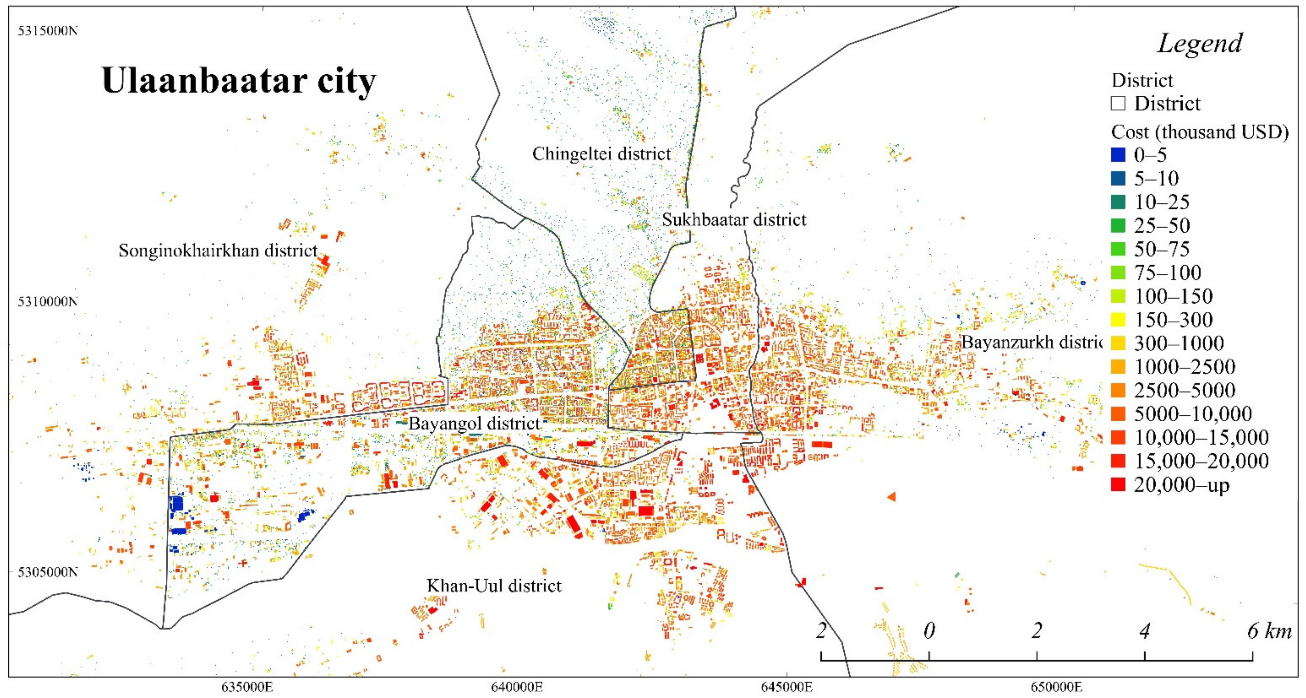
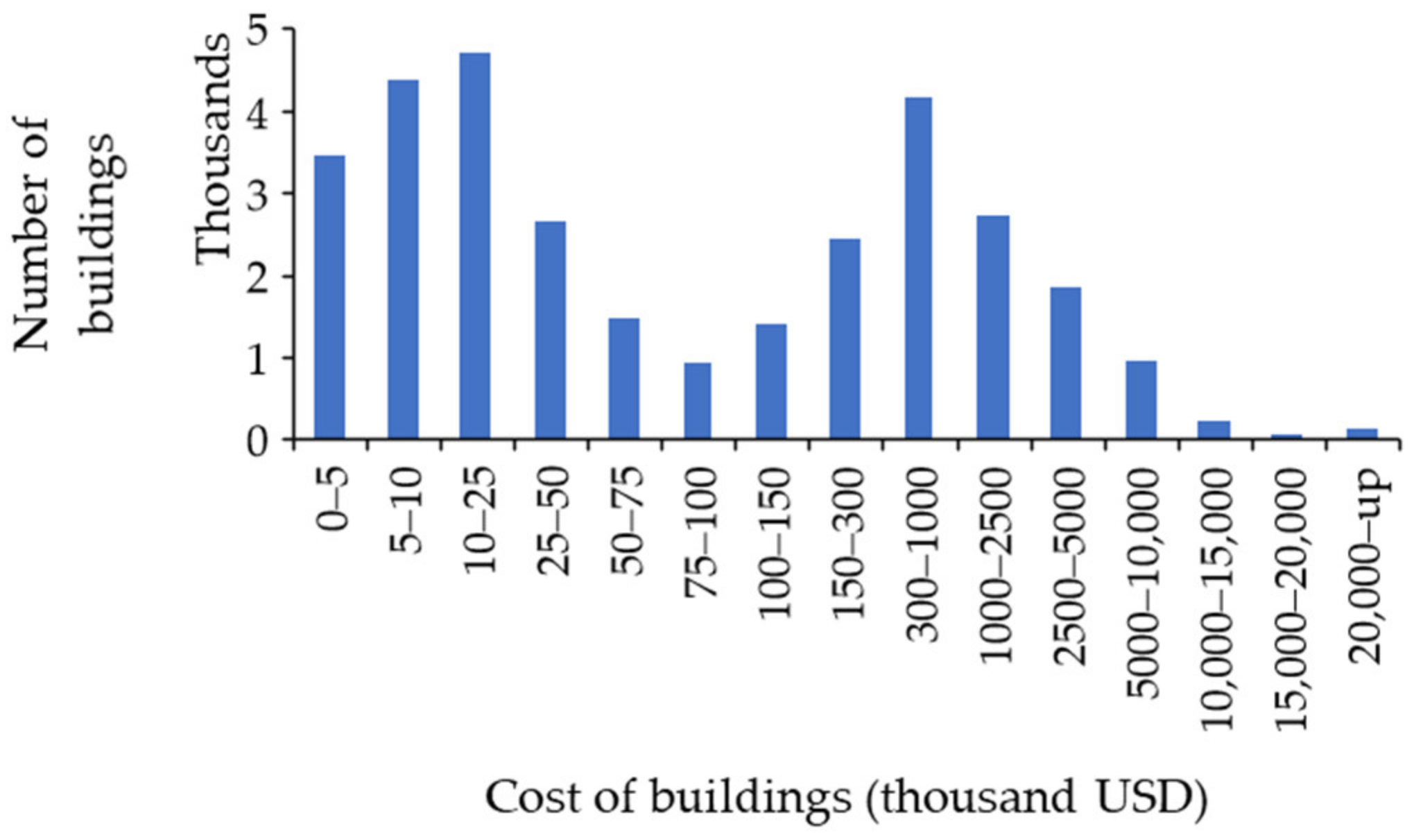
Figure 6 shows the estimated construction cost distribution of UB.
Figure 7 shows the histogram of the number of buildings according to the construction costs. Around 13,000 buildings’ cost is lower than 25,000 USD, which corresponds to small buildings located in the ger area. Approximately 4000 buildings cost from 300,000 to 1 million USD, and most of them are located in the central residential area. The buildings whose construction cost is higher than 500 million USD correspond to the high-rise buildings located in the city’s central office area. Whereas the estimation is based on the currency as of 2016, we can estimate the current prices considering the change in currency for a year of interest.
The statistic department of the Ulaanbaatar city office has published the total amount of property in several districts from 2006 [
32]. The city authorities have developed statistical data with each year based on the procurement report every year. Since the number of buildings constructed after 2010 in the inventory data would be more reliable than those of older buildings, our estimation is compared with the statistics since 2010.
Figure 8 compares the total amount of costs in six districts (SHD: Songinokhairkhan district, HUD: Khan-Uul district, BZD-Bayanzurkh district, BGD: Bayangol district, SBD: Sukhbaatar district, and CHD: Chingeltei district) with the statistics for each year after 2010. Our estimations in SHD and SBD show good agreement with the statistical data. However, the estimations in BZD and CHD are remarkably smaller than the statistics. One of the underestimations might be that BZD and CHD include many ger areas where a number of unregistered buildings have been constructed. Since our estimation did not consider ger houses, our estimation would be significantly smaller than the statistics.
2.6. Assignment of Vulnerability Functions
In this study, the global vulnerability functions developed in the GAR-13 [
17,
18,
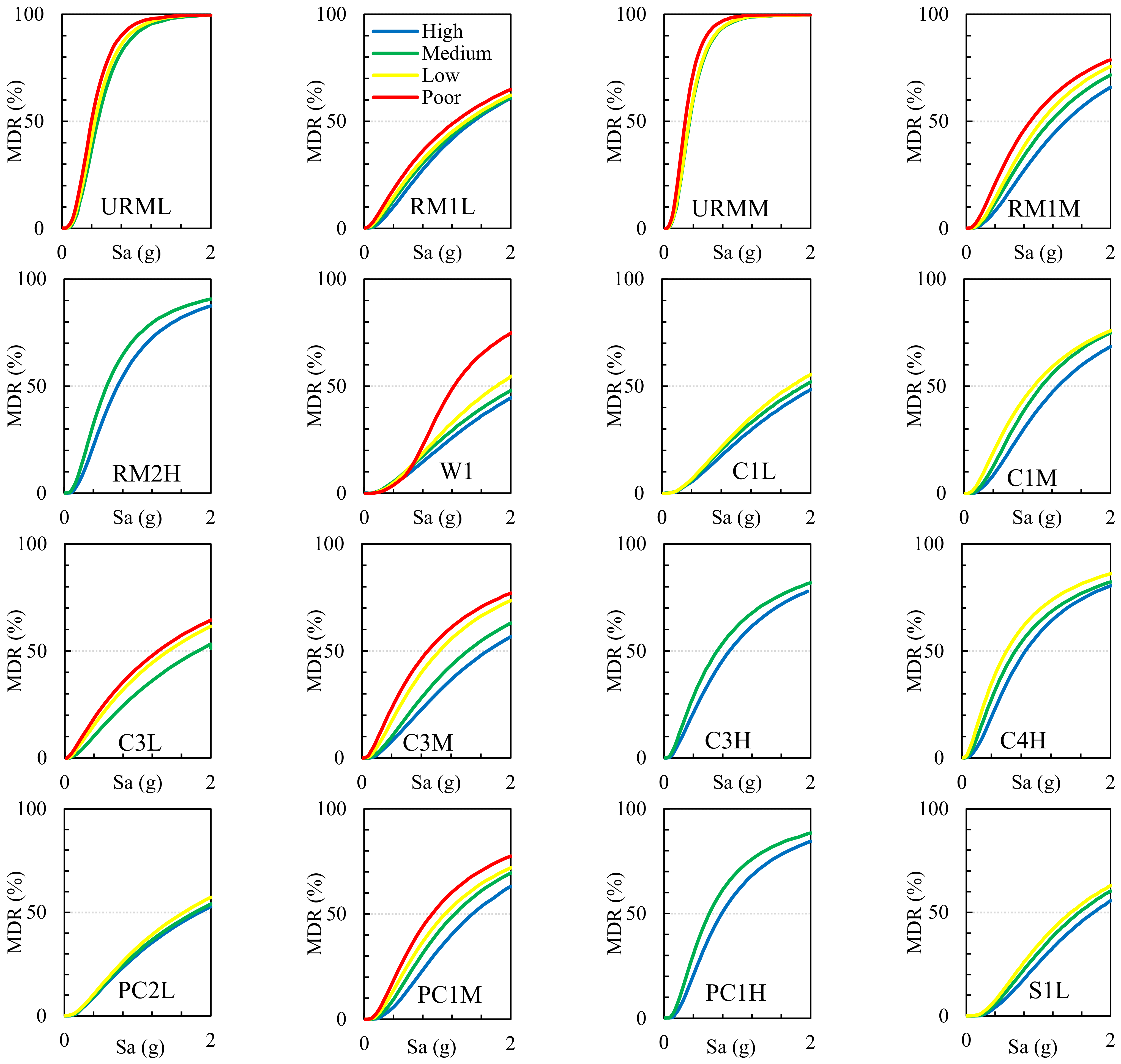
19] are used to estimate building losses by a scenario earthquake. The seismic vulnerability functions of the GAR-13 represent the relationship between spectral acceleration for the typical period of a building class and expected repair cost in percentage (mean damage ratio: MDR). The vulnerability functions were developed for 47 building classes considering structural types and building heights, and four design levels (High, Medium, Low, and Poor) in the GAR-13.
We assign each building in the updated inventory data to the classes of GAR-13 based on the criteria shown in
Table 8. The building classes are classified considering the structural type and the number of stories. The design levels are classified considering the building location, building use, and construction year. Since many non-engineered masonry houses exist in ger areas, poor design level is given to the buildings in the ger areas. The higher design level is assigned to public buildings such as government buildings, city offices, schools, and hospitals. The building area and construction year are considered in classifying the design levels of masonry, timber, and RC with masonry wall buildings. A higher design level is also given to the larger or newer buildings in the classes.
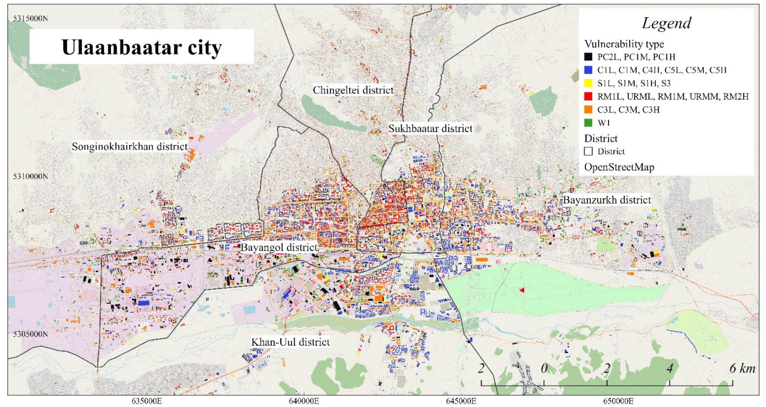
Figure 9 illustrates the distribution of the assigned building classes.
Figure 10 shows the vulnerability functions of the GAR-13 used in this study. The horizontal axis indicates a spectral acceleration in
g at the typical period for each building class shown in
Table 8. According to the vulnerability functions, a considerable repair cost is expected in unreinforced masonry buildings such as URML and URMM. Those vulnerability functions are used in the following seismic loss estimation.
3. Strong Ground Motion Prediction for a Scenario Earthquake
Strong ground motions in the target area for a scenario earthquake are estimated by the simulation techniques based on the stochastic Green’s function method (SGFM) and the equivalent linear seismic response analysis. The SGFM consists of a simulation of the ground motions generated from sub-faults (small events) [
24] in an anticipated large earthquake fault and a summation of the generated ground motions in the smaller events [
25,
26]. The method can create the synthesized strong ground motions at arbitrary sites on seismic bedrock (approximately shear-wave velocity of 3 km/s) and has been widely used in current strong ground motion predictions. In order to estimate the ground motions at the ground surface, site amplification of the surface soils needs to be considered. The authors already estimate the underground shear-wave velocity structure models at approximately 50 sites in the UB area by the inversion analysis of the observed microtremor data [
28]. We apply the equivalent linear seismic ground response analysis of DYNEQ [
27] to the estimated ground motions at bedrock and the shear-wave velocity models to consider the nonlinear response of strong shakings. Finally, we estimate the distribution of spectral accelerations for the scenario by interpolating the estimated ground motion intensities.
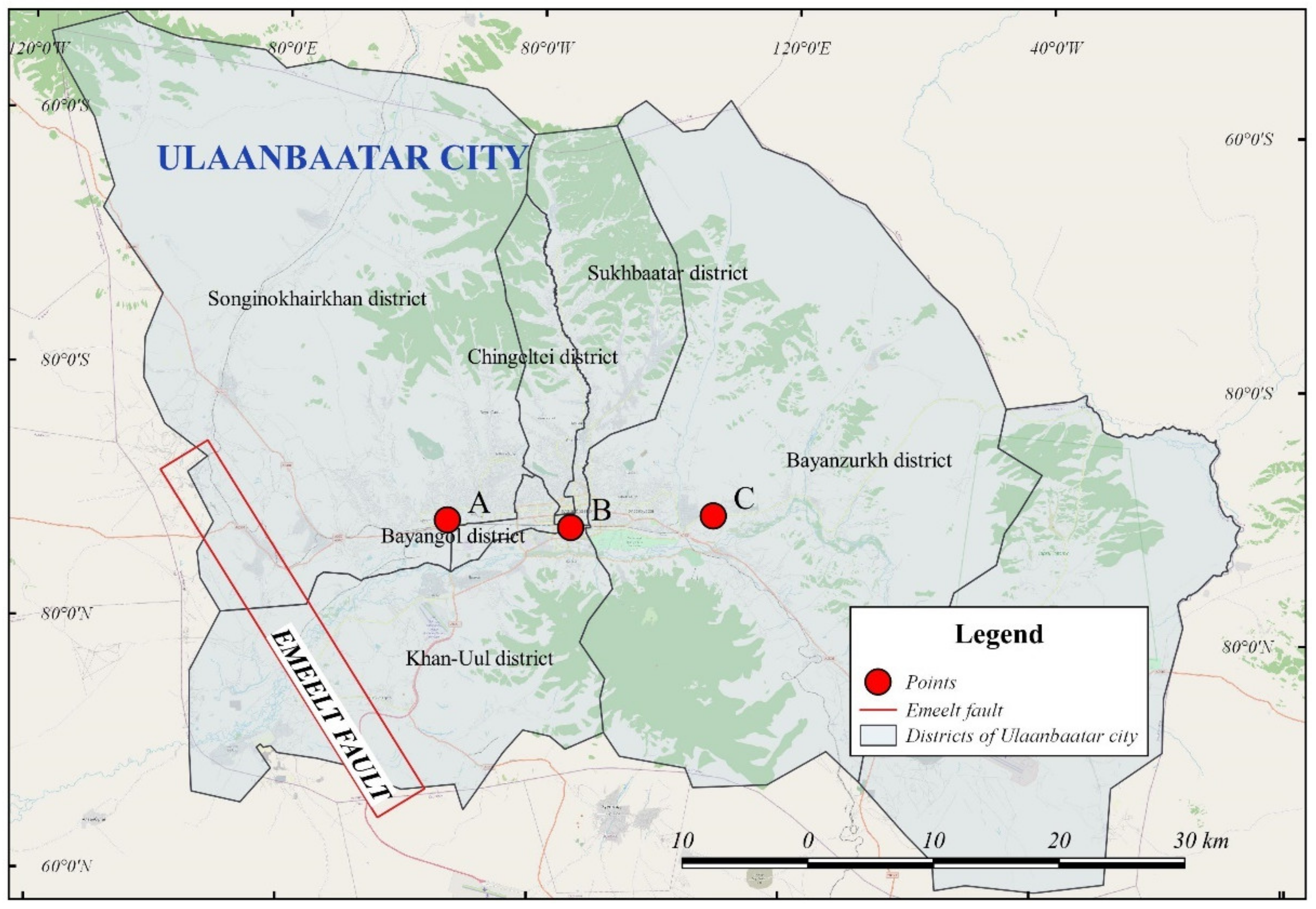
We selected the Emeelt fault as the scenario earthquake because the fault is located only 20 km from the central UB area.
Figure 11 shows the location of the Emeelt fault, and
Table 9 shows the parameters of the characterized fault model of the scenario earthquake. The fault location, orientation, and the detailed fault parameters proposed in the previous study [
33] are used in the simulation.
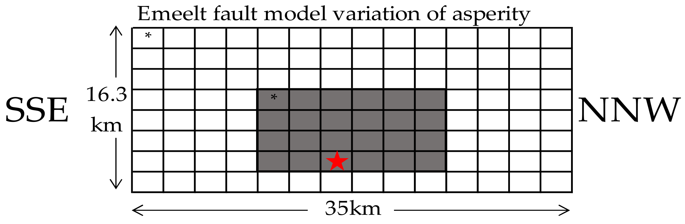
Figure 12 shows the Emeelt fault characterized variation model, which is estimated as the severest scenario. The expected moment magnitude (Mw) is 7.4, and one asperity, also known as strong motion generation area, [
26] is assumed in the earthquake. The path and site properties used in the SGFM are also listed in
Table 9. We simulated the strong ground motions at 50 sites where the shear-wave velocity models were obtained in our previous study [
28]. The upper figures of
Figure 12 show the time histories of acceleration waveforms on the seismic bedrock estimated by the SGFM at the site A–C in
Figure 10. Since we assume a constant radiation pattern, only one horizontal component of the seismic wave is estimated at each target site.
In order to evaluate the nonlinear seismic ground response, the equivalent linear response analysis of DYNEQ [
27] is applied in this study. DYNEQ is an open-source program that considers the strain-dependent soil properties (shear modulus and damping factor) of horizontally layered media during strong shaking. DYNEQ can also consider the frequency-dependent dynamic soil properties to suppress the underestimation of short-period surface ground motions that were sometimes found in applying the SHAKE [
34]. The shear-wave velocity models estimated in our previous study [
28] are used in the simulation. We assume all the soil layers in the UB area as sand and gravel and apply the soil properties introduced in Refs. [
35,
36].
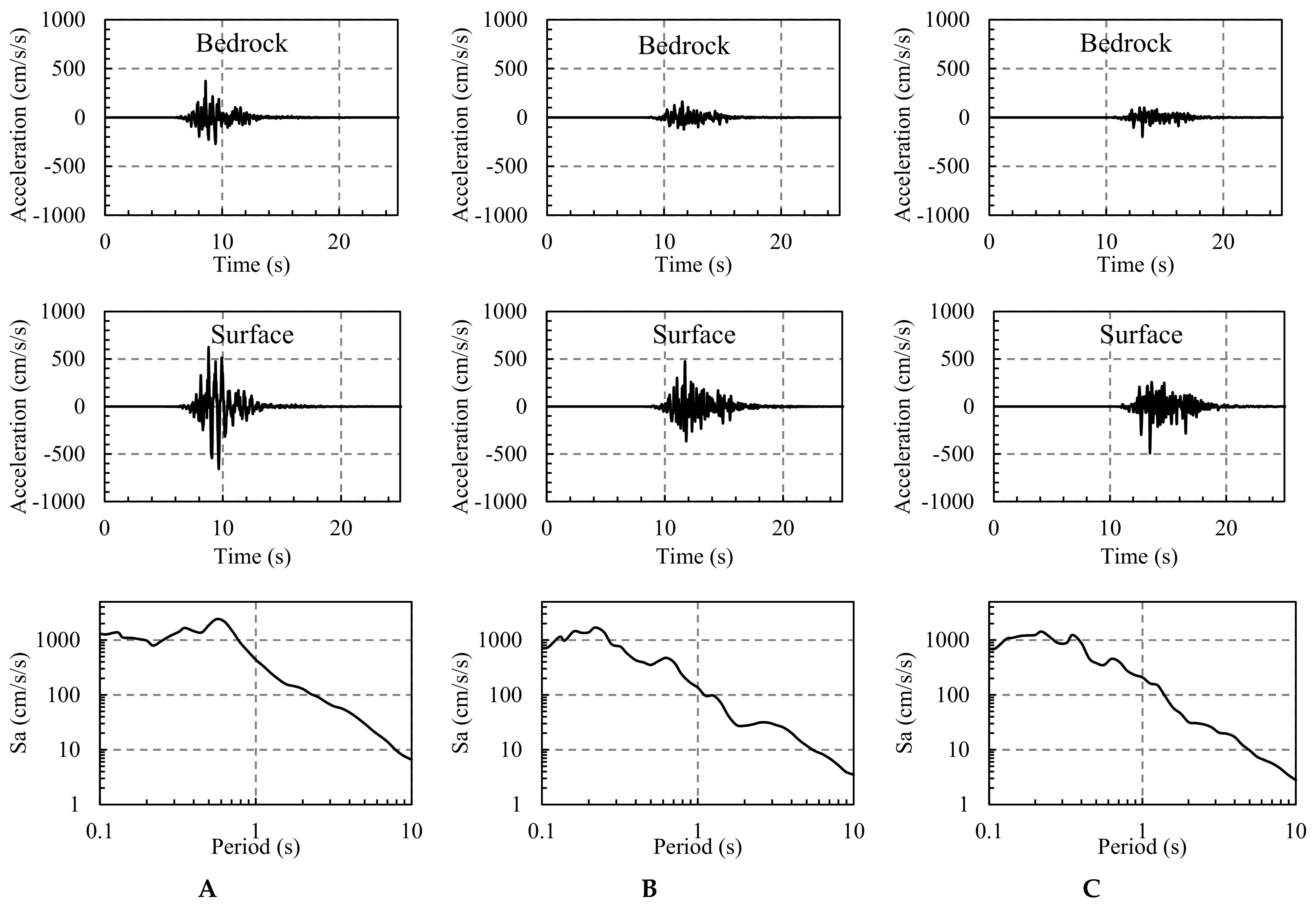
Figure 13 shows the estimated surface ground motions and acceleration response spectra at sites A–C. The peak ground acceleration (PGA) at site A located closer to the earthquake fault is approximately 700 cm/s
2, and the PGAs at sites B and C in the central and eastern part of UB are about 500 cm/s
2, respectively. A significant peak is found at 0.6 s in the response spectrum at site A. Multiple peaks are found at 0.25 s and 0.7 s in sites B and C.
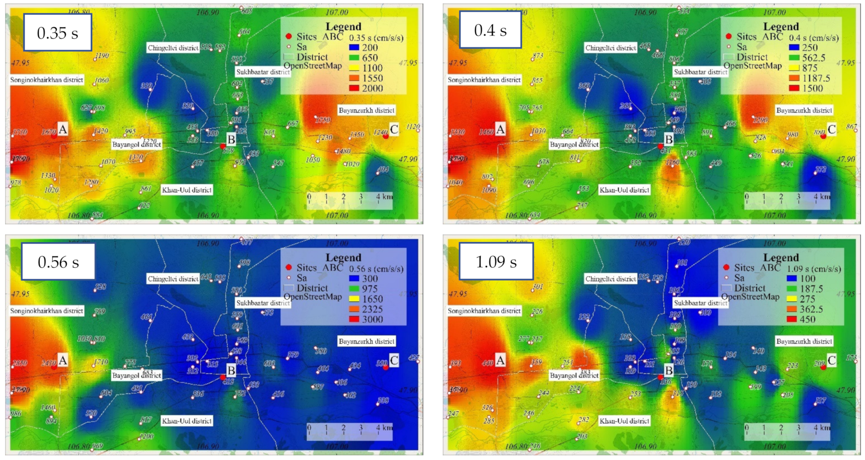
In order to accurately assess the vulnerability for building-by-building, strong motion at each building site needs to be estimated. However, it is challenging to estimate ground motions at arbitrary sites because of the limitation of the available sites where the shear-wave velocity model is obtained. Therefore, the spatial interpolation technique is applied to estimate the distribution of response accelerations. The inverse distance-weighted interpolation (IDW) is used in this study.
Figure 14 shows the distribution of the response accelerations in UB for the typical periods (0.35 s, 0.40 s, 0.50 s, and 1.09 s). Larger accelerations are estimated in the western area because of the closer distance to the earthquake fault. On the other hand, large accelerations at 0.35 s and 0.40 s are also estimated in the eastern area, although the area is farther than the central area to the fault. According to our site effect assessment [
28], strong amplifications in short periods were expected in the eastern area, probably due to the soft deposits along the river.
4. Seismic Loss Estimation
The economic loss of the buildings by the scenario earthquake is estimated by the simulated response spectral accelerations, the vulnerability functions, and the construction costs estimated in
Section 2.
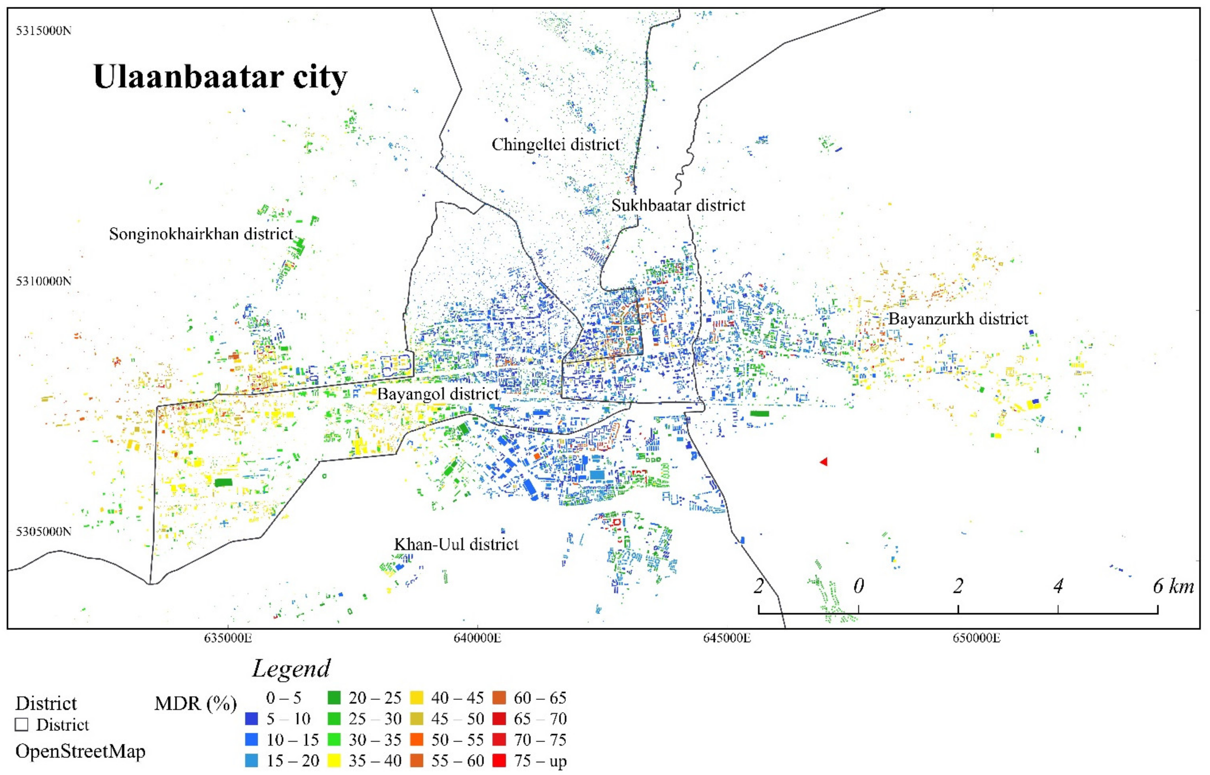
Figure 15 shows the distribution of the estimated MDRs in the percentage of each building. Higher MDRs than 50% are estimated in the western and eastern part of the UB area, whereas the MDRs in most of the buildings in the central area are lower than 20%.
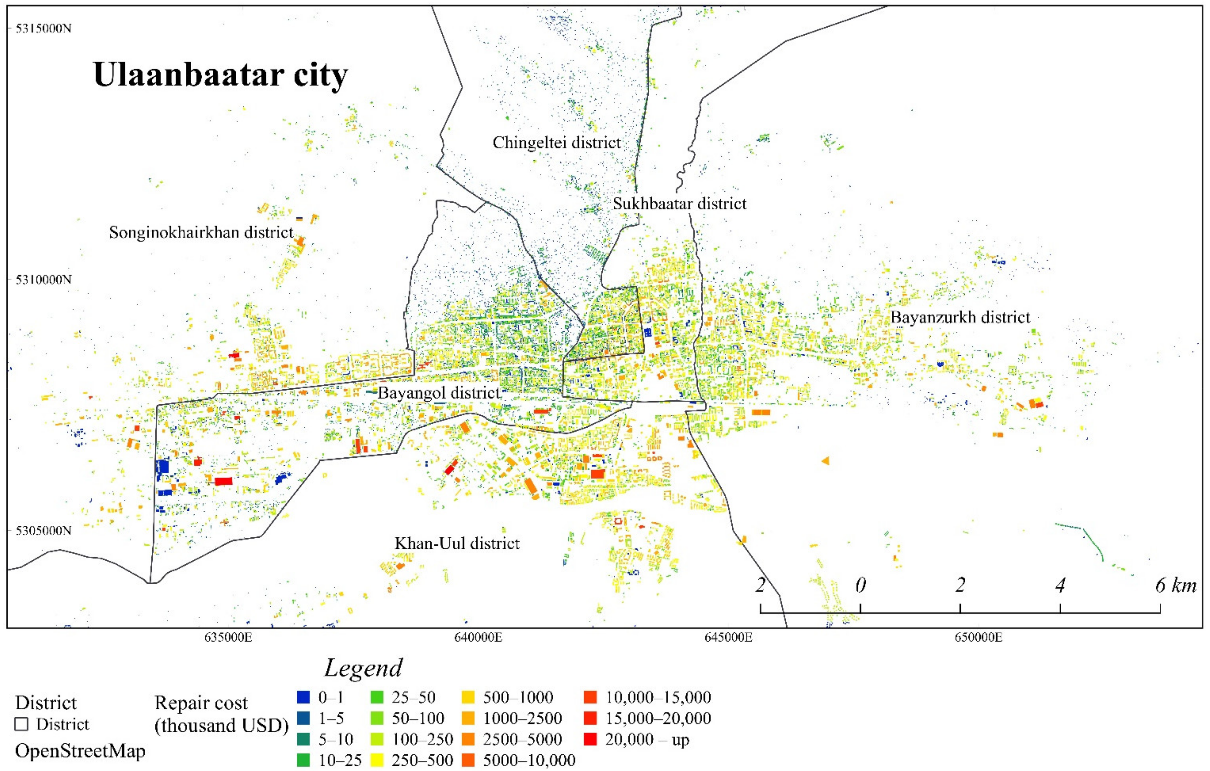
The repair costs of the buildings are estimated from the construction costs by multiplying the MDRs shown in
Figure 10.
Figure 16 shows the distribution of the expected repair costs of the buildings in thousand USD for the scenario. The repair costs for most of the buildings are lower than 20,000 USD. Those buildings correspond to the small low-rise masonry buildings. Higher repair costs are expected in more significant buildings, especially in the southern part of the UB area, because high-rise residential apartment buildings have become concentrated in recent years.
In the updated building inventory data, the total amount of the construction cost for the buildings in UB is approximately 28.7 billion USD. The result of the loss estimation shows that the total amount of repair costs for damaged buildings is approximately 3.4 billion USD in the scenario. According to the economic situation by The World Bank [
37], the average of the recent 5-year growth domestic product (GDP) in Mongolia is approximately 13 billion USD. It indicates that the total direct losses of the buildings in the scenario correspond to approximately 26% of the Mongolian GDP. Jaiswal and Wald [
38] estimated the direct shaking-related economic losses in the recent worldwide M7 class earthquakes as 3.0 billion USD for the Haiti earthquake on 12 January 2010 (M7.0), 2.0 billion USD for the Canterbury, New Zealand earthquake on 3 September 2010 (M7.0), and 2.0 billion USD for the Eastern Turkey earthquake on 23 October 2011 (M7.1), respectively. Whereas our estimation’s seismic and urban conditions are different from those in the previous earthquakes, our estimated economic loss is consistent with those in the earthquakes. If indirect losses such as business interruption are counted in the loss estimation, many more significant losses would be expected. In order to reduce the building damage and losses, seismic retrofitting and structural rehabilitation, especially for non-engineered buildings such as unreinforced masonry, would be substantial.
5. Conclusions
In this paper, we introduced an algorithm for estimating the construction cost of buildings from GIS building inventory data in Ulaanbaatar city (UB), Mongolia. We estimated building losses due to a scenario earthquake. Although the building inventory data are available in UB, information on the structural type and construction year were not registered in some buildings. We estimated the structural type and construction year by applying the criteria based on the building characteristics in the existing inventory data. We confirmed that the estimated structural types show good agreement with the actual buildings. The construction costs of the UB buildings are calculated based on the updated building inventory data and the Mongolian construction code. The vulnerability functions of GAR-13 were also assigned to the buildings considering structural type, building height, and construction year.
Strong motion simulation for the scenario earthquake by the Emeelt fault was performed using the stochastic Green’s function method and the equivalent linear ground response analysis. The shear-wave velocity models estimated by the previous authors’ research were used in the seismic response analysis. The peak ground accelerations for the scenario were estimated at more than 500 cm/s2 in UB, with especially larger accelerations expected in the western area located closer to the fault. By using the construction cost inventory, the vulnerability functions, and the simulated response accelerations, the expected repair costs of the damaged buildings were estimated. The direct loss of the buildings reached a total of 3.4 billion USD in the target area, which corresponds to approximately 26% of the recent GDP in Mongolia. The developed inventory database and the procedure for the seismic loss estimation would be useful for considering countermeasures against future earthquake disasters for the national government and local municipalities.
The strengths of our approach can be summarized as the monetary loss of damaged buildings can be estimated not only for scenario earthquakes but also for an actual earthquake by using our developed building inventory. Generally, it would be complicated to estimate the total amount of loss immediately after an earthquake. Our developed approach can produce a damage distribution map and amount of building loss immediately after an earthquake if ground motion data are available. In addition to the wider-practical aspect and value of the performed study, the obtained data can be applied in the earthquake insurance market for assessing building stocks in UB.
On the other hand, the limitations of our approach can be summarized as the applicability of the vulnerability functions, the accuracy of the seismic ground motion prediction, and the quality of building inventory data. Although we used the global vulnerability functions proposed in GAR-13, the applicability needs to be discussed by considering the actual seismic capacity and dynamic characteristics, including natural periods of UB buildings. Since detailed shear-wave velocity structure models in UB are not available yet, we applied a one-dimensional ground response analysis in the seismic ground motion prediction. If a more detailed Vs-model was to be available by future dense geophysical explorations, 3D ground motion simulation techniques such as the finite difference method could be applied to estimate not only body waves but also basin-induced surface waves. Finally, the building inventory data of UB still has uncertainties in heating types, structural types, and construction years because it was challenging to determine them from the currently available data accurately. Updating the inventory data would be one of the important issues for a more reliable earthquake loss assessment in UB.


