
A Method to Identify Urban Fringe Area Based on the Industry Density of POI
by
 , and
, and
Qi Dong
1,2,3,4, 
Shuxue Qu
1,2,3,4,
Jiahui Qin
1,2,3,4,
Disheng Yi
1,2,3,4,
Yusi Liu
1,2,3,4 and
Jing Zhang
1,2,3,4,* 1
College of Resources Environment and Tourism, Capital Normal University, Beijing 100048, China
2
Beijing Laboratory of Water Resources Security, Capital Normal University, Beijing 100048, China
3
3D Information Collection and Application Key Lab of Education Ministry, Capital Normal University, Beijing 100048, China
4
Beijing State Key Laboratory Incubation Base of Urban Environmental Processes and Digital Simulation, Capital Normal University, Beijing 100048, China
*
Author to whom correspondence should be addressed.
ISPRS Int. J. Geo-Inf. 2022, 11(2), 128; https://0-doi-org.brum.beds.ac.uk/10.3390/ijgi11020128
Submission received: 3 November 2021
/
Revised: 4 February 2022
/
Accepted: 9 February 2022
/
Published: 11 February 2022
(This article belongs to the Special Issue Geo-Information for Developing Urban Infrastructures)
Abstract
:During the period of rapid urbanization, the urban fringe area is the area where urban expansion occurs first, and land use change is the most active. Studying its evolution laws and characteristics is of great significance to urban planning and urban expansion, and the primary task of fringe area research is the spatial recognition and boundary division of urban fringe area. The previous methods for defining urban fringe areas are mainly divided into qualitative division based on experience and quantitative division based on indicators constructing. This research avoids the construction of index systems and the selection of mathematical models and improves the objectivity of the experiment. Based on the existing methods, this research considers the correlation between the difference of industrial distribution within cities and the urban spatial structure and spatial distribution of urban elements and considers the distance decay law of urban density. The urban fringe area in this research is defined as the distinction region of the service and manufacturing industry extending outward from the inside of the city. First, calculate the POI density of service industry and manufacturing industry. Then look for the inflection point where its density value drops sharply and get the isoline of that point. The range within the isoline is that the industry extends outward from the inner city and has reached the saturation state. Two types of industries can determine two isolines, and the belt region between those isolines is the urban fringe area. We use the urban fringe area identified from the impervious surface data to verify the result. The comparative results show that the identification method of urban fringe area based on POI works effectively, and it can successfully identify the multi-center urban core area. The method mentioned in this paper provides a new idea from the perspective of industrial activities in identifying and defining the belt region of urban fringe area.
1. Introduction
Urbanization, as a universal social phenomenon in the world, is mainly manifested as the expansion of urban land area and the extension of human activities. The process of urbanization profoundly changes the surface system of the earth, which is directly manifested as the expansion and spread of urban construction land in regional space, and leads to a series of land use and cover changes and natural environment disturbances [1]. Under the influence of this process, the characteristics of urban and rural areas become more similar, and the boundary between urban and rural areas becomes more blurred, which leads to the proposal of the theory of urban fringe area. Urban Fringe is a transitional zone between Urban and rural areas with both Urban and rural land use properties. It represents the area where urban expansion and industrial development first occur. The most widely used definition of urban fringe is proposed by Pryor [2] “a zone of change in land use, social and demographic characteristics, located in a land use conversion area between contiguous built-up areas and suburbs and a pure agricultural hinterland almost completely devoid of non-agricultural housing, non-agricultural occupation and non-agricultural land use”. As the carrier of urban expansion, the urban fringe area is also the distribution center of material and energy exchange between the city and external regions. It has become the most sensitive area with the largest, fastest and most rapid changes in common sense space [3].
Although the urban fringe is an objective regional entity, the transition and complexity of the fringe itself, as well as the dynamicity and fuzzification of the boundary lead to a long-term debate on the scope division of the urban fringe in academia, and it is difficult to form a unified theory and method. In early foreign studies, it is more common to divide the marginal area based on experience. For example, Friedman [4] divides the area about 50 km around the city into urban fringe areas according to the daily commuting area of people, of which the inner fringe area is about 10~15 km, the outer fringe area extends 25~50 km. In the follow-up research, people prefer to replace it with a quantitative method. Therefore, Russwurm [5] uses the ratio of non-agricultural population to agricultural population to define the urban fringe area, pointing out that the area with the ratio less than or equal to 0.2 is rural, the semi-agricultural area is between 0.3 and 1.0, the semi-urban area is between 1.1 and 5.0, and the urban area is greater than 5.0. The formation background and dynamic mechanism of urban fringe in China are different from those in foreign countries. On the basis of drawing lessons from relevant researches, domestic scholars have made abundant explorations on the scope of urban fringe in China. The first is based on administrative boundary. Gu et al. proposed that the inner boundary of urban fringe should be bounded by streets, the basic administrative units of urban built-up areas, and the outer boundary should be bounded by the diffusion range of urban material elements [6]. The second is to construct an index system, which is defined by a mathematical model. Gu et al. used the population density index and took the street as the basic unit to make a quantitative analysis of Shanghai’s urban fringe areas [7]; Chen constructed 5 categories of 20 indicators, and used the “break point” method to find the mutation value of the distance attenuation of each element, and defined the urban fringe area of Beijing [8]; Cheng and Zhao applied remote sensing technology and the principle of information entropy to explore the boundaries of Beijing’s urban fringe zone [9]; Li proposed the concept of the attributes of the geographic characteristics of the fringe area of a big city, that is, the degree to which the comprehensive characteristics of a specific geographic unit in the fringe area of a big city belong to the city, and proposed a method for defining the regional characteristic attributes of the fringe area of big cities based on fuzzy comprehensive evaluation [10]; Zhang et al. and others extracted urban land use information from TM images, and applied the “mutation detection method” to divide the urban fringe area of Beijing [11]; Cao et al. used non-linear regression, spatial autocorrelation and GIS to determine the inner and outer boundaries of urban fringe areas by looking for mutation points in the spatial distribution characteristics of the service industry and manufacturing industry [12]; Wang et al. put forward the concept of urbanization characteristic attributes, and used a logistic regression model to classify urban fringe area [13]. The above methods have disadvantages such as strong subjectivity, non-unique model selection, difficulty in obtaining high-precision remote sensing data, and large differences in remote sensing interpretation results.
The arrival of the era of big data provides new ideas and methods for the study of urban boundaries, and the data with geographical location information provides a new perspective on the study of urban spatial structure. Among them, point of interest (POI), as a carrier of location information and attribute information, is significantly better than population density data and remote sensing data in terms of update speed and accessibility. Its characteristics of fast dynamic update and perfect economic and social attributes can help to establish a mapping system from POI to industrial type data and explore the characteristics of urban spatial structure from multiple perspectives such as industry aggregation, development orientation, and functional division. The relationship between POI and urban activities is mainly reflected in the distribution characteristics of POI directly reflect the texture of the city and the gathering activities of various urban activities, so it can reflect the urban structure in space; secondly, the spatial distribution difference of POI density reflects the different regional development level [14]. In the same city, the degree of regional development is often proportional to the density of POI. In different cities, the density of POI reflects the degree of urbanization. In addition, the differences in the types and quantities of POI also reflect the differences in urban functions to a certain extent.
From a long-term perspective, urban expansion is a dynamic process of rolling outward expansion. The plane mapping of the urban area is the static section of the urban area at this stage. From this, it can be seen that in the process of urban expansion, the distribution of industries presents certain spatial characteristics. Regarding the evolution process of urban fringe area, urban fringe area is expressed as a dual process of urban suburbanization and suburban urbanization in urban geography [15]. The industrial characteristic of the process of urban suburbanization is that the process of manufacturing suburbanization occurs before the service industry [16], the manufacturing industry is distributed in the periphery of the service industry. The industrial characteristic of the process of suburban urbanization is that the manufacturing industry develops first, the proportion of agriculture declines, the service industry rises steadily, and the service industry is concentrated in the city center [17]. The specific performance of this theory is: due to factors such as land price, transportation, pollution, etc., compared with the service industry, the manufacturing industry always tends to choose locations in the outskirts of cities with open terrain, low land prices and convenient transportation in the initial stage of expansion. After a certain stage of development, with the growth of population density and the improvement of public facilities, the service industry has gradually developed, and the development speed is faster than that of the manufacturing industry, but the scope of development is smaller than that of the manufacturing industry. Compared with the manufacturing industry, the location of the sudden decrease in industrial density is significantly closer to the city center. The extreme point of industrial density change scales the sudden change between urban and rural areas. From the city center to the outside, the density of the service industry gradually decreases, and the point of sudden change can be considered as the internal fringe of the urban fringe area. The density of manufacturing industry shows the characteristics of increasing first and then decreasing, and the sudden change point of its rapid decrease can be regarded as the external fringe of the urban fringe area. Therefore, the main problem of this study is to find the extreme points of the industrial density change of the service industry and the manufacturing industry, so as to mark the two boundaries of the urban fringe area.
In view of this, we take the description of urban fringe area in urban geography as a theoretical basis, consider the dual processes of forming urban fringe areas, take density analysis as the method, and use POI data to find boundary thresholds to identify the extent of urban fringe areas, and provide help for understanding and analyzing cities. Compared with the previous methods, this method completes the connection between spatial attributes and socio-economic attributes by using POI dataset and reflects the urban spatial structure with industrial structure on the basis of considering the dual characteristics of urbanization process, through this method, we obtain the urban fringe area that is not restricted by the grassroots administrative area and can better identify multiple urban sub-centers in the process.
The remainder of this paper is structured as follows. After summarizing the previous studies and the limitations of them, the research ideas and writing logic of this paper are briefly introduced. Section 2 describes the research area and data source. Section 3 mainly introduces the methods and principles used in the research. Firstly, the principle of adaptive kernel density is explained, which is applied to the calculation of bandwidth after considering the influence of local outliers. Secondly, Densi-Graph threshold determination method is introduced, which is also the main method to determine the density threshold. Then a grid-based urban land extraction method for testing is introduced. In Section 4, the methods introduced in Section 3 are used to conduct empirical research and verification on Beijing. After comparing with existing urban built-up areas, the differences were explained by combining POI types. Finally, the experimental results are discussed and summarized.
2. Study Area and Data Source
2.1. Overview of the Study Area
The study area is Beijing, including 16 municipal districts: Dongcheng District, Xicheng District, Chaoyang District, Fengtai District, Shijingshan District, Haidian District, Shunyi District, Tongzhou District, Daxing District, Fangshan District, Mentougou District, Changping District, Pinggu District, Miyun District, Huairou District and Yanqing District. The overview of study area is shown as Figure 1. According to the web of the people’s government of Beijing municipality (http://www.beijing.gov.cn/renwen/bjgk/ (accessed on 2 November 2021)), Beijing is mainly located at 39.9-degree North latitude and 116.3-degree East longitude. It covers an area of 16,410.54 square kilometers and has a permanent population of 21.89 million.
2.2. Experimental Data and Preprocessing
2.2.1. Point of Interest
The data used in this paper is the POI data of Beijing in 2016 collected through the API of Baidu Map, with a total of about 300,000 pieces of data. Data attributes include ID, longitude, latitude, name, address, label, first class classification and second-class classification. After coordinate transformation, two attributes of transformed longitude and transformed latitude are added. The data properties are shown in Table 1. After dividing POI according to industry types, the dataset is divided into two categories: service and manufacturing. The service industry includes catering, shopping, educational institutions, leisure and entertainment, life services, automobile services, hotels, finance, etc. The manufacturing industry includes factories and mines, industrial parks, agriculture, forestry, fishing and animal husbandry related industries, furniture manufacturing, high-tech industrial parks, etc.
2.2.2. Global Artificial Impervious Area (GAIA)
The global artificial impervious area data used for verification in this paper are from the Global Land Cover Finer Resolution Observation and Monitoring Data Platform of Tsinghua University. In 2020, The scientific research team of Professor Gong, Department of Earth System Science, Tsinghua University released the global long-term time-series dynamic land cover data product (GLASS-GLC), and in the same year released the finer resolution (30 m) global artificial impervious area annual dynamic data product (1985–2018) (GAIA) [18]. This dataset was based on Landsat remote data and other auxiliary data (night light data and Sentinel-1 radar data) over a long time series. First, rapid mapping of annual impervious surface was realized through the exclusion-inclusion algorithm. Then temporal consistency check algorithm was used to filter the initial impervious surface sequence and transform logic reasoning, so as to ensure the rationality of the obtained impervious water surface sequence in time and space. The artificial impervious area data of Beijing in 2016 were obtained after the extraction of Beijing area.
3. Methods
3.1. Adaptive Kernel Density Estimation Based on LOF (LOF-AKD)
In this study, the kernel density estimation method was selected to quantitatively describe the aggregation degree of POI. The kernel density estimation method takes into account the location factor of the first law of geography, that is, the kernel density value of the position with dense surrounding points is high, and the kernel density value of the position with sparse surrounding points is low. In order to measure the aggregation of point elements, the kernel density estimation method was used to calculate the kernel density of each point of interest, and the value of the kernel density at this point reflects the concentration degree of points at this point [19]. In this paper, referring to the local outlier detection method proposed by Xie and Tang [20], and using the degree of outlier of points to reflect the degree of aggregation of point sets, the adaptive kernel density method (LOF-AKD) based on local outlier factors is proposed.
LOF-AKD algorithm is the application and improvement of LOF algorithm. Here we first give some basic definitions of LOF algorithm, and then introduce the implementation of LOF-AKD algorithm in detail.
3.1.1. LOF Algorithm
LOF (Local Outlier Factor) is a density-based local outlier detection algorithm. The core idea of LOF is to calculate the local reachable density of data objects, and use its neighborhood within the scope of the local can be up to the average density of all other objects with their own local to the ratio of the density value to indicate the degree of outlier data objects, this ratio is called local outlier factor, reflecting the data object is distributed in local area and its density is relatively similar [20]. The key step of LOF algorithm is to determine whether the data point is an outlier by assigning an outlier factor LOF that depends on the neighborhood density to each data point. If LOF >> 1, the data point is an outlier; if the LOF is close to 1, the data point is a normal data point and distributed in a local range close to its density. If LOF < 1, it indicates that the density of the data point is higher than that of its neighborhood points. The definition of LOF algorithm is as follows:
Definition 1.
The K-distance of point O(K-distance(O)): In point set S, the distance d (O, Si) of the Kth farthest point Si from point O is denoted as K-distance (O), where , and satisfies:
- (1)
- There are at least K objects, such that;
- (2)
- There are at least K-1 objects, such that
Definition 2.
The K-neighborhood of point O((O)): In the point set S, O ∈ S, given the K distance of point O, the K-neighborhood of point O is all points in the range of K distance (including K distance) of point O, that is:
So the number of neighborhood points .
Definition 3.
The reach_distance from point O to point si(reach_distance k(O,si)):
In point set S,, the reach_distance from point O to point si is:
Definition 4.
The local reachable density of point O(lrd(O)): In point set S,, the local reachable density of point O is:
It is the reciprocal of the average reachable distance from point O to point p in the K-neighborhood of point O.
Definition 5.
The local outlier factor of point O(LOF(O)): In point set S, O ∈ S, then the local outlier of point O is:
Represents the average ratio of the local reachable density of the neighborhood point ( of point O to the local reachable density of point O.
3.1.2. LOF-AKD Algorithm
Kernel density estimation is a nonparametric method for estimating the probability density function. The idea is to use a smooth peak function for the point (i = 1, 2, 3 ……, n) to carry out smooth extension and fit each point into a smooth probability density surface. In centered, in order to determine its bandwidth h for radius of the area, highest probability, the probability of each location point in the area of value with the attenuation distance and , making and center distance near the location of the point are endowed with higher probability, at a distance equal to the bandwidth is 0, the location of the point probability by superimposing space elements of the probability density at all points, The spatial distribution characteristics of point density are high in the aggregation region and low in the discrete region [15]. The kernel density estimation formula is as follows:
The K (.). Is the standard Gaussian kernel function, as shown in Equation (6).
Kernel density bandwidth h represents the smoothing range of each point. For a fixed-point set, if the bandwidth is too large, an overgeneralized continuous region will be obtained, with obvious global features but weak local features. If the bandwidth selection is too small, a number of relatively fine discrete regions will be obtained, with obvious local features but weakened global features. Therefore, the selection of bandwidth should be adapted to the degree of discreteness of point sets, that is, the size of bandwidth should be positively correlated with the degree of discreteness of local point sets. For dense point sets, a smaller bandwidth should be selected, while for sparse point sets, a larger bandwidth should be selected, so that the local and global features will not be excessively highlighted or weakened [19].
We mainly think about the kernel density estimation method from two aspects, adding the local outlier factor to the density measurement:
The average reachable distance in the LOF algorithm is used to replace the traditional distance in the kernel density estimation formula to better reflect the neighborhood features, especially the density features, near the points. The formula of average reachable distance is as follows:
In the selection of bandwidth, the adaptive bandwidth reflects the degree of dispersion of the local point set, and the size of the bandwidth should be proportional to the degree of dispersion of the point set. It is compared to the local outlier factor LOF. LOF < 1 and LOF close to 1 reflect the aggregation of the point set, and LOF > 1 reflects the dispersion of the point set. Therefore, LOF is used as an indicator to determine the adaptive bandwidth, at the same time, considering the divergence characteristic of the bandwidth function, the bandwidth function is determined as:
3.2. Densi-Graph Threshold Determination Method
After calculating the kernel density values by the above adaptive kernel density estimation method, we found that the difference in kernel density values can reflect the difference in the extension range of the service industry and the manufacturing industry. Generally speaking, the extension range of the manufacturing industry is larger than that of the service industry in a city. Therefore, we need to find an area with both urban and rural characteristics, where services are relatively sparse and manufacturing is relatively intensive. The problem then turned to finding areas where the nuclear density values of the two industries had suddenly changed. In this case, it is necessary to determine the threshold inflection point of kernel density contour line from dense to sparse. In this paper, the Densi-Graph threshold determination method proposed by Xu and Gao based on Point of Interest (POI) data is used to identify the boundary of urban built-up areas [21]. The basic idea is as follows: In order to find the threshold inflection point of the isoline from dense to sparse, the expression that can describe the density of the kernel density isoline should be found first. To solve this problem, Xu used the theoretical radius difference of the closed graph enclosed by adjacent isolines to describe the density of the isoline. In order to quantify the density, Densi-Graph was plotted by the difference of theoretical radius between the closed Graph formed by kernel density value and corresponding isoline. In the urban space, the distribution law of POI is as follows: the closer to the urban center, the larger number of POI, density and aggregation characteristics are more obvious; Therefore, the general spatial distribution characteristics of the kernel density isolines of POI are as follows: in the urban center, the isolines are closely spaced; In the outskirts of the city, the distance of contour lines gradually enlarges; at the boundary between urban and rural areas, the distance of contour lines will increase sharply. In order to obtain the threshold value of this sudden change region, is defined as the theoretical radius of the closed graph surrounded by isolines, where is the area of the closed graph, and the derivative of the increment of the theoretical radius is obtained by taking the corresponding kernel density value as the abscissa. When the first derivative approaches 0, it indicates that the distribution of kernel density isoline is uniform, that is, the urban space expands evenly and there is no boundary with the countryside. When the first derivative is greater than 0, it indicates that the kernel density isoline gradually diverges outward, that is, the urban development is uneven, and the so-called urban-rural boundary appears. As shown in Figure 2, it can be seen that the density difference of POI results in different density of corresponding contour lines. The ideal state of this situation is shown in Figure 3. It can be clearly seen that the distance between two contour lines is significantly larger than before, corresponding to Figure 4, which represents the threshold value where the slope suddenly increases. By differentiating the first derivative, the inflection point of the density isoline can be obtained, and by discriminating the global inflection point, the key point of regional spatial structure change can be found, that is, the threshold value of the boundary of urban built-up area.
3.3. Extraction of Urban Land Use Information Based on Grid
The verification method used in this paper is based on the sliding window detection method in the urban fringe area definition method based on the theory of regional urban structure and remote sensing monitoring by Mu et al. [22] The detection process mainly uses two methods: index calculation method and structure division method. The main idea of index calculation method is to take the proportion of urban land as the index of urban structure division. The urban land use ratio is defined as follows: In a pixel window of a certain size, the ratio of urban land use pixel to total pixel is the urban land use ratio of the pixel in the center of the window. When calculating the proportion of urban land, urban land is firstly extracted from remote sensing image to obtain the urban land distribution map. Then, the proportion of urban land is calculated by window smoothing operation. A window of a certain size is opened on the urban land distribution map, and the proportion of urban land area in the window to the entire window area is counted, which is assigned to the center pixel of the window. Slide the window on the urban land distribution map by row and scan the full image to get the urban land scale map. The proportion calculation formula is as follows:
where D(i, j) is the proportion of urban land use, N is the window size, g(i, j) is the gray value of a pixel on the urban land use distribution map, and I and j are the number of corresponding rows and columns. If the pixel is urban land use, then g(i, j) = 1; otherwise, g(i, j) = 0. D(i, j) is the proportion of urban land use in pixel center of window, and the value is between 0 and 1. The structural division method means that the study adopts the natural segmentation point classification method to divide the urban land scale map into four categories. The proportion from high to low corresponds to the urban core area (urban land use ratio is 65–100%), urban fringe area (urban land use ratio is 34–65%), urban influence area (urban land use ratio is 13–34%) and rural hinterland (urban land use ratio is 0–13%). After the re-classification, the urban fringe is extracted from the urban structure. The natural segmentation point method is a data classification method used to determine the best combination of values into different categories. It uses iterative algorithm to search for segmentation points, which minimizes the difference between data values of the same type and maximizes the difference between different types, so as to achieve optimal classification.
3.4. Hierarchical Clustering
In order to further explore the industrial characteristics of the urban fringe areas, we adopt the method of hierarchical clustering to classify the urban fringe areas according to the industrial structure, so as to describe the characteristics more systematically and comparatively.
3.4.1. TF-IDF
TF-IDF (Term Frequency–Inverse Document Frequency), is a statistical method for the importance of text words. Considering that the frequency of occurrence of some important and special words in documents is not high, to better characterize the characteristics of this document, it improves the weight of the words by weighting, the calculation formula is shown in Equation (10). We use this method to extract industrial features of urban fringe areas in different municipal districts. The type of POI in urban fringe areas in each municipal district constitute a word, and one urban fringe area constitutes a document. After processing by this method, we can get the feature vector of each city fringe area.
In the formula: is the frequency of POI type i in the research unit dj, it is calculated by the ratio of the number of occurrences of this POI type in research unit , to the sum of the number of occurrences of all POI types in research unit . IDF is the inverse document frequency, which is calculated by taking the logarithm of the ratio of the total number of research units to the number of research units that contain the POI type .
3.4.2. Hierarchical Clustering and Evaluation of Clustering Indexes
Hierarchical clustering creates a hierarchical nested clustering tree based on the distance (similarity) between cluster elements. In this paper, we use the hierarchical clustering method to perform the feature clustering of the urban fringe area. After obtaining the industrial type characteristics of each urban fringe area, we construct a clustering tree for classification by the bottom-up agglomeration method [23,24]. This method first treats each cluster element as a cluster, then calculates the distance between any two clusters, merges the two nearest clusters, and iteratively processes until all clusters are merged. The distance index is measured by cosine similarity [24]. To overcome outliers, the average distance is used for the inter-cluster distance.
After clustering, we use three evaluation metrics: Silhouette Coefficient (SC) [25], Davidson Burgin Index (DBI) [26], Calinski-Harabasz (CH) [27] to evaluate the clustering results. The larger the value of SC (Equation (13)), the better the clustering effect; the smaller the DBI (Equation (14)), the smaller the intra-class distance and the larger the inter-class distance, the better the clustering effect; the larger the value of CH (Equation (15)) is, the closer the class itself is, the more dispersed the classes are, and the better the clustering effect is.
In the formula, represents the average distance between the sample and all points in the cluster, namely the intra-class distance; represents the average distance between the sample and all the points in the nearest cluster, that is, the inter-class distance; is the total number of samples. is the average distance from the data within the class to the cluster centroid; is the distance between the centroid of cluster class and cluster class . is the trace of the inter-cluster scatter matrix; is the trace of the intra-cluster scatter matrix; is the number of clusters; is the center point of cluster ; is the center point of full sample data; is the number of samples of cluster .
3.5. Technology Roadmap
This study will be conducted on the basis of the following technology roadmap. The technology roadmap is shown as Figure 5. After the preprocessing of the experimental data, we use an adaptive kernel density algorithm which considers local outliers. The main idea is to reflect the degree of aggregation with quantized dispersion, so as to obtain the kernel density of points. Then, the contour line is generated according to the obtained density value, and the area surrounded by the contour line is statistically calculated. The Densi-Graph is generated according to the contour line value and the corresponding theoretical radius value. By searching for the threshold inflection point of the Graph, the corresponding contour line is determined as the obtained boundary. According to this route, we can get two boundaries, namely the external edge line and the internal edge line, and the part between them is the urban edge area.
4. Research and Results
4.1. Demarcation of Urban Fringe Area of Beijing
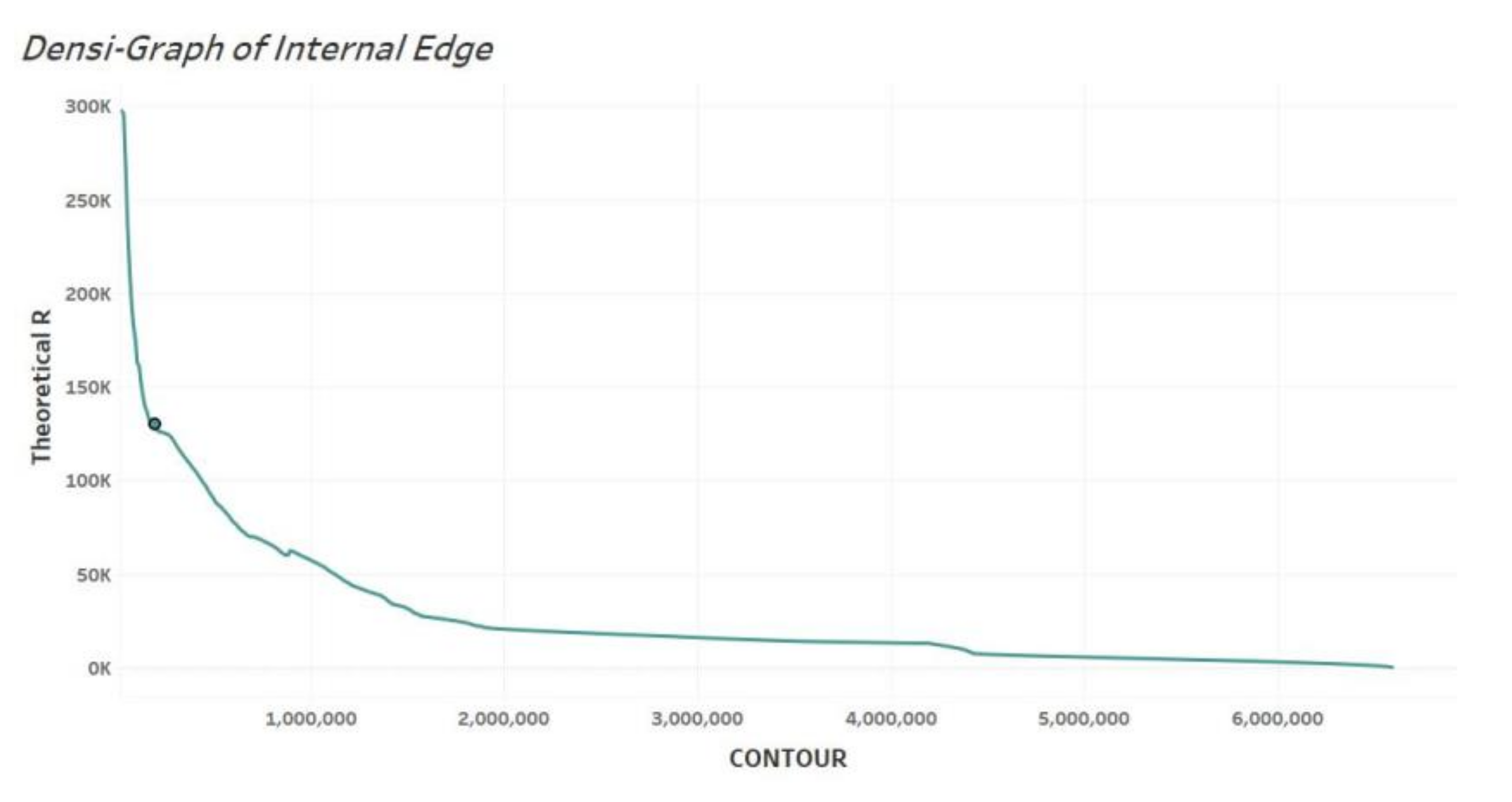
After preprocessing the POI data, the LOF-AKD method was used to calculate the kernel density of POI data sets of manufacturing and service industries respectively. As for the selection of K value in this method, K = 4, K = 10 and K = 20 were selected for the experiment based on the previous literature experience, and K = 10 was finally selected, that is, the kernel density value of each central point was calculated with the nearest 10 points around each central point as the calculation range. Contours are generated according to the kernel density value, and the kernel density contour of POI is an irregular closed curve with the highest point of urban POI density as the center (sometimes multiple centers) and expanding to all sides. For its spatial distribution characteristics, near the center of the density, the distance between the contour relatively close together, in the city periphery, the distance between the contour gradually expand, to the rural areas, the distance between the contour becomes very wide, which means contour of closed area from the city center to the city gradually increase, but this kind of growth is not uniform, That is, there is a threshold value to reflect the density from large to small, isoline from dense to sparse. According to the value of the isoline and the theoretical radius of the closed region S enclosed by the contour line, the fitting curve is the Densi-Graph, and the inflexion points of the two graphs are found by taking the derivative twice, which is the desired threshold. The Densi-Graph drawn is as follows:
The critical value of kernel density isoline from dense to sparse is determined as the threshold value of sudden change of POI density. The threshold boundaries determined according to the two types of POI are the two edge lines of urban fringe area, the internal edge line is defined according to the tertiary industry, and the external edge line is defined according to the secondary industry.
The abscissa of the two graphs from left to right indicates the trend of the density from low to high, reflecting the direction from the periphery to the city center. The critical value of kernel density contour from sparse to dense can be determined from the figure, which is the threshold of sudden change of the density. The threshold boundaries determined according to the two types of POI are the two edge lines of the urban fringe area. As Figure 6 and Figure 7 show, the internal edge line is defined according to the service industry (density value is 80,000), and the external edge line is defined according to the manufacturing industry (density value is 0.4).
Figure 8 shows the overall scope of the urban fringe area of Beijing. The blue line is the resulting internal edge, the red line is the resulting external edge, and the purple belt area between the two lines is the urban fringe area.
In the research results, from the perspective of administrative districts, we found that the traditional six districts of Beijing (Dongcheng District, Xicheng District, Chaoyang District, Haidian District, Fengtai District and Shijingshan District) basically did not include the urban fringe areas obtained in this study, except for Haidian, Fengtai and Shijingshan. The urban fringe area mostly appears on the side far away from the main center of Beijing, the urban fringe area of Haidian district and Fengtai District appears on the west side, and the urban fringe area of Shijingshan District appears on the northwest side, which not only represents the radiation effect of the main center of the city, but also shows the transition characteristics of Beijing from the city center to the suburbs. In addition, the results show that in addition to the six districts of central city, there are also small-scale urban sub-centers in Yanqing, Miyun, Pinggu, Huairou and Fangshan, and these sub-centers usually appear on the side close to the main urban center. The sub-center of Yanqing district is farther away from the main center than other urban sub-centers, so the urban fringe areas in Yanqing District are not connected with other urban fringe areas but distributed independently in the southwest of Yanqing District.
4.2. Verification Based on Artificial Impervious Area Data
We refer to the sliding window method to detect the proportion of urban land and superimpose the 1000 m ∗ 1000 m grid with the existing artificial impervious area data. It is undeniable that the smaller the grid, the more refined the spatial features will be, but at the same time, it will cause greater memory loss. In order to better express the spatial distribution features while having better operability, the 1000 m ∗ 1000 m grid is finally selected as the research unit. Then we use the spatial analysis method to count the proportion of artificial impervious area in each grid, and use the reclassification method to divide the grid into four categories according to the proportion of impervious water surface by natural segmentation method: urban core area (the ratio of artificial impervious area is 78~100%), urban fringe area (the ratio of artificial impervious area is 51~78%), urban influence area (the ratio of artificial impervious area is 23~51%) and rural hinterland (the ratio of artificial impervious area is 0~23%). The grids with extraction ratios of 51% to 77% are urban fringe areas. According to the results of natural segmentation method, areas with high urbanization degree will have a higher proportion of artificial impervious area than areas with low urbanization degree in the same urban area. According to the urban region theory proposed by Russwurm, Beijing urban core grid number accounts for 45% of Beijing global grid number, the urban fringe area accounted for 16%, city-affected area accounted for 19%, rural hinterland accounted for 20%, in addition, we found that in the Beijing area, the city-affected zone grid and the urban fringe area grid crisscross distribute disorderly, so the two extended range is roughly same. In order to obtain as contiguous a region as possible without incorporating too much rural hinterland grid into the region, we classify urban fringe grid and urban influence area as a whole for verification. The edge area extracted by the above method and the edge area demarcated according to the industrial density were superimposed to verify the feasibility of the method. And the verification result is shown as Figure 9. The purple area in Figure 9 is the urban fringe area demarcated according to the industrial density, and the green area is the urban fringe area extracted from the artificial impervious surface area.
The verification results are shown in the figure. By using the urban edge area based on grid and impervious water surface as the verification data and superposition the urban edge area based on industrial density, it can be seen that the urban edge area obtained by the two methods has a good overall fitting degree, and the urban sub-centers in Miyun District, Yanqing District, Pinggu District, Huairou District and Fangshan District can also be well recognized and reflected. Figure 10 shows the identification results of urban sub-center.
After making statistics on the proportion of overlapping areas, we get that the proportion of overlapping areas is 76%. At the same time, we found that although the overall effect is good, there are significant differences in the distribution of the two in individual regions, which may cause some difficulties in improving the accuracy. Therefore, we hope to complete the exploration of two questions in the following research process: one is where this difference is reflected, and the other is the cause of this difference. We find that this difference is most significant in Yanqing District and Daxing District as is shown in Figure 11, but not in other municipal districts, especially those closer to the urban main center. That is, there is a factor that restricts the determination of urban fringe area based on industrial density. By comparing the number of POI in each municipal district, we can conclude that the reason for the difference in Daxing District and Yanqing District, is also one of the limitations mentioned above, that is, the uneven distribution of POI. The uneven distribution of POI makes it difficult for areas with low POI density to fully describe the characteristics of urban industrial structure in this region and makes areas with low POI density susceptible to the influence of areas with high POI density.
4.3. The Characteristics of Industrial Structure in Urban Fringe Area
On the basis of dividing the urban fringe areas, we perform hierarchical clustering on the urban fringe areas of 13 municipal districts according to the type and quantity of POI in them. The clustering effect is evaluated by three evaluation indicators: Silhouette Coefficient (SC), Davidson Burgin Index (DBI), and Calinski-Harabasz (CH). The indicators are shown in Figure 12.
Finally, according to the criteria of high SC, low DBI, and high CH, we select 5 as the number of clusters, that is, 13 urban fringe areas can be divided into 5 types according to the characteristics of POI within them. The visualization of the classification results is shown in Figure 13.
Urban fringe area represents the trend of urban renewal and evolution and is an area that undertakes the function of urban expansion. Its urban development intensity and industrial density are lower than that of urban center area, and its industrial composition shows different characteristics from that of urban center area. For Beijing, different municipal districts assume different urban functions. Therefore, there are some differences in the industrial structure of urban fringe area in different municipal districts. On the basis of the extraction of urban fringe areas and verification of the above-mentioned areas, in order to further explore the industrial structure characteristics of urban fringe areas in different municipal districts and study the differences of industrial types in different urban fringe areas, we made statistics on the proportion of various POI in urban fringe areas of each municipal district. The result is shown as Table 2. There are 16 categories of POI, including real estate, enterprise, shopping, transportation, education, finance, hotel, beauty, attractions, food, car services, life services, culture, entertainment, medical treatment, sports. In general, the number of POI in enterprises, shopping, food and transportation is always in a high range, and there is an order of magnitude difference with other industries. In contrast, POI of culture, medical treatment, sports, finance, entertainment are less under the influence of service radius and market demand. By classifying the structural characteristics of various types of POI in the urban fringe area, we roughly divide the industrial characteristics of the urban fringe area into five classes: Class I–V.
Class I includes Haidian and Fengtai. The industrial characteristics of Class I is that the number of POI of enterprise, food, and attractions dominates, followed by shopping, life services and education. Class II includes seven municipal districts of Tongzhou, Shunyi, Pinggu, Miyun, Fangshan, Daxing and Changping. The industrial characteristic of Class II is that enterprise and shopping categories are in a dominant position in quantity, which together constitute about 40–50% of the total number of POI these urban fringe areas. Class III mainly describes the industrial characteristic of Yanqing and Huairou. This characteristic is that the number of hotels, enterprise, transportation, real estate, and shopping account for about 70% of the total number of POI. Class IV describes the industrial characteristic of Shijingshan. Its basic characteristic is that the real estate industry has a clear advantage in the proportion of the number, followed by enterprise, food, and life services occupying the second, third, and fourth places. Class V mainly describes the industrial characteristic of Mentougou, which is characterized by five types of POI, including life services, enterprise, hotels, real estate, and attractions, accounting for about 70% of the total number of POI, and the proportion of the five types of POI is basically the same.
In general, the urban fringe areas of each municipal district basically conform to the diversified economic development characteristics of the urban fringe area under the two-way radiation of urban economy and rural economy, showing the common characteristics of urban-rural coexistence. On the one hand, the proportion of enterprises in all marginal areas is very high, among which there are a large number of township and village enterprises, which are mostly manufacturing enterprises affected by land rent, environment and other factors. On the other hand, as an important spatial expansion area of urban development, transportation facilities in urban fringe, as one of the elements of industrial development, often occupy a certain proportion. At the same time, thanks to the support of the government, a number of high-tech industries have emerged in succession. These industries form high-tech industrial parks by industrial aggregation effect, which also drives the aggregation of shopping and food industries in this area. Secondly, a large number of migrants are affected by housing prices, employment opportunities and other factors, and they carry out a series of economic activities focusing on life services in the edge of the city. At the same time, their living demands also attract more categories and a greater number of industries as a location factor. In addition, the real estate industry occupies a high proportion in the peripheral area, which also reflects to some extent that the urban fringe area of Beijing has assumed the important residential function of Beijing, and the separation of job and residence is common, which also reflects the particularity of population flow in the urban fringe area.
5. Discussion
5.1. Discussion about POI Dataset
In the selection of data type, we choose to reflect the distribution of industrial structure with POI data of electronic map. POI data covers a wide range and is easy to be collected in large quantities and processed centrally. Moreover, POI data obtained through a unified platform can avoid data deviation caused by inconsistent data update time and collection standards. In the process of the experiment, due to the attribute limitations of POI itself, we found some existing problems worthy of discussion and improvement.
First of all, from the perspective of the overall structure of the city, the uneven development within the city leads to the difference in the degree of economic activity. The economic activity in developed areas is active, while the economic activity in backward areas is relatively weak. Affected by market choice and demand, the relevant industries and public facilities are mostly concentrated in the areas with better development in the city. As a result, the number of POI in relatively developed areas within the city is large, while the number of POI in relatively backward areas within the city is of a smaller order of magnitude. This can be explained as the uneven distribution of POI in space, which is reflected in various municipal districts of Beijing. Due to the long development history and relatively high level of urban development, the number of POI in Chaoyang District, Dongcheng District, Xicheng District, Haidian District, Fengtai District and Shijingshan District accounts for more than 70% of the total amount of POI in Beijing. However, the number of POI in the other ten municipal districts is greatly reduced compared with that in the sixth district due to topography, traffic, and other factors.
Secondly, there are also great differences in the distribution of POI types. In the pre-processing process of POI, we divide POI into manufacturing POI and service POI according to industry types and divide the two boundaries of urban fringe areas accordingly. In the experimental process, we find that affected by the industrial transfer and urban function of the capital, The number of manufacturing POI in Beijing is controlled, while with the development of Beijing and the gathering of population, people’s demand for food, education, medical treatment, fitness, and other services is increasing, resulting in a huge difference in the order of magnitude between the two types of POI.
In addition, POI are all abstract points without area, volume, and shape, which cannot reflect the scale and development intensity of the industry [19]. The location of points also deviates from the real location of the industry to some extent. Therefore, it is inevitable that there will be a few cases inconsistent with the actual situation, such as the boundary divides an enterprise on the map.
5.2. Discussion about Methods
In this study, we propose a method to use the industrial density of service and manufacturing to classify urban fringe area. In order to further illustrate the characteristics and limitations of this method, here, we discuss the similarities and differences between this method and the ICCA-based variable urban boundary identification method [28] in terms of theoretical basis, measurement perspective and result expression, thus as to determine the existing advantages and disadvantages of this method and future directions.
First, in terms of theoretical basis, both are based on the distance decay law of urban density, that is, population density, land use density, street, and road density, etc. gradually decrease from the city center to the city fringe. According to this law, the urban spatial distribution structure can be reflected by the aggregation degree of urban elements.
In terms of measurement perspective, the ICCA-based variable city boundary extraction method defines a “natural city” through a bottom-up approach based on street nodes, and its definition is based on the fact that human activities are constrained to streets—no streets no human activity, or alternatively no street nodes no residential places or cities [29]; this research focuses on the spatial aggregation of industrial POI, and does not involve urban population, social space, and transportation networks and other elements, when selecting POI as the data source, on the one hand, it is considered that POI as the spatialization of geographic entity can reflect the real objective location, and on the other hand, the POI that reflect the phenomenon of industrial agglomeration also reflects the degree of urban population agglomeration and the activity of human activities in a region to a certain extent. “Development attracts further development” [30], industrial development will inevitably attract more active human activities (more dense street nodes), correspondingly, more active human activities and denser street nodes (more convenient traffic conditions) will also provide high-quality location conditions for attracting industrial agglomeration. Therefore, in essence, the two methods are not very different in terms of measurement perspective.
In terms of result expression, both of them tend to look for urban boundaries that are not restricted by administrative divisions. The difference is that the method of demarcating urban fringe areas based on POI looks for differences in industrial density within the city to further distinguish the inner space of the city. The ICCA-based variable urban boundary identification method extends from the inside of the city to the outside through the burning algorithm to determine the boundary between cities. Secondly, the two methods have certain differences in the description of the interior of the city. The former can effectively identify the urban core area while dividing the urban fringe area through the difference in the density of POI, and has better applicability to polycentric cities; the latter has a better recognition effect in identifying areas that are difficult to be involved in human activities, such as lakes and mountains in the city. This is what the former needs to be considered in future work. Finally, the latter’s variable city boundaries due to the difference in search radius can be used for reference in the extraction of the former’s urban fringe area to make it more in line with the characteristics of the turbulent development of urban fringes, which needs to be verified by subsequent research.
5.3. Limitations and Future Works
In terms of research methods and research phases, the research in this paper still has some limitations. In view of the problems existing in this paper, further research on the demarcation of urban fringe and its industrial structure should be deepened:
First of all, from the perspective of measurement, this paper focuses on spatial aggregation of industrial POI, which does not involve urban population, social space, transportation network and other factors [31]. In fact, the evolution process of urban regions is affected by many factors, including natural, economic, cultural, and other factors. We only start from one aspect of industry. The simplification of indicators will also result in the loss of some urban characteristic elements. In the future, the remaining elements are expected to be quantitatively added into the definition and characteristic description of urban regions, thus as to further quantitatively explain the driving mechanism of industrial structure in urban fringe area.
Secondly, the scope boundary needs to be further refined, mainly due to the limitations of the contour analysis method used in the process of determining the scope. We have standardized the boundary to some extent in combination with the actual situation, but it still needs to be divided more carefully in subsequent studies. For example, we need to make further corrections according to the street data or AOI to make it more in line with the actual situation.
In addition, only cross-sectional POI data are used to divide the urban fringe of Beijing and describe its industrial junction characteristics, but the evolution path and development mode of its spatial structure have not been systematically and dynamically discussed, so it is difficult to explain the dynamic evolution process of urban internal spatial structure. In the future, multi-temporal POI data should be accumulated to deeply analyze the evolution law of the urban fringe area of Beijing and describe its temporal evolution characteristics.
What is worth studying is that we find that this research method can also identify Beijing’s urban sub-center to a good degree. In the follow-up, quantitative evaluation will be carried out on the driving factors for the formation of urban sub-center based on the industrial structure characteristics of urban fringe area, and the development potential of urban fringe area will be measured.
To sum up, in the future, under the condition that data is available and easy to process, and based on existing research results and objective reality, the existing boundary of the urban fringe area can be refined and modified according to relevant boundary detection methods or the actual architectural contour of the industry, and the temporal and spatial development path of the urban fringe area can be deeply discussed by introducing multi-temporal data and relevant mathematical statistics methods to quantitatively study the industrial driving mechanism and industrial development potential of urban fringe area.
6. Conclusions
In this study, we take the concentric circle pattern in the urban spatial structure as the theoretical basis and propose the idea of dividing urban fringe areas by industrial density according to the differences in the industrial extension range of manufacturing and service industries in urban expansion. We complete the extraction of Beijing’s urban fringe area by determining the extreme points of the density changes of POI in the service industry and manufacturing industry, and respectively scaling the internal and external edges of the urban fringe area. On the basis of extracting the urban fringe area of Beijing, in order to further explore the industrial structure characteristics of urban fringe areas in different municipal districts of Beijing, we divided the 13 municipal districts with urban fringe areas into five classes: Class I–V according to their industrial characteristics. We found that, the same urban fringe areas have the same characteristics in the industrial structure, while the urban fringe areas in different municipal districts will show certain differences in the industrial structure due to the influence of the urban functions of the municipal districts.
By taking Beijing as an example, we find that the method proposed in this paper can be used to determine the urban fringe area effectively, which can provide scientific support for the future research on the evolution driving force and regional development potential of urban fringe area, urban development planning and land use management.
Author Contributions
Conceptualization, Jing Zhang; methodology, Qi Dong; formal analysis, Yusi Liu and Qi Dong; data curation, Shuxue Qu; writing—original draft preparation, Qi Dong; writing—review and editing, Disheng Yi and Jiahui Qin; supervision, Jing Zhang; funding acquisition, Jing Zhang. All authors have read and agreed to the published version of the manuscript.
Funding
This research was funded by the National Natural Science Foundation of China (No. 42071376).
Institutional Review Board Statement
Not applicable.
Informed Consent Statement
Not applicable.
Data Availability Statement
The data presented in this study are openly available in [14]. The original POI data provided by Baidu Map can be accessed at http://lbsyun.baidu.com/ (accessed on 15 September 2016) respectively.
Conflicts of Interest
The authors declare no conflict of interest.
References
- Kalnay, E.; Cai, M. Impact of urbanization and land-use change on climate. Nature 2003, 423, 528–531. [Google Scholar] [CrossRef]
- Pryor, R.J. Defining the rural urban fringe. Soc. Forces 1968, 47, 202–2152. [Google Scholar] [CrossRef]
- Zhou, J.; Xie, B. The related concept discrimination and subject development trend of urban fringe in China and abroad. Urban Plan. Int. 2014, 29, 14–20. [Google Scholar]
- Friedman, J.; Mille, J. The urban field. J. Am. Inst. Plan. 1965, 31, 312–320. [Google Scholar] [CrossRef]
- Russwurm, L.H.; Sommerville, E. Man’s Natural Environment: A Systems Approach; Duxbury Press: North Scituate, MA, USA, 1974. [Google Scholar]
- Gu, C.L.; Xiong, J.B. On urban fringe studies. Geogr. Res. 1989, 8, 95–101. [Google Scholar]
- Gu, C.L.; Chen, T.; Ding, J.H.; Yu, W. The study of the urban fringes in Chinese megalopolises. Acta Geogr. Sin. 1993, 48, 317–328. [Google Scholar]
- Chen, Y.Q. Study on land use problems and countermeasures of urban-rural fringe in Beijing. Econ. Geogr. 1996, 16, 46–50. [Google Scholar]
- Cheng, L.S.; Zhao, H.Y. Discussion on the city’s border area of Beijing. J. Beijing Norm. Univ. Nat. Sci. 1995, 31, 127–133. [Google Scholar]
- Li, S.F. A study on decision method of characteristic and property of urban fringe areas. Econ. Geogr. 2006, 26, 478–481. [Google Scholar]
- Zhang, W.B.; Fang, X.Q.; Zhang, L.S. Method to identify the urban-rural fringe by TM images. J. Remote Sens. 1999, 3, 199–202. [Google Scholar]
- Cao, G.Z.; Miao, Y.B.; Liu, T. Seeking a method for identifying the urban fringe spatially based on industrial activities: A case study of Beijing City. Geogr. Res. Aust. 2009, 28, 771–780. [Google Scholar]
- Wang, H.Y.; Zhang, X.C.; Zhao, Y. On determination methods for urban edge regions based on logistic regression model. Bull. Surv. Mapp. 2010, 10, 7–10. [Google Scholar]
- Zhao, W.F.; Li, Q.Q.; Li, B.J. Extracting hierarchical landmarks from urban POI data. J. Remote Sens. 2011, 15, 973–988. [Google Scholar]
- Tu, R.M. Urban fringe area—Its concept, spatial evolution mechanism and development model. Urban Probl. 1991, 4, 9–12. [Google Scholar]
- Zhou, Y.X. Urban Geography; The Commercial Press: Beijing, China, 1995; pp. 99–102. [Google Scholar]
- Zhang, W.Z. Location theory and empirical study of service industry in large cities. Geogr. Res. 1999, 18, 273–281. [Google Scholar]
- Gong, P.; Li, X.; Wang, J.; Bai, Y.; Chen, B.; Hu, T.; Liu, X.; Xu, B.; Yang, J.; Zhang, W.; et al. Annual maps of global artificial impervious area (GAIA) between 1985 and 2018. Remote Sens. Environ. 2020, 236, 111510. [Google Scholar] [CrossRef]
- Wang, S.Y.; Liu, Y.; Chen, Z.D. Representing multiple urban places’ footprints from Dianping.com data. Acta Geod. Et Cartogr. Sin. 2018, 47, 1105–1113. [Google Scholar]
- Xie, X.; Tang, Y. Local outlier detection algorithm based on local estimation density. J. Chin. Comput. Syst. 2020, 41, 387–392. [Google Scholar]
- Xu, Z.N.; Gao, X.L. A novel method for identifying the boundary of urban built-up areas with POI data. Acta Geogr. Sin. 2016, 71, 928–939. [Google Scholar]
- Mu, X.D.; Liu, H.P.; Xue, X.J. Urban growth in Beijing from 1984 to 2007 as gauged by remote sensing. J. Beijing Norm. Univ. Nat. Sci. 2012, 48, 81–85. [Google Scholar]
- Jain, A.K.; Murty, M.N.; Flynn, P.J. Data clustering: A review. ACM Comput. Surv. 1999, 31, 264–323. [Google Scholar] [CrossRef]
- Tan, P.N.; Steinbach, M.; Karpatne, A.; Kumar, V. Introduction to Data Mining; Pearson Education: Noida, India, 2016. [Google Scholar]
- Rousseeuw, P.J. Silhouettes: A graphical aid to the interpretation and validation of cluster analysis. J. Comput. Appl. Math. 1987, 20, 53–65. [Google Scholar] [CrossRef] [Green Version]
- Davies, D.L.; Bouldin, D.W. A cluster separation measure. IEEE Trans. Pattern Anal. Mach. Intell. 1979, 2, 224–227. [Google Scholar] [CrossRef]
- Caliński, T.; Harabasz, J. A dendrite method for cluster analysis. Cssommun. Stat. Theory Methods 1974, 3, 1–27. [Google Scholar] [CrossRef]
- Chen, Y.G.; Wang, Y.H.; Li, X.J. Fractal dimensions derived from spatial allometric scaling of urban form. Chaos Solitons Fractals 2019, 126, 122–134. [Google Scholar] [CrossRef] [Green Version]
- Jiang, B.; Jia, T. Zipf’s law for all the natural cities in the United States: A geospatial perspective. Int. J. Geogr. Inf. Sci. 2011, 25, 1269–1281. [Google Scholar] [CrossRef]
- Rozenfeld, H.D.; Rybski, D.; Andrade, J.S.; Batty, M.; Stanley, H.E.; Makse, H.A. Laws of population growth. Proc. Natl. Acad. Sci. USA 2008, 105, 18702–18707. [Google Scholar] [CrossRef] [PubMed] [Green Version]
- Wang, S.J.; Mo, H.M.; Lv, H.N.; Xu, P.Y.; Yin, H.Q. Industrial structure of high-speed railway station areas under the influence of location: Empirical evidence from POI data. Acta Geogr. Sin. 2021, 76, 2016–2031. [Google Scholar]
Figure 1.
The overview of study area.

Figure 2.
The relation between POI distribution and contour lines.

Figure 3.
Density contour of urban-rural structure.

Figure 4.
Densi-Graph of urban-rural structure.

Figure 5.
Technical roadmap of this study.

Figure 6.
Densi-Graph of external edge.

Figure 7.
Densi-Graph of internal edge.

Figure 8.
The overall scope of the urban fringe area of Beijing.

Figure 9.
Verification results based on grid.

Figure 10.
Identification results of urban sub-center.

Figure 11.
The special cases of verification results.

Figure 12.
Hierarchical clustering index.

Figure 13.
Clustering results of urban fringe areas.


Table 1.
The properties of POI.
| ID | Name | Label | Longitude | Latitude | Transform Longitude | Transform Latitude | Classification I | Classification II |
|---|---|---|---|---|---|---|---|---|
| 2840 | Beijing Urban Construction Group Materials Company | enterprise | 116.3102 | 39.85189 | 116.2977 | 39.84451 | enterprise | factories and mines |
| 5131 | Bada Industrial Park | enterprise | 116.3595 | 40.05048 | 116.3467 | 40.04339 | enterprise | industrial park |
| 209850 | JiXiangWonton | catering, | 116.4511 | 39.96546 | 116.4383 | 39.95834 | food | snack |
| 362114 | Baolong Business Office building | business building, | 116.5165 | 39.87536 | 116.504149 | 39.867858 | real estate | office building |
Table 2.
Statistics of industrial types in urban fringe area.
| I |  | ||
| II |  | ||
| III |  | ||
| IV |  | V |  |
 | |||
Publisher’s Note: MDPI stays neutral with regard to jurisdictional claims in published maps and institutional affiliations. |
© 2022 by the authors. Licensee MDPI, Basel, Switzerland. This article is an open access article distributed under the terms and conditions of the Creative Commons Attribution (CC BY) license (https://creativecommons.org/licenses/by/4.0/).
Share and Cite
MDPI and ACS Style
Dong, Q.; Qu, S.; Qin, J.; Yi, D.; Liu, Y.; Zhang, J. A Method to Identify Urban Fringe Area Based on the Industry Density of POI. ISPRS Int. J. Geo-Inf. 2022, 11, 128. https://0-doi-org.brum.beds.ac.uk/10.3390/ijgi11020128
AMA Style
Dong Q, Qu S, Qin J, Yi D, Liu Y, Zhang J. A Method to Identify Urban Fringe Area Based on the Industry Density of POI. ISPRS International Journal of Geo-Information. 2022; 11(2):128. https://0-doi-org.brum.beds.ac.uk/10.3390/ijgi11020128
Chicago/Turabian StyleDong, Qi, Shuxue Qu, Jiahui Qin, Disheng Yi, Yusi Liu, and Jing Zhang. 2022. "A Method to Identify Urban Fringe Area Based on the Industry Density of POI" ISPRS International Journal of Geo-Information 11, no. 2: 128. https://0-doi-org.brum.beds.ac.uk/10.3390/ijgi11020128
Note that from the first issue of 2016, this journal uses article numbers instead of page numbers. See further details here.