
A System for Aligning Geographical Entities from Large Heterogeneous Sources


1
Edinburgh Research Centre, Huawei Technologies R&D UK, Edinburgh EH3 8BL, UK
2
Institute for Language, Cognition and Computation, School of Informatics, The University of Edinburgh, Edinburgh EH8 9AB, UK
*
Author to whom correspondence should be addressed.
ISPRS Int. J. Geo-Inf. 2022, 11(2), 96; https://0-doi-org.brum.beds.ac.uk/10.3390/ijgi11020096
Submission received: 18 December 2021
/
Revised: 20 January 2022
/
Accepted: 25 January 2022
/
Published: 28 January 2022
Abstract
:Aligning points of interest (POIs) from heterogeneous geographical data sources is an important task that helps extend map data with information from different datasets. This task poses several challenges, including differences in type hierarchies, labels (different formats, languages, and levels of detail), and deviations in the coordinates. Scalability is another major issue, as global-scale datasets may have tens or hundreds of millions of entities. In this paper, we propose the GeographicaL Entities AligNment (GLEAN) system for efficiently matching large geographical datasets based on spatial partitioning with an adaptable margin. In particular, we introduce a text similarity measure based on the local-context relevance of tokens used in combination with sentence embeddings. We then come up with a scalable type embedding model. Finally, we demonstrate that our proposed system can efficiently handle the alignment of large datasets while improving the quality of alignments using the proposed entity similarity measure.
1. Introduction
In recent years, there have been a large number of points of interest (POIs) incorporated into geospatial databases [1]. Social networks, such as Facebook, host many businesses’ pages, and posts contain a collection of businesses. Travel companies, such as TripAdvisor, host a selection of tourist attractions. All of these POIs are associated with specific geographical locations. Map service providers (such as Google Maps, Tomtom, Here Maps) extend and enrich their datasets, often with the help of crowdsourcing (e.g., Google’s “Add a missing place to Google Maps” feature (https://support.google.com/maps/answer/6320846 (accessed on 10 December 2021)). As Wikipedia expands, the number of articles about geographical entities which embed coordinates also grows. Similarly, Knowledge Graphs (KGs) such as Wikidata, DBpedia and YAGO also contain an ever-growing number of geographical entities featuring coordinates [2]. These KGs also contain supplementary information that may be valuable for maps’ applications.
Aligning geographical entities from different sources contributes to more complete information about a given geographical entity and updates existing datasets by adding missing entities. Unfortunately, it is difficult to match the same geographical entity in different source datasets since there is no global identifier [3,4].
One challenge is that different geographical datasets often have inconsistencies, redundancies, ambiguities, and conflicts [5], including differences in the sets of entity attributes, their formats, and values. Although geographical entities typically share attributes, such as label, category (type), address and coordinates, these attributes can have differences across datasets. More specifically, coordinates may have different levels of precision, addresses can be stored in different formats, labels can be in different languages and have different levels of specificity, and there can be inconsistent use of abbreviations and acronyms. For example, a given address might be “2 Semple St., Edinburgh, Midlothian, Scotland, UK” in one dataset and “2 Semple Street, Edinburgh, United Kingdom” in another. A label may be “Edinburgh Zoo” or simply “Zoo”, as the city information might be already stored in the address and coordinates. In this context, the token “Edinburgh” is not important when measuring labels’ similarity. However, when measuring the similarity between “Duke of Edinburgh Pub” and “Duke of Wellington Pub”, the same token is highly relevant.
Another major source of conflict is the fact that different datasets often use different categories (types) of geographical entities. These types are often structured in hierarchies that can be very different, with varying degrees of granularity, hierarchical structures, and types’ names. Matching the type hierarchies of different datasets can be a challenging process, especially when some of the hierarchies are very large; making manual curation prohibitive.
All of the above-mentioned differences pose major challenges for the geographical entity alignment problem. Additionally, the entity alignment problem can have offline and online use cases that pose further challenges of their own. In the offline case, two large datasets need to be matched against each other on a global scale. A good practical example of such a case is when a location services provider wants to expand its dataset of POIs by incorporating a dataset acquired from an external map provider. In this setup, there can be some overlap between the two datasets, and not all entities of either datasets can be matched. It is also common that the datasets being aligned are heterogeneous and have different levels of incompleteness. Some of the main differences between datasets can be in the their type hierarchies, labels, and address formats and coordinates, or the availability of geoshapes.
Furthermore, it can be challenging to find matches on a global scale. In this scenario, datasets may easily have tens or hundreds of millions of entities each, which would lead to quadrillions of possible matching pairs. Spatial partitioning provides a useful way to tackle this problem, as the entities can be geographically separated into partitions of manageable sizes. However, spatial partitioning encounters some challenges, as coordinates might be absent or not precise, and bounding boxes (bboxes) can be unavailable. Depending on the type of the entity, the typical distance between the coordinates of matching entities can range from a few meters (e.g., restaurants) to a few kilometers (e.g., cities). Handling these scalability challenges while maintaining good precision and recall is one of the problems that we address in this paper.
Entity alignment is not only needed for offline data enrichment but also for online matching. In this case, we need to match a new entity against the already existing geographical entities in a given dataset. A common application for this use case is the addition of user-generated (e.g., business owner) entities into a dataset, where it is necessary to check whether the new entity already exists before actually adding it, in order to avoid duplication. Another application is search of POI-entities where a user may provide information covering the four attributes of the searched geographical entity. The latter needs to be mapped to existing POIs in the search service, in order to fulfil the user’s request. In both cases, the challenges posed by the differences between user-generated attribute values and the set of entities being searched are similar to those from the offline alignment of heterogeneous geographical datasets. However, low latency is a critical requirement in the online case, as users expect results to be returned in a fraction of a second.
In this paper, we focus on alignment scoring and ensuring scalability on the offline case. However, the approach can also be adapted to support the online case, as discussed in Section 5.3. The contributions of this paper are listed as follows.
- We designed a new alignment system GeographicaL Entities AligNment (GLEAN), which leverages the main attributes of geographical entities: label, category (or type), address and coordinates. GLEAN first computes individual similarity measures for each of the attributes, then combines them into a final similarity measure for the checked entities’ pair. This alignment similarity is then compared to a threshold to make a decision on the matching.
- We combined the use of local context relevance of tokens with multilingual sentence encoders to compute the label component similarity.
- We used unsupervised-type embedding and type demotion approaches for type component scoring.
- We applied a scalable adaptable-margin partitioning in large-scale geographical entities datasets in order to improve the scalability of our alignment system.
- We evaluated the impact of our contributions in the alignment similarity score and the scalability of our offline matching approach.
The remainder of the paper is organised as follows. Section 2 discusses related works. Section 3 introduces the research problem we seek to solve in this paper. Section 4 details the components of GLEAN. Section 5 describes the overall architecture of GLEAN that aggregates its components into a single system. Section 6 provides performance evaluation results based on ablation runs in regards to our proposed individual components. Finally, Section 7 wraps up the paper contributions and opens it up to future research directions.
2. Related Work
There are quite a few works on aligning geographical entities from heterogeneous sources. As described by Deng et al. [6], the geographical entity alignment problem has been divided into three main areas. The first area focuses on the geometric or geospatial attributes of data [4]. The second area targets descriptive and other nonspatial attributes [7,8]. The third area, which this work is part of, combines both spatial and nonspatial attribute frameworks. In our case, we consider label, address, and category (type) as nonspatial attributes, and coordinates as spatial attributes.
Safra et al. [9] proposed one of the first approaches that extends existing methods for location-only matching to combine both spatial and nonspatial attributes. Scheffler et al. [3] used spatial attributes as a basic filter and subsequently combined entity labels to match POIs from social network datasets. McKenzie et al. [10] used weighted multi-attribute models to find entity alignments: the weights are assigned using binomial logistic regression. Liu et al. [11] proposed a top-k spatial-textual similarity to find the most likely candidate alignment pairs. Novack et al. [12] created a graph with nodes representing POIs and the edges representing the possible alignments, and devised graph-based matching strategies to solve the matching problem of POI data conflicts. Purvis et al. [13]’s approach matched instances using a linear combination of label, type, and coordinate attributes via information entropy.
Low et al. [14] proposed a complete POIs conflation framework, from data catering to data verification. They also used POIs’ attributes information to match POIs. However, this framework started first by mapping types’ taxonomies before comparing the POIs. This is performed under the assumption that types’ taxonomies from different data sources are consistent and not noisy. In addition, although Low et al. [14] claimed large-scale application of their conflation framework, the maximum scale of the used dataset does not exceed 12,000 POIs. The scalability limitation is mainly due to the manual intervention of human experts in the verification step. Finally, this work did not address the issues with multilinguality of labels or the local context relevance of tokens.
There have also been efforts on the alignment of geographical entities in the Linked Data community. SLIPO [15] proposed a data integration workflow, which includes a fusion component based on an adaptation of Fagi [16] POI-specific similarity functions. The approach relied on available relational data, but it did not provide details on the alignment scoring function and did not address the specific challenges of aligning geographical entities from heterogeneous data sources.
Yu et al. [17] used ontologies in Web Ontology Language 2 (OWL-2) (https://www.w3.org/TR/owl2-overview/ (accessed on 10 December 2021)) and Description Logic (DL) to build their data conflation framework. Ontologies were used to represent spatial datasets and relevant geometries and topologies. DL was used to implement policy rules, which were either mined from the data and/or supporting documents or curated from experts in the area. A reasoning mechanism was applied after filtering the POIs based on location proxy and address similarity. The reasoning stage is the core of this framework and relied on many sources to build the rules and their order of execution. Although it would provide automatic data conflation, it heavily depended on different types of knowledge as follows. The data provenance and its pre-processing provided an idea about its authenticity. The business rules captured user’s requirements in terms of database design. Statistical methods were applied to make decisions about the spatial similarity of POIs based solely on their coordinates. Contextual validation rules made use of geospatial information sources (satellite imagery, street views, etc.) to validate POIs information. Preference probability provided an idea about how likely it is that produced results will meet users’ requirements. All these rules’ categories were run independently by using relevant triples and generating new ones. This framework is promising as described, however, it was not tested on any medium-to-large scale datasets. In addition, one of the rule types relied on the availability of coordinates information to perform certain filtering.
Nahari et al. [18] proposed a similarity measure for spatial entity resolution based on data granularity model. The granulation was based on administrative divisions or characteristics of natural geography. Their similarity measure and blocking methods relied on administrative division relationships and the hierarchical nature of the granularity model. Our approach, on the other hand, is completely independent from such structures and can be applied on any dataset, as long as it contains the necessary components (i.e., coordinates).
PlacERN [19] used a neural approach to compute the similarity between a pair of geographical entities, which included the same four components covered in this paper. They used discretization [20] of the distance between a pair or coordinates as geographical location embedding. To encode the address and label, they used separate word and character embeddings. To encode the categories, they simply used the category embeddings with the sum of words’ embeddings forming the category’s name. All encoded embedding of all components are finally combined using a so-called affinity generator followed by a multilayer perceptron, which output the similarity score. While this approach presents interesting solutions in terms of combining the different components together into a single similarity measure, it requires plenty of annotated pairs of matching and non-matching entities for training the model. This is a strong limitation in many settings, including ours. On the other hand, our approach is able to generate alignments with little or no supervision. In addition, their label and address measures did not take into account the local relevance of tokens, since the network only took the pairwise distance between entities as geographical input. Moreover, the use of category name embeddings alone for type similarity cannot adequately handle highly heterogeneous type hierarchies, especially in cases where two hierarchies have very different level of granularity requiring many 1-N mappings.
Sehgal et al. [21] proposed a method to resolve geographical entities, which used label, coordinate and type (but no address) features. These attributes were put together into a combined similarity measure. The approach for each component is rather simple, with the use of: (1) Jaccard and Jaro–Winklers similarities for label, (2) inverse distance for coordinate, and (3) statistics about the co-occurrence of type pairs in a training data for type. The scores were combined with a classifier (Logistic Regressor, Voted Perceptron, and SVM) that output a binary value indicating whether the entities match or not. One of the limitations of this approach is that it requires the existence of training data, which in many cases are not available and can be very expensive to construct.
More recently, ref. [6] proposed an approach that relies on the same attribute components, but additionally supported a measure for the address component. Overall, the label component made use of a normalized Levenshtein edit distance. The coordinate component was similar to that of Sehgal et al. [21] but used the inverse of the distance, which was plugged into an exponential function to ensure it falls into the range between 0 and 1. The type component relied on an integration of the two type hierarchies; a similarity measure was devised based on the hierarchy levels of matching nodes. The address component represented the cosine similarity between the TF-IDF vectors of each address.
Another recent work [22] also relied on the same four attribute components as [6]. The label, coordinate, and address components’ similarity measures are similar but there are a few differences. The label component used semantic role labeling (SRL) to filter out irrelevant tokens before computing the label similarity. Like in [6], the coordinate component also had special measures for line and area objects. The type component also relied on a mapping between the two type hierarchies but the scores were based on the minimum number of steps traversing both hierarchies to finds a mapping. The more required steps there were, the lower the similarity was. Another important difference is that [22] used multiple determination constraints: these were rules in which the conditions are the conjunction of requirements. These requirements refer to the satisfaction of minimum thresholds for each of the attribute components.
The main similarity between the above discussed approaches and our work in this paper is the usage of the same four attribute components. However, none of the previous works addressed the problem of scaling up the alignment process to a global scale. Neither did they consider complex type hierarchies, with all approaches relying on preexisting manually crafted mappings. In our approach, we have a more sophisticated label similarity measure, which can detect similar labels across different languages, and makes use of local relevance context of tokens. To refine further the previously computed alignment scores, our approach also uses a set of post-processing rules at the last step of the alignment. The post-processing segment follows the same idea of previously mentioned attribute-based matching approaches ([6,22]), but is different in the considered measures, their decision conditions, and the final combinations.
To sum up, all these aspects were not considered by the previous works discussed above. Moreover, we address the problem of matching incomplete entities (missing address or coordinate data) and use type statistics to tailor coordinate scores to the size of entities.
3. Problem Statement
The research problem we seek to address in this paper is introduced in this section. Let and be two geographical entities datasets. and are assumed to be large-scale: each of them has at least tens of millions of entities. Each geographical entity and is characterized by the following attributes. First, the label attributes and of entities and , respectively, are made of a name and/or a set of aliases. These can be in any language. Second, the type attributes and of entities and , respectively, represent the classification name and level to which respective entities and belongs to in and respective type hierarchies. and types hierarchy are noted and , respectively. Third, the address attributes and contain the full address information of entities and , respectively, as a single textual document. However, most of and entities have additional information about their coordinates. The coordinates’ set attributes and of entities and , respectively, are made of a latitude and longitude. They may optionally include bounding box information.
We assume that and are heterogeneous. This means that for any and :
- and may have different structures (i.e., the labels may be written in different ways, potentially containing more general parts, and the parts may be ordered differently). and may also be available in different languages (sometimes, there are no overlapping languages).
- and may have different degrees of granularity, hierarchical structures and types’ names.
- and may have different formats and come with different levels of incompleteness. Additionally, they may contain more/less relevant information.
- and may be some distance away from each other, and one of them might also not be available. Few of the entities that have / available include bounding box information.
To sum up our research problem, given two entities and , we intend to ascertain whether they represent the same real-world geographical entity: . To address this problem, we derive individual similarity scores that employ the available information per attribute. Then we combine the obtained scores into a weighted alignment score, which is compared to a threshold to decide if and match. Section 4 provides the detailed methods/mechanisms in deriving individual components scores, while Section 5 aggregates all these components into the unified system GLEAN, applied in the scenario of offline alignment.
4. Components of GLEAN
In this section, we describe in detail the components of GLEAN. We first present the local context token relevance measure in Section 4.1. This is because we use this measure in both labels and address components’ similarities’ computation. We then describe the overall POI similarity score and its composing scores in Section 4.2. In Section 4.3, we discuss the post-processing rules used for refining edge pairs’ scores.
4.1. Local Context Token Relevance
In our alignment approach, the local context relevance is very important when computing label similarities as the same tokens might have different levels of relevance on different geographical contexts. A geographical context is defined by a given geographical area and includes the entities contained in the area. This is done by considering the concatenation of a considered entity textual attributes (e.g., label/aliases or addresses) as a single document , where D is the set of documents (entities) contained in a geographical context.
We then define the local relevance of a token as its inverse document frequency (IDF) in the local context as defined in Equation (1).
These local relevance values can then be used to compute the similarities between text attributes. In our approach, we adopt two local relevance measures: (1) the local IDF-weighted Jaccard (LIDFJ) similarity (c.f. Equation (2)) and (2) the IDF-weighted word embedding average (c.f. Equation (3)). A and B represent two sets of preprocessed tokens from a given text attribute (e.g., label, address) belonging to the two compared entities, respectively.
As noted in Equation (2), we add a constant that adjusts the final score in the LIDFJ measure. In practice, the raw LIDFJ score distribution is typically lower than that of embedding approaches, so it might be necessary to use some to increase the scores.
Figure 1 illustrates how the same “Synagogue” token can have different relevance depending on its geographical context. In areas having roughly the same size, Edinburgh (right image) has much fewer entities with the token “Synagogue” when compared with West Jerusalem. This means that this token when present in the textual attribute(s), is more relevant for entities located in Edinburgh than for the ones located in West Jerusalem. Hence, this lower frequency means higher LIDF and higher relevance. In other words, if two entities in Edinburgh share the token “Synagogue”, it is much more likely that they are an actual match than if the same happens in West Jerusalem.
4.2. Alignment Scores
The alignment score of a pair of entities and , is composed of four components: label (), type (), address () and geographical distance (). The final score is computed as a weighted sum of each of the components’ similarity scores. For a given pair of entities and , its final score is defined in Equation (4).
The weights , , , and bias b can be learned with linear regression if enough labeled data are provided. Alternatively, other more sophisticated regression methods could also be used. In our problem setting, labeled data are not available and more complex machine learning approaches are not feasible. Therefore, in this paper, we do not address the problem of optimally combining the components scores, and instead focus on the component similarity measures themselves. These component similarity scoring functions , , and are presented in Section 4.2.1, Section 4.2.2, Section 4.2.3 and Section 4.2.4.
4.2.1. Label Component
The label component relies on two different parts that complement each other. One is the multilingual sentence encoder, which is able to perform cross-lingual matching. As a sequence model, it can account for semantical differences originating from different sequences. The other part is the local IDF-Jaccard similarity which can make use of the relevance of tokens in a specific geographical context.
The final score returned for the label component is the maximum of its two sub-components. The details of how both scores are computed are described in Section 4.2.1.3 and Section 4.2.1.4. Before computing these scores, we first perform label preprocessing and label parts ordering in Section 4.2.1.1 and Section 4.2.1.2, respectively.
4.2.1.1. Label Preprocessing
All labels and aliases go through standard preprocessing techniques, which include lowering characters and removing punctuation. Lowering the characters is important because different data sources might use different casing for some words. However, sentence encoders such as MUSE are case sensitive and the similarity scores between pairs of case-lowered sentences can be less nuanced, as sometimes words in different cases might have different semantics. Therefore, for some pairs of labels (e.g., the main labels and the main English labels, in case it is not the main language), we choose to additionally compute the similarity between the labels with original casing.
We also have a maximum number of aliases to be considered (), in order to ensure the computation of label similarity scores does not take too long. Moreover, in order to avoid the quadratic complexity when computing the similarity, we do not compute the similarity between all pairs of aliases from two entities. Instead, we have a main label (generally in the local language) for each entity, and we only compute the similarity of aliases with the other entity’s main label. Exceptionally, we additionally compute inter-alias similarities for English labels (if English is not the original language). It is worth mentioning that in our case, the main labels are already defined in HuaweiPD, and on Wikipedia the first rdfs:label of an entity in the country’s native language (or one of its native languages) is used as main label.
Additionally, some labels contain not only the name of the entity but also extra information about its localization. This information is often added after a comma (“,”), a dash (i.e., “-”) or between parentheses at the end of the label. This can make it very difficult to measure the similarity between the labels shown below.
“Ross Fountain, West Princes Street Gardens, Edinburgh” → “Ross Fountain”
“Ross Fountain (Edinburgh)” → “Ross Fountain”
To account for this trade-off when preprocessing the labels, we keep the original label but also add a stripped-down string, where we remove the more general parts identified by the special characters described earlier. The label preprocessing step is integrated in GLEAN as the function tokenset when the inputs are labels, and as the function tokenize when they are addresses. When compared to tokenset, tokenize may include address specific preprocessing, such as the handling of abbreviations. For an entity label , tokenset function outputs the set of composing tokens.
One of the problems in this approach is that it assumes that the more specific parts of the label come before the more general. This is not always true, and we need a way to identify those cases and reorder the label parts to ensure that they are always consistent. This is what we explain in the following paragraph (i.e., Section 4.2.1.2).
4.2.1.2. Label Parts Ordering
Ordering the parts of the label consistently is very important to ensure we are not erroneously computing the similarity for the more general parts of the label. We define the parts of a label as the substrings that can be obtained by splitting the label by “,” or “-” (including space before and after the “-” to avoid splitting hyphenated words). In the example below, the label parts are ordered from less to more specific. If we apply the strip down method described previously, we end up wrongly converting it to “Edinburgh” instead of “George Buchanan’s Monument”. That is why the example below needs to be rearranged into a standard representation, which in our case is from most to least specific.
- Original label: “Edinburgh, Candlemaker Row, Greyfriars Church, George Buchanan’s Monument
- Reordered label: “George Buchanan’s Monument, Greyfriars Church, Candlemaker Row, Edinburgh
One way of identifying how specific different parts of the label are is by checking them against the entity’s address. The more general parts are more likely to appear in the address than the more specific part. For our previous example, the address “26A Candlemaker Row, Edinburgh EH1 2QQ, United Kingdom” suggests that “Edinburgh” and “Candlemaker Row” are the more general parts. Since these are at the beginning of the label, we can invert the ordering to ensure the required consistency. This is performed as the first step of the label reordering. If no label parts are contained in the address or there is more than one part not contained in the address, then statistical label reordering is applied.
Statistical label reordering extracts the frequencies of label parts in a given geographical context, such as partition, and uses those frequencies to advise on the part’s specificity. Less frequent parts are more likely to be more specific. In our example, we can find other POIs with labels containing “Greyfriars Church”, such as the examples below, but no other POIs with “George Buchanan’s Monument”.
“Edinburgh, Candlemaker Row, Greyfriars Church”
“Edinburgh, Candlemaker Row, Greyfriars Church, Covenanters’ Prison”
“Edinburgh, Candlemaker Row, Greyfriars Church, Lodge Furthermore, Gate Piers”
Each part of the label is then assigned a local inverse part frequency (LIPF) value. This idea is somewhat similar to that of local relevance of tokens discussed in Section 4.1, where a geographical area is defined. However, in this case, the frequencies are computed for entire label parts instead of individual tokens.
If a label starts with more specific parts, it is expected that the LIPF of the parts is in decreasing order. This means if a label happens to have increasing LIPF values for its parts, then it is likely to be in the reverse order. A minimum LIPF increase rate threshold is used in order to ensure that the increase in LIPF is significant and did not occur by chance. The label is reversed only if the label parts have monotonically increasing LIPF values which satisfy the increase rate threshold. A higher LIPF increase rate threshold is more conservative and can reduce the number of labels wrongly reordered, but it also increases the number of reversed labels that are missed.
4.2.1.3. Multilingual Sentence Encoders
Aligning geographical entities on a global scale poses challenges not only because of the potentially large size of datasets but also because of the various languages being used. Many countries have multiple official languages and different datasets may not always contain labels in the same language. Using similarity measures that can identify similarities across different languages is therefore important. That is why our system leverages the power of pre-trained multilingual sentence encoders.
In our system, we use the Google’s Universal Sentence Encoder as it is highly scalable and performs very well on the text similarity task. It has multilingual version (MUSE) [23,24], which currently supports 16 languages (https://tfhub.dev/google/universal-sentence-encoder-multilingual/3 (accessed on 6 October 2021)). This is not nearly as many languages as we have in our datasets (c.f. Table 1), but it covers some of the most common languages. We also tried to use LaBSE [25], which supports a lot more languages (109 (https://tfhub.dev/google/LaBSE/1 (accessed on 6 October 2021))). However, it is substantially slower than MUSE and does not perform as well on the Semantic Textual Similarity benchmark [25] (having around 10% lower Pearson’s on the task).
We preprocess each of the labels/aliases of each entity from the two data sources to be aligned and use MUSE to encode their sentence embeddings generating two embedding matrices. The pairwise entity similarities between entities of the two datasets are computed by performing a matrix multiplication between the two embedding matrices. This is much less expensive to compute than other parts of the alignment score and is used together with type embedding similarity to early filter the number of candidates. This is discussed in Section 5.
We define the label sentence embeddings similarity between entities and and the denote the MUSE sentence embedding of the entity label as (c.f. Equation (5)).
4.2.1.4. Local IDF Weighted Similarity
Although the use of pre-trained models allows us to benefit from the large corpus and computing resources used to train them, they lack awareness of the local relevance of words. It is very important to take the local relevance of a given word in the geographical context. This local relevance might vary dramatically. For instance, the word “Edinburgh” might be very relevant in the context of London when matching “The Duke of Edinburgh Pub” as it is a rare word, while in the context of the city of Edinburgh, the token “Edinburgh” will appear very often and should have low relevance when matching “Scottish National Gallery Edinburgh”.
For instance, if we compute the LIDFJ similarity between “National Gallery” and “Scottish National Gallery Edinburgh” in the context of central Edinburgh, the similarity is high (0.917) as “Scottish” and “Edinburgh” have low local relevance. However, if we use sentence encoders, which are trained on a broad general context, the similarity would be very low (on MUSE it is 0.539).
Therefore, in our approach, we use LIDFJ to complement the sentence embeddings similarity by also adopting a similarity measure based on the local context relevance approach described in Section 4.1. The final label score is obtained by considering the sentence embedding score () and the LIDFJ score (). In this work, we chose to simply use the maximum between the two as shown in Equation (6):
where the label LIDFJ score component is defined in Equation (7):
We recall that the tokenset function preprocesses the labels as described in Section 4.2.1.1 and outputs the set of its composing tokens.
4.2.2. Type Component
For a pair of entities and , the type component score is calculated by combining a type embedding score and a type demotion component as defined in Equation (8). The type component score is the type component score minus the type demotion score .
is learned without supervision and is able to compute nuanced similarity scores. While is used to mitigate the shortcoming from the embedding measure with the creation of high level disjointness pairs. These two similarity scores are discussed in Section 4.2.2.1 and Section 4.2.2.2, respectively.
4.2.2.1. Type Embeddings
Creating maps for two highly different and potentially complex and noisy type hierarchies can be a very challenging task. In many cases, such as in the datasets described in Table 1, finding alignments manually can be unfeasible as there are numerous classes and types from one source that can be mapped to multiple other types in different parts of the other source’s hierarchy. Moreover, in a lot of cases, the different mappings may not have the same level of confidence, and generating them manually is extremely difficult.
Therefore, in our approach, we propose an unsupervised method for learning type embeddings. The advantages of representing types as embeddings are numerous. Firstly, computing the similarities between types can be easily done with dot product, and when comparing types from different sources the similarity between every possible pair of types can be easily computed with matrix multiplication. Additionally, embeddings can represent different confidence levels in the mappings as similarities are encoded as proximity between the representations of types in the embedding space. This also allows the computation of similarity between unseen pairs of types.
To learn the embeddings, we need training data. Generating high-quality data would probably require some human supervision, and this can be very costly. In our approach, we propose the usage of high confidence alignment pairs from a previous alignment run, in which the type component is switched off. The type pairs from those high confidence alignments are then used as positive examples and negative examples are generated by corrupting the positives.
We define the set of positive examples as and negative ones as . The training data are then defined as , where the positives have a label and negatives .
The type embedding model is equivalent to DistMult [26] without relation embeddings. The type embedding score (c.f. Equation (9)) is the dot product of the type embeddings’ vectors and , where and are the types of entities and , respectively.
The model is trained to maximize the score for positive examples and minimize it for negative ones. This is done by minimizing the loss function L (c.f. Equation (10)) which uses binary cross-entropy. As constraint, the embeddings vectors are -normalized, i.e., .
This unsupervised method for generating training data can easily create a large number of positive examples with relatively high quality. There can be false positives, as in most datasets there can be entities of different types that should not be aligned, but because they are located very near to each other and have similar labels and addresses, they end up falling onto the high confidence alignments.
Examples of such cases are Bus Stop and Street, City and Railway Station. Bus stops are often named after streets and have a very similar location with the only thing hinting they should not match being the types. Given that the training data generation process ignores types and this kind of false positive is recurrent, the type embedding model will end up learning to assign high similarity between them.
To address this problem, we include a type demotion mechanism, which aims at reducing the type score for those cases.
4.2.2.2. Type Demotion
The type demotion relies on a list of disjointness pairs, containing types from the two sources’ hierarchies and subsumption reasoning over the hierarchies. The reasoning allows the use of disjointness between pairs of high-level types, from which the pairwise disjointness of all their ancestors can be deduced. This simplifies the process of creation of high-level demotion pairs and makes them more understandable and easier to manage. With them, we can derive containing plus all of the disjointness axioms inferred based on the hierarchies.
One problem with this kind of approach is that it cannot be used on erroneous hierarchies. This can be an issue when aligning datasets with wrong subClassOf axioms, such as Wikidata. The example from Figure 2 illustrates the issues that this may cause. The Park ⊑ ArchitecturalStructure axiom is wrong and will lead to wrong inferences if a disjointness ArchitecturalStructure ∩ AdministrativeRegion = ∅ pair is added. In that case, the descendants of both classes will also be disjointed, which would include the incorrect axioms Park ∩NationalPark = ∅ and NationalPark∩NationalPark = ∅.
To account for such a problem, and still allow the simplification provided by the use of reasoning, we include the possibility of adding high-level promotion pairs (from which the inferred set of pairs can be derived) that undo the demotions. In addition to that, we also use sentence encoders to compute type label similarity and undo the demotion of pairs with similarity above a given threshold .
Whenever an entity pair with types contains any inferred types disjointness pairs and does not contain any inferred types promotion pairs (i.e., ) then its type similarity score is reduced by . The type demotion function is defined in Equation (11).
4.2.3. Address Component
One of the main challenges when matching addresses is the various different formats they might come in. Moreover, some addresses may be more complete than others, with some lacking parts such as province and postcode, as in the examples below.
“2 Semple St., EH3 8BL, Edinburgh, Midlothian, Scotland, UK”
“2 Semple Street, EH3 8BL Edinburgh, United Kingdom”
In our approach, we use local IDF-weighted Jaccard (LIDFJ) similarity to match addresses. The advantage of LIDFJ is that it can take into account the relevance of different parts of the address. For example, it allows the alignment system to identify that “Midlothian”, “Scotland”, “UK”, “United Kingdom”, “Street” and “St” are not very relevant tokens in the local context as they occur very often. The postcode and street name, on the other hand, are much more important. Consequently, as long as these less frequent parts match, the similarity score will remain high. The address component score is defined in Equation (12), such that and are the address of entities and , respectively. is similar to but it uses a different function for obtaining the tokens set. In particular, the tokenize function may include address specific preprocessing, such as the handling of abbreviations, compared to the function tokenset.
The limitation of this approach is that it relies on entities having coordinates so that the alignment system can identify that they belong to the same geographical context. If the entities are not known to be in the same geographical context, this approach cannot be used.
4.2.4. Geographical Distance Component
The goal of the geographical distance component is to transform the real-world distance between entities into a similarity measure . The score should reflect how relatively close a pair of entities is, given their type. For instance, airports with a distance of 1km should have a high score, while restaurants 1 km away from each other should have a low score. In a geographical alignment system that includes all kinds of geographical entities (from bus stops to countries), the acceptable distance between matching entities can vary from only a few meters to hundreds of kilometres.
This means that we cannot treat equally all entities with different geographical sizes and that we need to adapt the distance score according to entities’ characteristics. Bounding boxes provide exactly the kind of information we need. The larger the entity (hence its bounding box), the larger the distance tolerance should be. The problem, as described in Section 5, is that many entities lack bounding box information. Therefore, we again rely on bounding box size statistics to guess the size of an entity based on its type. The distance score is then computed as described in Equation (13), where is the geodesic distance between the coordinates and of entities and , respectively. is the size of the bounding box diagonal from . The parameter m is the maximum distance for which can have a non-zero value. The p parameter defines how strict the measure should be: a larger p results on a faster convergence of to zero. In our experiments, we use and .
4.3. Postprocessing Rules
A set of refinement rules might be used at the final stage of the alignment in order to improve the overall performance of the alignments. This is to address edge cases that can be difficult to resolve and is performed by adjusting the alignment scores. The idea is to create rules with a set of logical conditions that can demote the score of edge false positives and promote the score of false negatives. This is performed by applying a set of checks on the three attributes (i.e., label, type and distance) of a pair. The post-processing step is performed after receiving the combined alignments scores from the Fallback and Partition-based components and decides whether an alignment score is demoted, promoted, or retained as it is.
If labelled misclassified edge cases are available, a classifier can be trained on features such as attribute scores or custom measures. However, in our case, such data was not available and we decided to use manually crafted rules conditions to independently evaluate label, type, and geographical distance attributes. The rules can reuse the component scores and attribute specific thresholds or create custom measures to capture aspects not covered by the alignment scores.
The label condition checks whether the token-based Jaccard similarity of the two entities satisfies a given minimum threshold. The type condition checks whether the hierarchy deepest level in which the types from the two entities pair satisfies its minimum depth threshold. The geographical distance condition checks whether the geodesic distance between them satisfies a minimum distance threshold.
In case none of these conditions are met, the alignment score is demoted by subtracting a given value. On the contrary, if all conditions are met, then the score is promoted by recomputing then replacing the pair alignment score. The three attributes’ thresholds, as well as demotion value, are tweaked in order to best complement potential weaknesses of the alignment score measure and maximize performance improvement.
Practically, we test values that are more likely to increase the overall performance of GLEAN on our gold standard. The labels’ threshold is tweaked in the range of 0.5 to 1 by a step of 0.1. The distance threshold is selected within this set , which are measured in km. The type attribute matching is Boolean and considers a type matching only if types match at the deepest or second deepest level of the shallowest type hierarchy between the sources. The type matching scores are however different: . for deepest level matching and for second deepest level matching. The type demotion value is chosen in the set . We test all possible combinations of these thresholds and choose the combination that provides the best trade-off in terms of precision and recall. The performance is tested on the gold standard data (Please refer to Section 6 for more details about performance evaluation).
5. Architecture of GeographicaL Entities AligNment (GLEAN) System
The goal of GLEAN is to align two large datasets as efficiently as possible. Since datasets may lack coordinate information, we devise two main approaches, one to handle entities with coordinates and the other to handle entities without. We discuss both in more detail in Section 5.1 and Section 5.2, respectively. The general architecture of GLEAN offline workflow is shown in Figure 3.
5.1. Partition-Based Matching
The partition-based matching approach uses entities’ coordinates to batch them into geographical partitions which contain up to a maximum number of entities. The idea is that the entities to be matched should be located in the same partition. In addition, matching entities from the two sources against each other by batches on separate partitions is a lot more efficient than matching the entire set of entities at once.
The partitioning can be achieved by using any state-of-the-art spatial partitioning method. In our case, we use quadtrees’ structure. Let and be the sets of entities from and contained in the partition, respectively: and . We limit the number of entities in each partition to , such as . Partitions are recursively split until all partitions satisfy this condition.
We modify the classical quadtree partitioning method to include an adaptable margin m to ensure that pairs of matching entities are not located in different partitions. There is a trade-off when selecting the margin m as small margins might result in more missed matching pairs, but a larger m creates a large overlap between partitions slowing down the alignment process. The existence of large entities (e.g., countries, cities) where the coordinate position might vary a lot requires large m (reaching tens or hundreds of kilometres). Such large margins are unfeasible, especially in dense areas (e.g., Manhattan) as there can be too many entities in such a large margin. Because of this, our partitioning method allows larger margins on sparser regions, while progressively reducing it by a rate on denser regions, in order to ensure the threshold on the maximum number of entities can be met. Margin reduction is triggered when the maximum number of entities requirement cannot be met and the ratio between margin and partition diagonal exceeds a certain threshold.
Another way of minimizing the issue discussed above is to perform a separate partitioning for large entities that require larger margins. Since these entities are also rarer (generally there are much fewer administrative regions than POIs), it is easier to ensure if we restrict the entities to administrative regions only.
Once the partitioning is done, the matching for each partition is performed separately. Since there can be overlaps between them, we need an extra step at the end to merge the results from different partitions into a single consistent alignment output. The selection of candidates for the matching process in each partition is performed as shown in Figure 4. Any entities with point coordinates located in or bounding box intersecting the partition area (including margin) are selected.
Once the sets of candidate entities from and are selected, the matching between the entities of the two sources starts, following the process depicted in Figure 5. The idea is to perform a pre-filtering of the candidate entities. First, the type embedding and label embedding similarities are computed as they are relatively inexpensive. These scores are then used to filter out low scoring pairs and keep only the top-k candidate entities of for each entity of . Subsequently, the remaining parts of the other component scores can be computed for the candidate entity pairs. This ensures that more expensive computations, such as LIDFJ, are only performed instead of . This substantially speeds up the scoring process as typically .
Once the final score is computed, the top-k candidates for each entity are reranked and pairs with final alignment score are returned; where is an alignment threshold.
5.2. Fallback Matching
The partition-based matching only addresses the alignment of entities that contain geographical coordinates. The fallback matching approach takes care of those entities without any kind of coordinates’ information. This approach mainly relies on label and address information in order to retrieve the candidates and ignores the coordinate components when computing the final score ( = 0).
The candidates’ retrieval consists of a progressively restrictive fuzzy retrieval on both address and label fields. The search terms for label and address attributes consist of the union of all available labels and aliases and the union of all different addresses, respectively. The strictness of the matching is defined by the minimum percentage of search tokens that need to be matched by a geographical entity. It is important to start with strict matching requirements to ensure the number of candidates remains small. If no candidates are returned, the fuzzy matching requirements are progressively loosened until enough candidates are returned.
5.3. Discussion of the Online Alignment Scenario
Our system could also be adapted for the online case, where there is an additional requirement related to service latency. To satisfy low latency requirements, there are a few steps that can be precomputed and some filters can be introduced to prune candidates early. Coordinates of candidate entities can be required to be contained in the requested entity’s bounding box (or its type’s average bounding box size when the entity does not have one) plus a margin increase tolerance. LIDF weights can be precomputed for predefined partitions and the number of candidate pairs can be restricted by using type and coordinate constraints. Type scores between all possible pairs of types can be precomputed and a dictionary containing lists of possibly matching types with type alignment score above a certain threshold can store in memory and used to early filter candidate entities.
6. Experiments
In our experiments, we perform an ablation study to analyze the impact of various alignment score components proposed in this paper. We also run experiments on the runtime offline in our heterogeneous datasets’ alignment application.
6.1. Datasets
In our experiments, we use two datasets for an alignment process: a Huawei privately owned dataset (i.e., HuaweiPD) and Wikidata. Their respective statistics are described in Table 1. Both datasets are very large with the total number of entities in the order of hundreds and dozens of millions, respectively. The hierarchies are highly different. HuaweiPD has only 744 types organized in a tree while Wikidata has a much more complex and fine-grained crowdsourced Directed Acyclic Graph (DAG) hierarchy with over two million types. In this specific setting, there can be 1:N and N:M mappings between the two hierarchies with a type in one hierarchy often being mapped to multiple types in different parts of the other hierarchy. Originally, the Wikidata entities do not have address information, but an address can be dynamically constructed based on the relations P281 (postcode), P131 (location) and P17 (country). However, these properties are highly incomplete and the quality of the constructed addresses is low. Therefore, for the Wikidata-HuaweiPD alignments, we opted to not use the address component.
Very few have bounding box information: 1.0402% in HuaweiPD and 0.1084% in Wikidata. In both datasets, most of the entities have point coordinates: 100% of HuaweiPD and 95.338% of Wikidata. The absence of coordinate information for almost 5% of Wikidata entities reveals the importance of our proposed fallback strategy.
We use an annotated gold standard to retrieve performance results. We randomly selected a set of 1942 from Wikidata and manually annotated each entity with 0 to N possible matching HuaweiPD entities. We compute accuracy, precision, recall, and F1-score for each set and combine the results according to their proportion with respect to the original dataset.
6.2. Results and Discussions
6.2.1. Ablation Study
Two of most related geographical entity alignment systems [6,22] do not publicly share their implementations nor their datasets. Therefore a direct comparison cannot be done with them. However, as discussed in the related work (i.e., Section 2), our approach has a much more sophisticated label similarity measure, which can handle multilingual labels as well as take into account the local relevance of tokens. Moreover, previous approaches rely on manual mappings between type hierarchies, which are not available in our case and unfeasible to create, given the size of the hierarchies (c.f. Table 1). Low et al., 2021 [14] has the code available, but it would require the adoption of some of the features proposed in our paper in order to run it on our datasets (which are much larger than the datasets containing a few thousands entities used in their work). Additionally, the three related works also do not address the main issues covered by our work, i.e., the scalability problem and the use local relevance of tokens to improve text similarity measures, and the multilinguality of labels. Therefore, we chose to perform an ablation study, where the impact of each proposed feature can be individually measured by running different versions of the system with removed features and comparing the results. Table 2 show the results of the ablation study and description of the evaluated versions and ablated parts is shown below:
- GLEAN: complete system with no ablated parts.
- LIDFJ: the local-IDF Jaccard similarity is removed with label score relying exclusively on multilingual sentence encoder.
- MLSE: the multilingual sentence encoder is removed with only LIDFJ being used as label score.
- TypeComp: the entire type score component is removed (both embedding and demotion components). This means the resulting alignment completely ignores the types.
- TypeDem: the type demotion is removed with type scores relying on embeddings exclusively.
- TypeGD: the type-based geographical distance score is removed with component scores no longer being type dependent.
It is worth noting that when ablating MLSE, the score drops to the lowest. One of the reasons for this is that LIDFJ can be quite restrictive as it requires tokens to have a perfect match. Another important reason is that along with the type embedding similarity, it is the only measure computed for all possible matching pairs, and removing it means that the reranking k may not contain many of the most promising matches. In the results, we can also see that the introduction of LIDFJ substantially improves recall. This makes the system capable of matching entities whose labels only partially match, while only slightly reducing precision.
We can also observe the importance of the type demotion component. The type embeddings component on its own does not improve the results in comparison to not using type scores at all, but in combination with type demotion, it is able to substantially improve both precision and recall.
The runtime for GLEAN as reported in the first row of Table 2 was around a day (23 h), with the partition-based alignment process running for a total of 403,453 partitions and produced a total of 3,979,183 alignments. The system was implemented in Python and was run on a 72-core Intel Xeon Gold 6154 3.00 GHz machine with 128 GB RAM.
6.2.2. Examples of GLEAN’s Alignment
Figure 6 shows two examples for matching and non-matching pairs of POIs, as an output of GLEAN alignment, along with their corresponding label, type, and coordinates scores. The pairs are from Wikidata and HuaweiPD, respectively. Since Wikidata entities do not have detailed address information, the address attribute similarity is not considered in the alignment of the pairs. The left side example depicts a Wikidata POI and a HuaweiPD POI that represent the same geographical entity. The final alignment score expresses the high confidence of GLEAN regarding the similarity of “Q1427870” and “HuaweiID-X”. The label similarity component has captured the labels similarity, even if they do not match 100%. In particular, it is difficult to match the “Stadtbibliothek Leverkusen” and “Stadtbibliothek” labels as the former has an extra token “Leverkusen”, which represents the city in which this POI is located. The multilingual sentence encoder outputs 0.714 as label similarity. The LIDFJ component, on the other hand, assigns a low weight to the token “Leverkusen” and a higher weight to “Stadtbibliothek” leading to higher label score. In addition, the POI “HuaweiID-X” is a “library” but HuaweiPD type taxonomy specifies its types as Business, Company, Business Services. Although HuaweiPD type taxonomy is confusing, the type embedding similarity is high 0.9862. This means that GLEAN is able to detect type matching despite the type labels being very different, thanks to the unsupervised type embedding approach.
The right hand side example in Figure 6 illustrates a Wikidata POI and a HuaweiPD POI which look similar (taking into account their labels and distance), but refer to different real-world geographical entities. Even though GLEAN’s alignment score for this pair is high (due to the contribution of label and distance scores), it is still lower than the threshold. The type embedding of GLEAN allows assigning lower scores for the unmatching types: municipality of Portugal, town of Portugal and Transport, Railway Station, Suburban Or Urban. Moreover, the type demotion is activated and the pair alignment score is reduced (by 0.05) to lower the overall similarity. The demotion is activated because of the high-level disjointness pair between Transport and administrative territorial entity (Q56061) (subsumed by both municipality of Portugal, town of Portugal). This examples illustrates the benefit of type demotion and type embedding approach.
6.2.3. Scalability of GLEAN
In the scalability experiments, we evaluate the impact of system parameters (i.e., rerank k, the number of aliases , maximum number of Wikidata entities per partition , and partition margin m) on the alignment runtime. We also measure the impact of these parameters on the number of alignments with similarity greater or equal to 0.950, which we call “potentially good alignments”. The number of “potentially good alignments” is used to estimate the number of actually good alignments, since it would be laborious to manually annotate all the generated alignments, and it serves to show the trade-off between runtime and coverage of the alignments.
We recall that k is the number of pre-filtered candidate entities after applying inexpensive label and type embedding similarities (c.f. Figure 5). The parameter is the maximum number of entity label aliases considered in the alignment process. The partition margin m (c.f. Figure 4) is the margin in meters which creates an overlap between partitions. For these experiments, we define a new parameter , which refers to the maximum number of Wikidata entities in a given partition. This directly impacts the number of partitions generated, with larger resulting in fewer larger partitions.
It is not feasible to run the system with numerous parameter settings on the whole dataset as this would take too long. Therefore, we evaluate the impact of the parameters k, , m, and on scalability for subsets of our dataset. We run the experiments on the bounding box defined by southwest and northeast coordinates (54,−1) (58,7) for k, and m, which contains 6509 Wikidata and 21,451 HuaweiPD entities. For the number of entities per partition () experiment, a larger subset of the data is needed, and the bounding box (53,−3) (59,9) containing 233,300 Wikidata and 1,471,205 HuaweiPD entities is used.
Figure 7 illustrates the impact of the four parameters k, , m and on the alignment runtime. The plots show that having high values for k and can be very expensive. The rerank k plot (top-left) illustrates the importance of the scoring process shown in Figure 5 in reducing the number of candidate pairs for each of the more expensive components of the alignment score (such as LIDFJ). This plays an important role in improving the overall scalability of the system. Similarly, the number of entities per partition (bottom-right) is crucial in ensuring that the overall alignments process can run in a reasonable amount of time by capping the number of entities being matched against each other at a given time.
The number of aliases plot shows that the constraint is also important to control the runtime. However, its impact on runtime is not as severe as k and since the vast majority of entities do not have multiple aliases (HuaweiPD averages 0.086 aliases per entity and Wikidata 3.58). This allows the use of larger values, which can be particularly important in cases where datasets have many labels and aliases in multiple languages as seen in Table 1.
The partition margin m plot (bottom-left) has a moderate impact on runtime as long as it does not add much to the overall area of the partition. This can be controlled by the margin reduction step described in Section 5.1. In this experiment, the maximum ratio between margin and partition diagonal was set to infinity in order to ensure the selected margin values were not reduced in the partitioning process.
Figure 8 shows the impact of the same four variables in the number of “potentially good alignments” detected. It is noticeable that even for small rerank k values, the number of alignment pairs is not much lower than for higher values. Increasing k from 5 to 640 increases the number of pairs by around 6.9%, while the runtime is about 8 times longer.
The number of aliases plot (top-right) shows that the benefits of increasing are diminished for larger values. This is because the amount of entities with a large number of aliases is rather small, with most of them being popular tourist attractions or high level administrative regions such as cities and countries. The partition margin plot (bottom-left) shows the importance of adding a margin to the partition. The number of “potentially good alignments” initially grows as margin starts to include entities located in neighboring partitions, but it starts to plateau before the margin reaches 10 km. This shows the importance of adding a margin in order to not miss pairs of matching entities that are located at opposing sides of partition borders, but the benefits of very large margins are reduced as very few pairs of matching entities can be very far from each other. Changing the margin from 100 to 3200 results is an increase of over 13% in the number of “potentially good alignment” pairs with and increase of 38% in runtime. On the other hand, when changing the margin from 3200 to 12,800, the runtime increases 154% while the number of alignments is only 3.4% larger.
The number of entities per partition plot (bottom-right) shows that increasing the number of partitions (reducing ) has a substantial impact in increasing the number of “potentially good alignments” generated. This is because with more partitions, the total border length is increased and therefore, the number of matching pairs located in different partitions also increases. Moreover, in dense regions, the margin needs to be reduced, which also increases the number of missed alignments. When reducing from 65,536 to 512, the number of alignments generated drops by 18%. However, the same reduction in cuts the runtime to around 10% of the original runtime.
Overall, these experiments results show that GLEAN can dramatically improve scalability, enabling the alignments of large datasets on a global scale. This, however, comes at the cost of recall, with the system missing more alignment pairs as the parameters are changed to reduce runtime. However, as previously discussed, the loss of recall is minor when compared with runtime improvements. GLEAN still provide an attractive trade-off between performance and scalability.
7. Conclusions
In this paper, we proposed GLEAN, a scalable approach to aligning geographical entities (i.e., POIs) from different sources based on four attributes (label, coordinate, type, and address). Our approach is able to handle incomplete sources and complex type hierarchies, and to leverage local context relevance of tokens and multilingual labels. The offline method makes use of adaptive-margin partitioning to enable the scalable alignments of large datasets at a global scale.
Our ablation study shows the crucial role of a multilingual sentence encoder in enhancing the alignment quality, especially recall. The study has also shown the importance of local-IDF Jaccard similarity (LIDFJ) in improving the recall of GLEAN. Through this study, we also identified the benefit of type embeddings and type demotion in improving both precision and recall.
In addition, we evaluated the scalability of GLEAN, in terms of alignment runtime. The results show that partitioning is crucial for improving scalability and enabling alignment at global scale, with the addition of partition margin allowing reducing the number of missed alignments with minor impact on runtime. The use of type embedding and label embedding similarities to early prune alignment candidates was shown to be highly effective at reducing runtime. Our proposed system for the alignment of geographical entities from large-scale heterogeneous sources was successfully used in practice to align data used in production.
One potential future work direction is to apply the concept of local context token relevance into a transformer network for encoding text (e.g., labels and addresses) in combination with coordinates from geographical entities. This will allow the token representation to also give attention to encoded coordinates. Another interesting research direction is unsupervised or weakly supervised learning of embedding representation of geographical entities. The idea is to be able to learn a model capable of encoding available label, type, address, and coordinate information, without requiring vast amounts of labeled data.
Author Contributions
Conceptualization, André Melo; methodology, André Melo, Btissam Er-Rahmadi and Jeff Z. Pan; software, André Melo; validation, André Melo and Btissam Er-Rahmadi; formal analysis, André Melo; investigation, André Melo; data curation, André Melo and Btissam Er-Rahmadi; writing—original draft preparation, André Melo and Btissam Er-Rahmadi; writing—review and editing, André Melo, Btissam Er-Rahmadi and Jeff Z. Pan; visualization, André Melo and Btissam Er-Rahmadi; supervision, André Melo and Jeff Z. Pan; project administration, Jeff Z. Pan; funding acquisition, Jeff Z. Pan. All authors have read and agreed to the published version of the manuscript.
Funding
This research received no external funding.
Institutional Review Board Statement
Not applicable.
Informed Consent Statement
Not applicable.
Data Availability Statement
Data not available due to commercial restrictions.
Conflicts of Interest
The authors declare no conflict of interest.
References
- Goodchild, M. Citizens as sensors: The world of volunteered geography. GeoJournal 2007, 69, 211–221. [Google Scholar] [CrossRef] [Green Version]
- Wiemann, S.; Bernard, L. Spatial data fusion in Spatial Data Infrastructures using Linked Data. Int. J. Geogr. Inf. Sci. 2016, 30, 613–636. [Google Scholar] [CrossRef]
- Scheffler, T.; Schirru, R.; Lehmann, P. Matching Points of Interest from Different Social Networking Sites. In Proceedings of the 35th Annual German Conference on Advances in Artificial Intelligence, Saarbrücken, Germany, 24–27 September 2012; Springer: Berlin/Heidelberg, Germany, 2012; pp. 245–248. [Google Scholar] [CrossRef]
- Beeri, C.; Doytsher, Y.; Kanza, Y.; Safra, E.; Sagiv, Y. Finding Corresponding Objects When Integrating Several Geo-Spatial Datasets. In Proceedings of the 13th Annual ACM International Workshop on Geographic Information Systems, New York, NY, USA, 3–6 November 2005; pp. 87–96. [Google Scholar] [CrossRef]
- Samal, A.; Seth, S.C.; Cueto, K. A feature-based approach to conflation of geospatial sources. Int. J. Geogr. Inf. Sci. 2004, 18, 459–489. [Google Scholar] [CrossRef]
- Deng, Y.; Luo, A.; Liu, J.; Wang, Y. Point of Interest Matching between Different Geospatial Datasets. ISPRS Int. J. Geo-Inf. 2019, 8, 435. [Google Scholar] [CrossRef] [Green Version]
- Kim, J.; Vasardani, M.; Winter, S. Similarity matching for integrating spatial information extracted from place descriptions. Int. J. Geogr. Inf. Sci. 2017, 31, 56–80. [Google Scholar] [CrossRef]
- Li, X.; Morie, P.; Roth, D. Semantic Integration in Text: From Ambiguous Names to Identifiable Entities. AI Mag. 2005, 26, 45–58. [Google Scholar] [CrossRef]
- Safra, E.; Kanza, Y.; Sagiv, Y.; Doytsher, Y. Integrating Data from Maps on the World-Wide Web. In Proceedings of the Web and Wireless Geographical Information Systems, 6th International Symposium, W2GIS 2006, Hong Kong, China, 4–5 December 2006; Carswell, J.D., Tezuka, T., Eds.; Springer: Berlin/Heidelberg, Germany, 2006; Volume 4295, pp. 180–191. [Google Scholar] [CrossRef] [Green Version]
- McKenzie, G.; Janowicz, K.; Adams, B. Weighted Multi-Attribute Matching of User-Generated Points of Interest. In Proceedings of the 21st ACM SIGSPATIAL International Conference on Advances in Geographic Information Systems, New York, NY, USA, 5–8 November 2013; pp. 440–443. [Google Scholar] [CrossRef] [Green Version]
- Liu, S.; Chu, Y.; Hu, H.; Feng, J.; Zhu, X. Top-k Spatio-textual Similarity Search. In Proceedings of the Web-Age Information Management—15th International Conference, WAIM 2014, Macau, China, 16–18 June 2014; Li, F., Li, G., Hwang, S., Yao, B., Zhang, Z., Eds.; Springer: Berlin/Heidelberg, Germany, 2014; Volume 8485, pp. 602–614. [Google Scholar] [CrossRef]
- Novack, T.; Peters, R.; Zipf, A. Graph-Based Matching of Points-of-Interest from Collaborative Geo-Datasets. ISPRS Int. J. Geo-Inf. 2018, 7, 117. [Google Scholar] [CrossRef] [Green Version]
- Purvis, B.; Mao, Y.; Robinson, D. Entropy and its Application to Urban Systems. Entropy 2019, 21, 56. [Google Scholar] [CrossRef] [PubMed] [Green Version]
- Low, R.; Tekler, Z.D.; Cheah, L. An End-to-End Point of Interest (POI) Conflation Framework. ISPRS Int. J. Geo-Inf. 2021, 10, 779. [Google Scholar] [CrossRef]
- Alexakis, M.; Athanasiou, S.; Kouvaras, Y.; Patroumpas, K.; Skoutas, D. SLIPO: Scalable Data Integration for Points of Interest. In Proceedings of the 2nd ACM SIGSPATIAL International Workshop on Geospatial Data Access and Processing APIs, Seattle, WA, USA, 3 November 2020. [Google Scholar] [CrossRef]
- Giannopoulos, G.; Skoutas, D.; Maroulis, T.; Karagiannakis, N.; Athanasiou, S. FAGI: A Framework for Fusing Geospatial RDF Data. In Proceedings of the Move to Meaningful Internet Systems: OTM 2014 Conferences, Amantea, Italy, 27–31 October 2014; Meersman, R., Panetto, H., Dillon, T., Missikoff, M., Liu, L., Pastor, O., Cuzzocrea, A., Sellis, T., Eds.; Springer: Berlin/Heidelberg, Germany, 2014; pp. 553–561. [Google Scholar]
- Yu, F.; West, G.; Arnold, L.; McMeekin, D.; Moncrieff, S. Automatic geospatial data conflation using semantic web technologies. In Proceedings of the Australasian Computer Science Week Multiconference, Canberra, Australia, 1–6 February 2016; Association for Computing Machinery: New York, NY, USA, 2016; pp. 1–10. [Google Scholar] [CrossRef]
- Nahari, M.K.; Ghadiri, N.; Baraani-Dastjerdi, A.; Sack, J. A novel similarity measure for spatial entity resolution based on data granularity model: Managing inconsistencies in place descriptions. Appl. Intell. 2021, 51, 6104–6123. [Google Scholar] [CrossRef]
- Cousseau, V.; Barbosa, L. Linking place records using multi-view encoders. Neural Comput. Appl. 2021, 33, 12103–12119. [Google Scholar] [CrossRef]
- Jiang, X.; de Souza, E.N.; Pesaranghader, A.; Hu, B.; Silver, D.L.; Matwin, S. TrajectoryNet: An Embedded GPS Trajectory Representation for Point-Based Classification Using Recurrent Neural Networks. In Proceedings of the 27th Annual International Conference on Computer Science and Software Engineering, Markham, ON, Canada, 6–8 November 2017; IBM Corp.: Foster City, CA, USA, 2017; pp. 192–200. [Google Scholar]
- Sehgal, V.; Getoor, L.; Viechnicki, P.D. Entity Resolution in Geospatial Data Integration. In Proceedings of the 14th Annual ACM International Symposium on Advances in Geographic Information Systems, Arlington, VA, USA, 10–11 November 2016; Association for Computing Machinery: New York, NY, USA, 2006; pp. 83–90. [Google Scholar] [CrossRef]
- Li, C.; Liu, L.; Dai, Z.; Liu, X. Different Sourcing Point of Interest Matching Method Considering Multiple Constraints. ISPRS Int. J. Geo-Inf. 2020, 9, 214. [Google Scholar] [CrossRef] [Green Version]
- Yang, Y.; Cer, D.; Ahmad, A.; Guo, M.; Law, J.; Constant, N.; Ábrego, G.H.; Yuan, S.; Tar, C.; Sung, Y.; et al. Multilingual Universal Sentence Encoder for Semantic Retrieval. arXiv 2019, arXiv:1907.04307. [Google Scholar]
- Chidambaram, M.; Yang, Y.; Cer, D.; Yuan, S.; Sung, Y.; Strope, B.; Kurzweil, R. Learning Cross-Lingual Sentence Representations via a Multi-task Dual-Encoder Model. arXiv 2018, arXiv:1810.12836. [Google Scholar]
- Feng, F.; Yang, Y.; Cer, D.; Arivazhagan, N.; Wang, W. Language-agnostic BERT Sentence Embedding. arXiv 2020, arXiv:2007.01852. [Google Scholar]
- Yang, B.; Yih, S.W.t.; He, X.; Gao, J.; Deng, L. Embedding Entities and Relations for Learning and Inference in Knowledge Bases. In Proceedings of the International Conference on Learning Representations (ICLR) 2015, San Diego, CA, USA, 7–9 May 2015. [Google Scholar]
Figure 1.
Frequency of “Synagogue” on the geographical contexts of West Jerusalem (left) and Edinburgh (right).
Figure 1.
Frequency of “Synagogue” on the geographical contexts of West Jerusalem (left) and Edinburgh (right).

Figure 2.
Example of erroneous subClassOf axiom in a hierarchy resulting in wrong reasoning.

Figure 3.
Architecture of GLEAN in offline matching scenario.

Figure 4.
Example of a selection of candidate entities for partition-based matching.

Figure 5.
Scoring process with use of label and type embeddings for early pruning of alignment candidates.
Figure 5.
Scoring process with use of label and type embeddings for early pruning of alignment candidates.

Figure 6.
Examples of matching (left) and non−matching (right) POIs’ pairs as obtained from running GLEAN.
Figure 6.
Examples of matching (left) and non−matching (right) POIs’ pairs as obtained from running GLEAN.

Figure 7.
Evaluation of the impact of variables rerank k (top-left), number of aliases (top-right), the partition margin m (bottom-left) and maximum number of entities per partition (bottom-right) on the alignment runtime.
Figure 7.
Evaluation of the impact of variables rerank k (top-left), number of aliases (top-right), the partition margin m (bottom-left) and maximum number of entities per partition (bottom-right) on the alignment runtime.

Figure 8.
Evaluation of the impact of rerank k (top-left), number of aliases (top-right), the partition margin m (bottom-left) and maximum number of entities per partition (bottom-right) on alignments quality.
Figure 8.
Evaluation of the impact of rerank k (top-left), number of aliases (top-right), the partition margin m (bottom-left) and maximum number of entities per partition (bottom-right) on alignments quality.


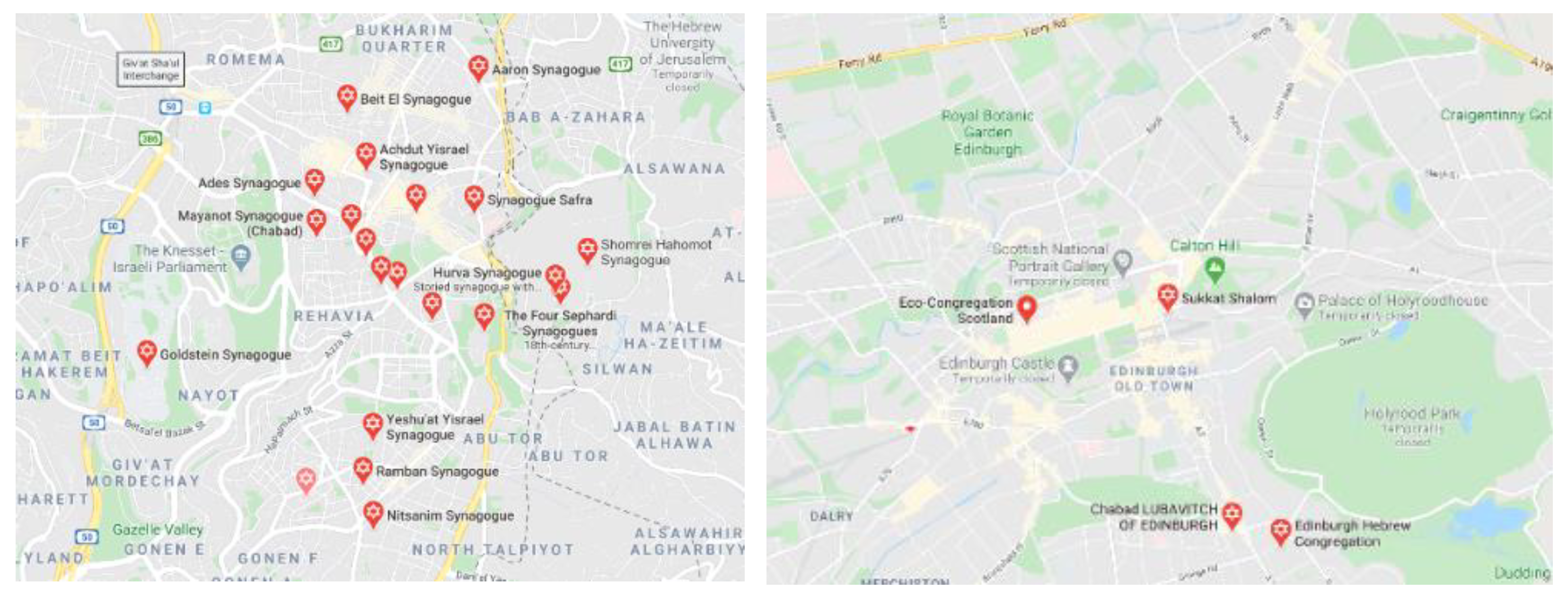
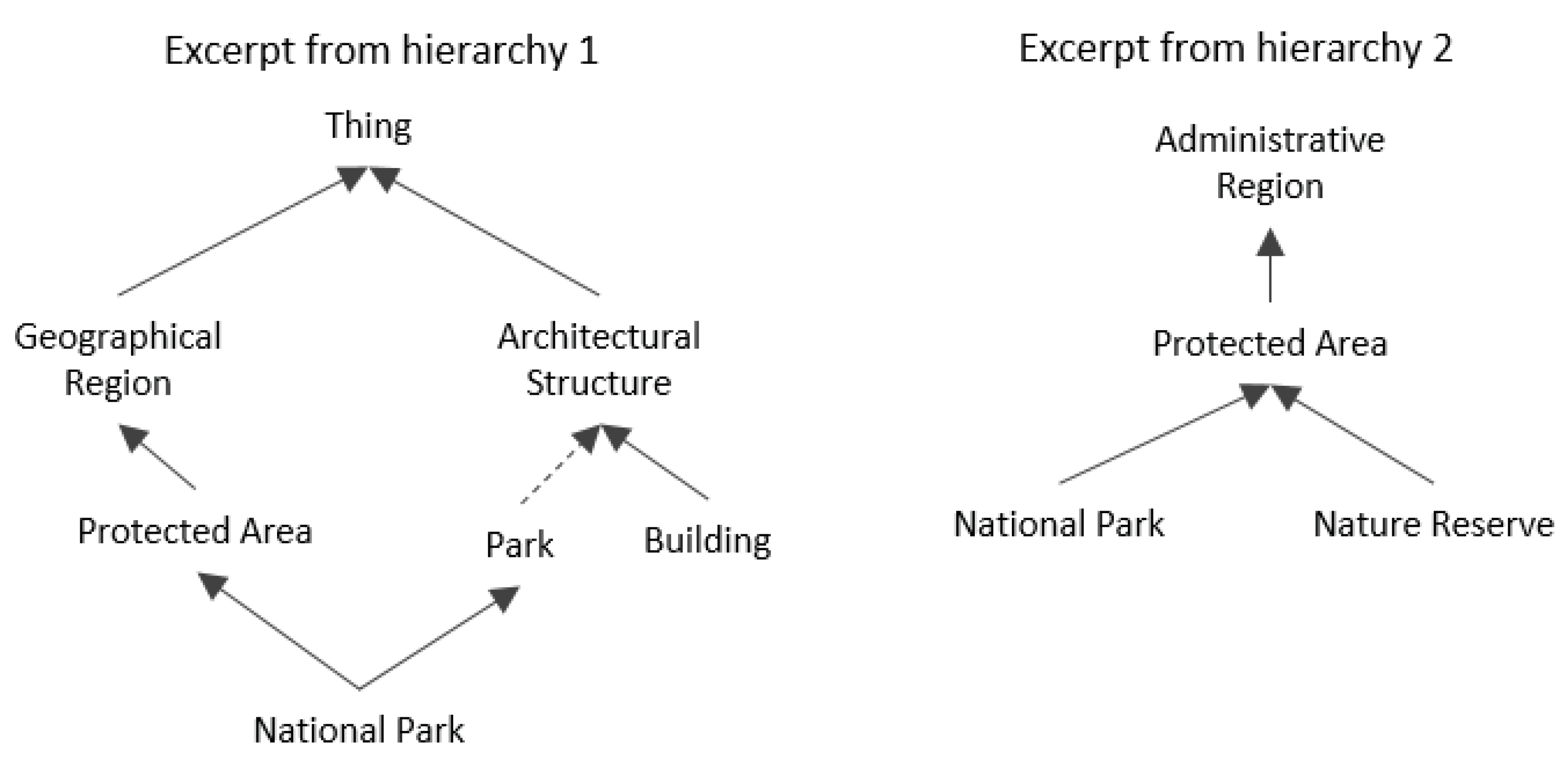
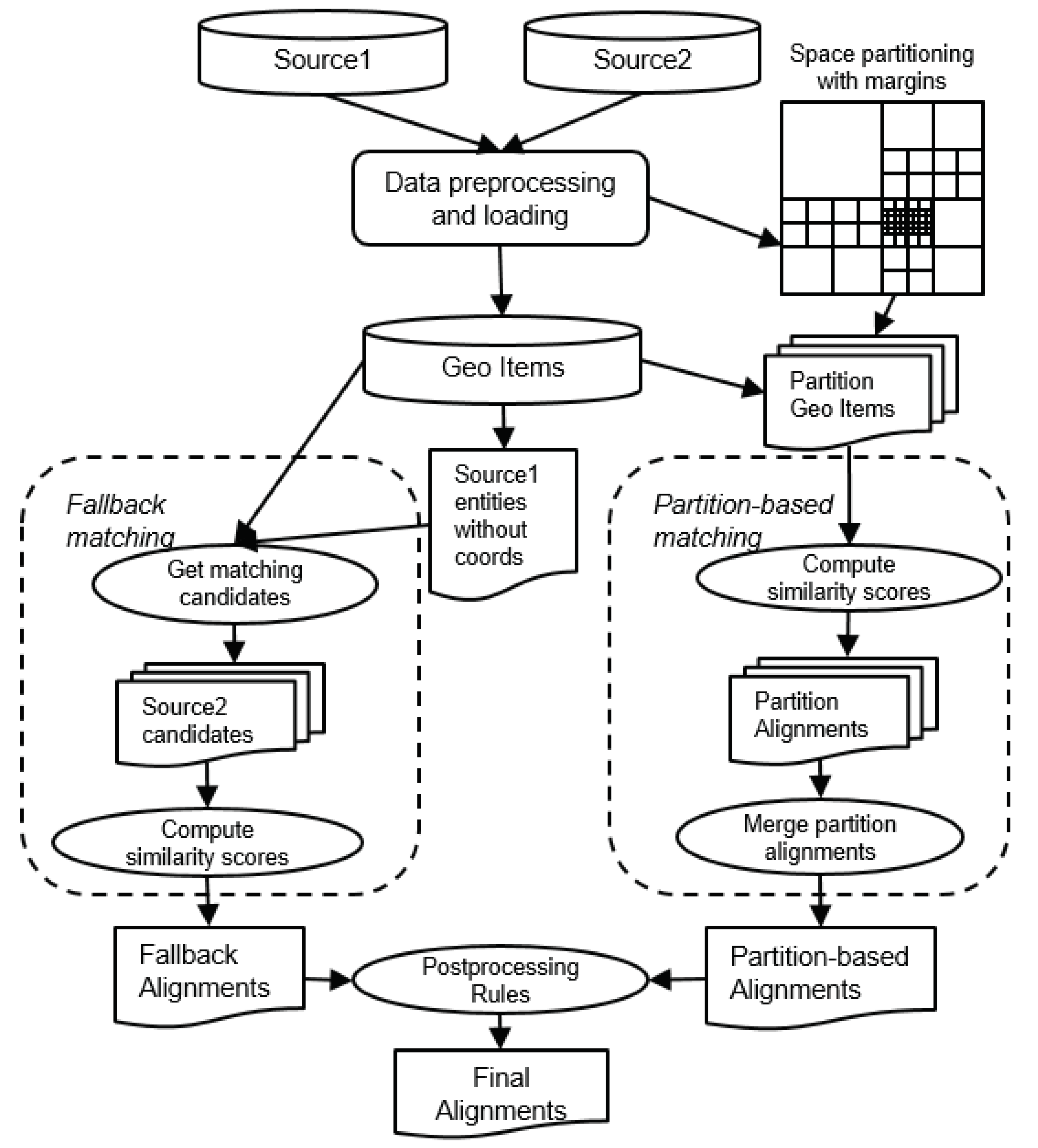
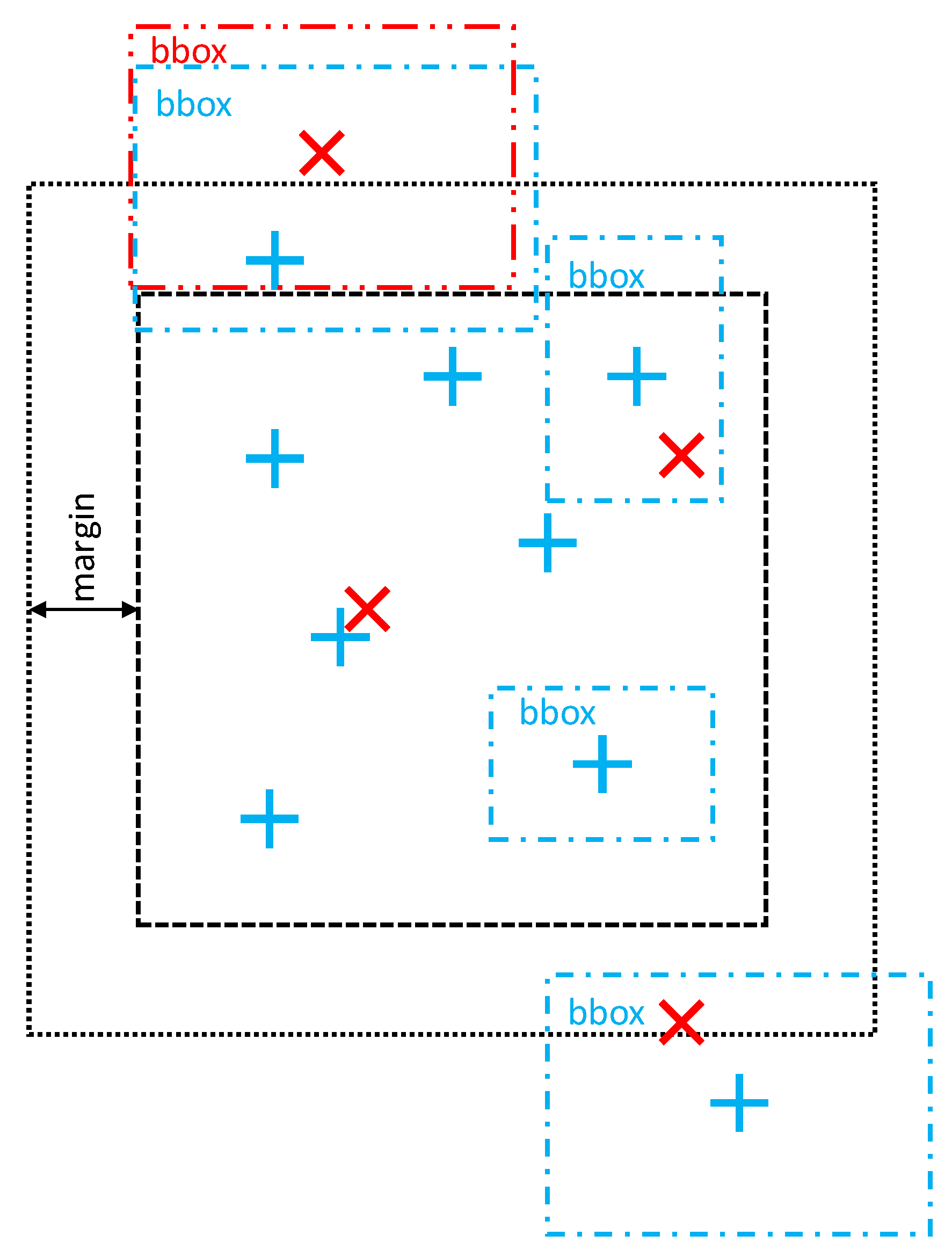
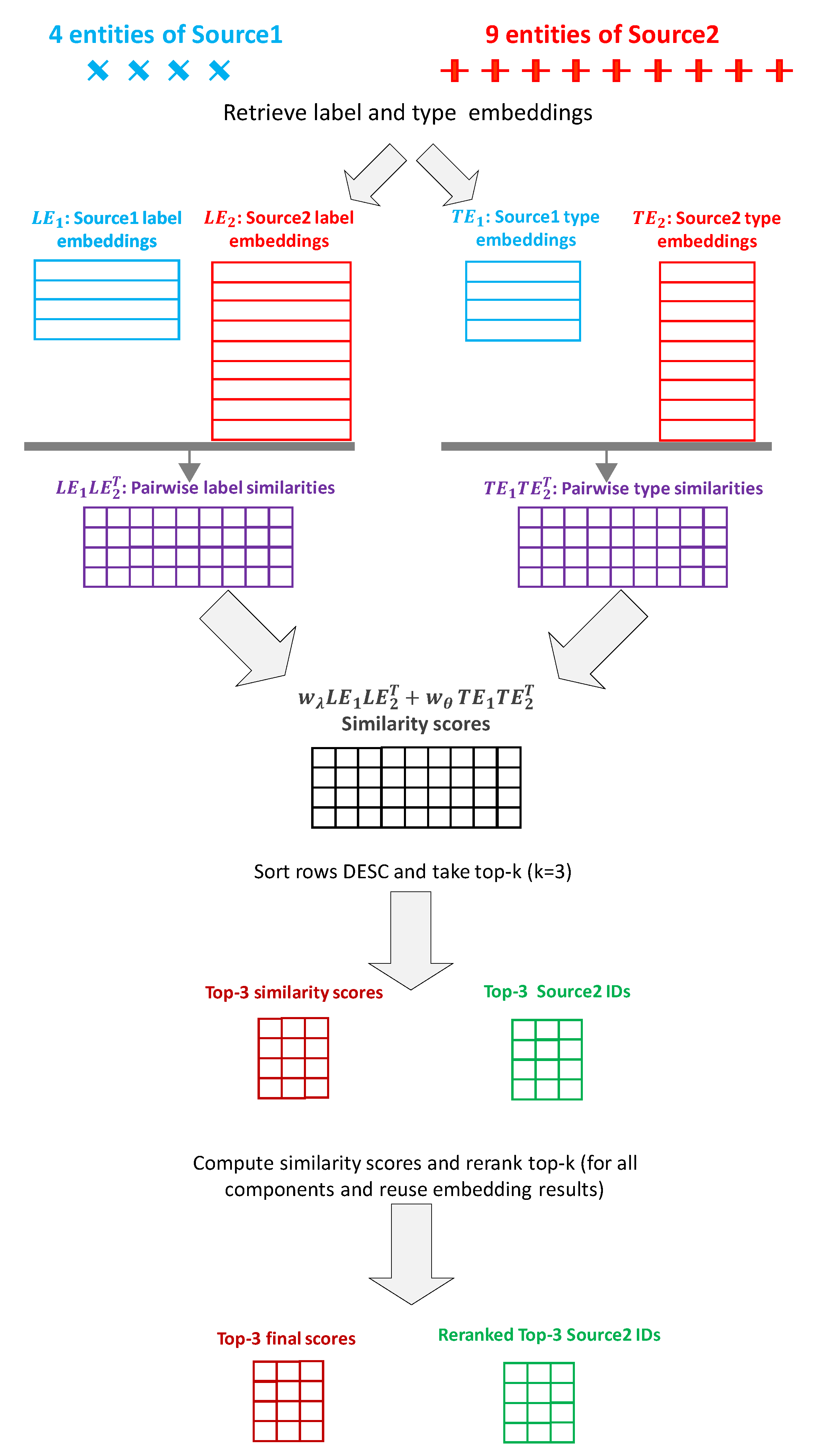
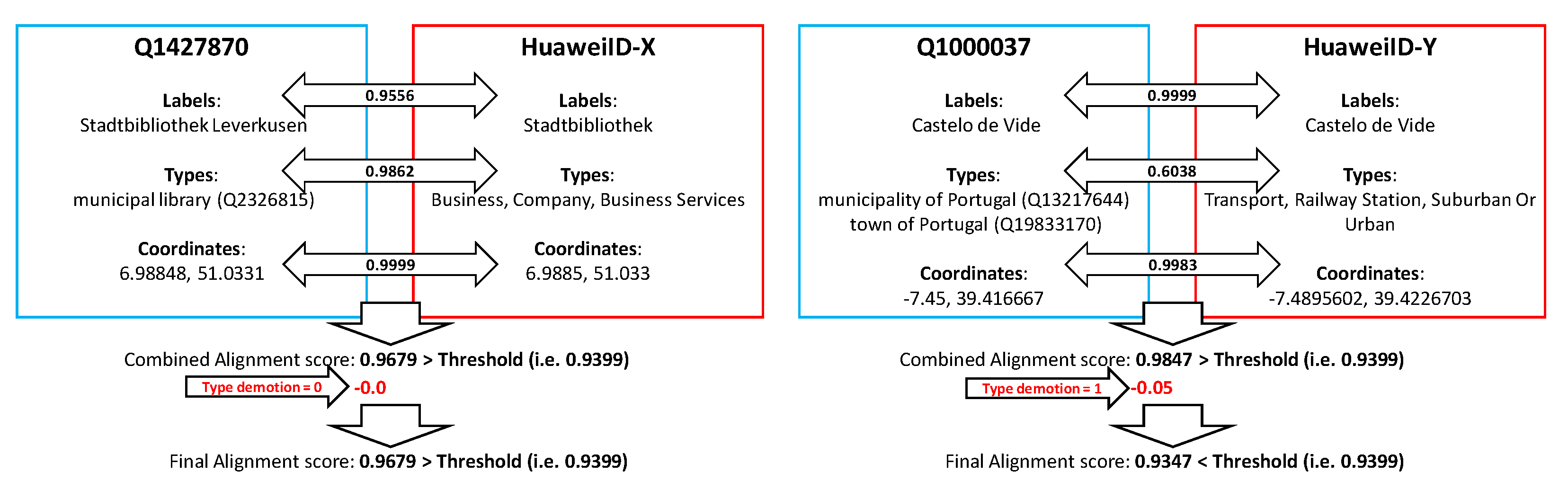
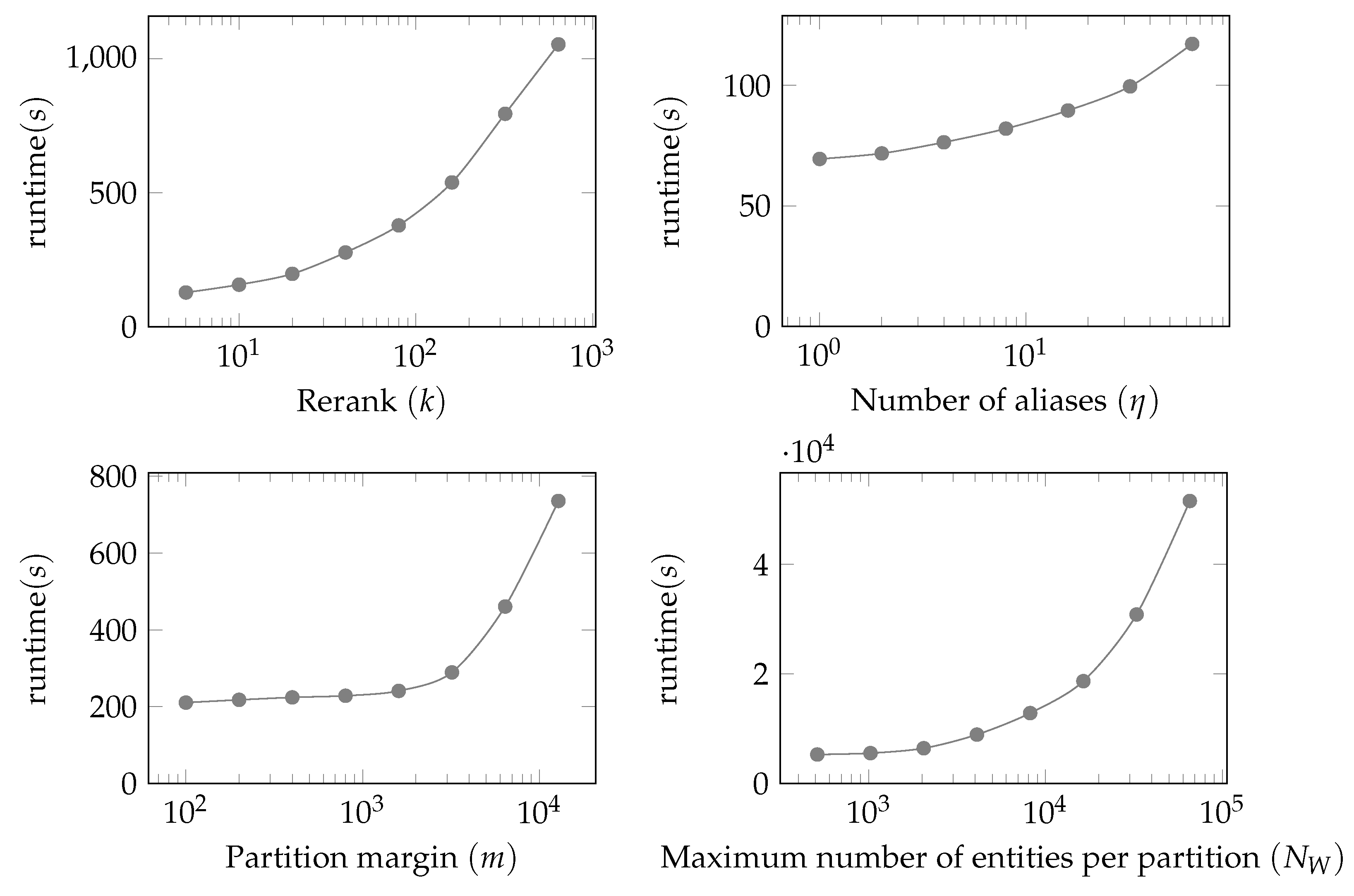
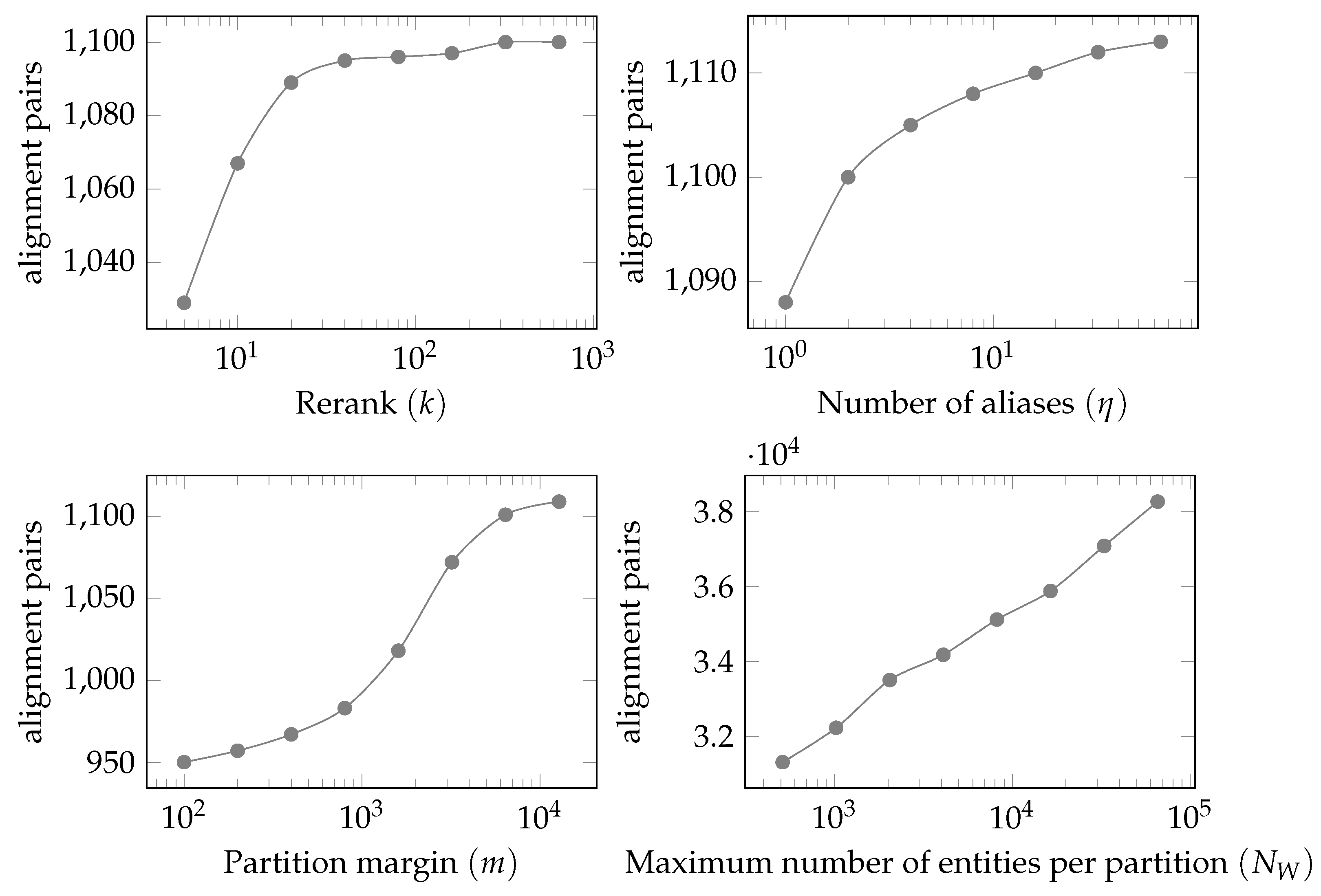
Table 1.
Dataset statistics.
| Dataset | HuaweiPD | Wikidata |
|---|---|---|
| Entities | 105.5 M | 8.1 M |
| Coordinates | 105.5 M | 7.7 M |
| BoundingBoxes | 1.1 M | 8.8 K |
| Labels/Aliases | 114.6 M | 37.1 M |
| Languages | 237 | 441 |
| Types | 744 | 2.4 M |
| SubClassOf | 731 | 2.9 M |
Table 2.
Ablation experiment results.
| Ablated | F1-Score | Precision | Recall | Accuracy |
|---|---|---|---|---|
| GLEAN | 0.913 | 0.973 | 0.860 | 0.953 |
| LIDFJ | 0.888 | 0.984 | 0.810 | 0.940 |
| MLSE | 0.792 | 0.973 | 0.668 | 0.897 |
| TypeComp | 0.886 | 0.936 | 0.842 | 0.943 |
| TypeDem | 0.820 | 0.894 | 0.757 | 0.907 |
| TypeGD | 0.857 | 0.949 | 0.781 | 0.928 |
Publisher’s Note: MDPI stays neutral with regard to jurisdictional claims in published maps and institutional affiliations. |
© 2022 by the authors. Licensee MDPI, Basel, Switzerland. This article is an open access article distributed under the terms and conditions of the Creative Commons Attribution (CC BY) license (https://creativecommons.org/licenses/by/4.0/).
Share and Cite
MDPI and ACS Style
Melo, A.; Er-Rahmadi, B.; Pan, J.Z. A System for Aligning Geographical Entities from Large Heterogeneous Sources. ISPRS Int. J. Geo-Inf. 2022, 11, 96. https://0-doi-org.brum.beds.ac.uk/10.3390/ijgi11020096
AMA Style
Melo A, Er-Rahmadi B, Pan JZ. A System for Aligning Geographical Entities from Large Heterogeneous Sources. ISPRS International Journal of Geo-Information. 2022; 11(2):96. https://0-doi-org.brum.beds.ac.uk/10.3390/ijgi11020096
Chicago/Turabian StyleMelo, André, Btissam Er-Rahmadi, and Jeff Z. Pan. 2022. "A System for Aligning Geographical Entities from Large Heterogeneous Sources" ISPRS International Journal of Geo-Information 11, no. 2: 96. https://0-doi-org.brum.beds.ac.uk/10.3390/ijgi11020096
Note that from the first issue of 2016, this journal uses article numbers instead of page numbers. See further details here.