
Crop Identification Based on Multi-Temporal Active and Passive Remote Sensing Images

School of Surveying and Land Information Engineering, Henan Polytechnic University, Jiaozuo 454000, China
*
Author to whom correspondence should be addressed.
ISPRS Int. J. Geo-Inf. 2022, 11(7), 388; https://0-doi-org.brum.beds.ac.uk/10.3390/ijgi11070388
Submission received: 17 April 2022
/
Revised: 4 July 2022
/
Accepted: 8 July 2022
/
Published: 11 July 2022
(This article belongs to the Special Issue Integrating GIS and Remote Sensing in Soil Mapping and Modeling)
Abstract
:Although vegetation index time series from optical images are widely used for crop mapping, it remains difficult to obtain sufficient time-series data because of satellite revisit time and weather in some areas. To address this situation, this paper considered Wen County, Henan Province, Central China as the research area and fused multi-source features such as backscatter coefficient, vegetation index, and time series based on Sentinel-1 and -2 data to identify crops. Through comparative experiments, this paper studied the feasibility of identifying crops with multi-temporal data and fused data. The results showed that the accuracy of multi-temporal Sentinel-2 data increased by 9.2% compared with single-temporal Sentinel-2 data, and the accuracy of multi-temporal fusion data improved by 17.1% and 2.9%, respectively, compared with multi-temporal Sentinel-1 and Sentinel-2 data. Multi-temporal data well-characterizes the phenological stages of crop growth, thereby improving the classification accuracy. The fusion of Sentinel-1 synthetic aperture radar data and Sentinel-2 optical data provide sufficient time-series data for crop identification. This research can provide a reference for crop recognition in precision agriculture.
1. Introduction
As the world’s population continues to grow and the COVID-19 pandemic brings uncertainties, food security has gained increasing attention [1,2,3]. At the same time, driven by the digital revolution in agriculture, two major changes have taken place in world agriculture: the development of precision agriculture, and the development of the agricultural digital economy [4,5,6]. Integrating GIS and remote sensing to obtain and analyze crop planting information is the key to realizing intelligent agriculture [7]. Remote sensing, with its rapidity, accuracy, and numerous other advantages, is now widely used to extract and classify crops, which is vital for intelligent agriculture [8].
Multi-temporal passive remote sensing plays an important role in agriculture [9]. Since the growth of crops follows seasonal rhythms and regular phenological variations, a time series of multi-temporal remote-sensing data can characterize crops as a function of time [10,11,12]. Sonobe et al. (2017) used data from the Landsat 8 Operational Land Imager to classify crops in Hokkaido, Japan and achieved an overall accuracy of 94.5% [13]. Yi et al. (2019) extracted various features from multi-temporal Sentinel-2 data for crop classification and obtained an overall accuracy of 94% [14].
The above Landsat 8 and Sentinel-2 optical data were obtained by passive remote sensing platforms [15]. Sentinel-2 is a multispectral high-resolution imaging satellite that carries a Multispectral Instrument (MSI) [16]. It has two satellites 2A and 2B, and each satellite conducts an Earth observation every 10 days under constant-observation conditions [16]. The complementarity of the two satellites can achieve a temporal resolution of 5 days. The MSI has 13 bands that cover from 442 to 2202 nm, and the highest spatial resolution is 10 m [16]. With its three bands in the red edge, Sentinel-2 can provide rich information for crop detection and thereby greatly improve the estimation accuracy for chlorophyll content, the fractional cover of forest canopies, and leaf area index [17]. In addition, Sentinel-2 data have high temporal resolution, so their use can provide rich temporal information for short-term crop identification over large areas [18]. Although the vegetation indices (VIs) feature of optical images provides an efficient method for crop identification, they are easily affected by cloud cover and are difficult to obtain as complete time series [19].
Since microwaves can penetrate clouds, active remote sensing can be done independently of weather conditions, which greatly facilitates the acquisition of continuous time-series images [20]. Sentinel-1 is a radar satellite launched by the European Space Agency with high spatial resolution and a short revisit period. It has four working modes: wave (WV), interferometric wide swath (IW), extra-wide swath (EW), and stripmap (SM) [21], and can provide single-polarized (HH or VV), dual-polarized (HH + HV or VV + VH), multi-temporal, high-resolution (down to 5 m), and C-band synthetic aperture radar (SAR) imaging data. Researchers have already applied Sentinel-1 data to crop identification [22,23,24,25]. Teja et al. used Sentinel-1 temporal SAR data to estimate Kharif rice planting areas and obtained an overall accuracy of 91% [25]. To better identify crops, many scholars used both Sentinel-1 and -2 data [26,27,28]. However, few studies have focused on feature-level fusion, which is helpful for dealing with information redundancy [29].
The random forest (RF) classifier can classify fused remote sensing data [30]. RF is an ensemble learning method used to solve classification and regression problems [31]. Ensemble learning is a machine learning scheme that improves prediction accuracy by integrating multiple models to solve a given problem [32]. Multiple classifiers participating in ensemble classification produce more accurate results than a single classifier [32]. In addition, RF can extract multisource features through multiple decision trees, thus making the most of the features used in fused data. In particular, for time-series features, RF uses the statistical characteristics of time-series data to extract and analyze the time-series features of different samples [33]. Finally, due to the simple and efficient decision-making method of majority voting, RF classifiers can quickly classify large quantities of remote-sensing data [34].
This paper focuses on the autumn crops in Wen County, Jiaozuo City. Using multi-temporal Sentinel-1 and -2 data, this study fused the backscattering coefficient of Sentinel-1 and the normalized difference vegetation index (NDVI) of Sentinel-2 data at the feature-level, then used a GIS platform to make samples, and finally used RF for classification. The classification results of fused data, single-temporal Sentinel-2 data, multi-temporal Sentinel-1 data, and multi-temporal Sentinel-2 data were compared to elucidate the advantages of multi-temporal data and fused data for crop identification.
2. Materials and Methods
2.1. Study Area
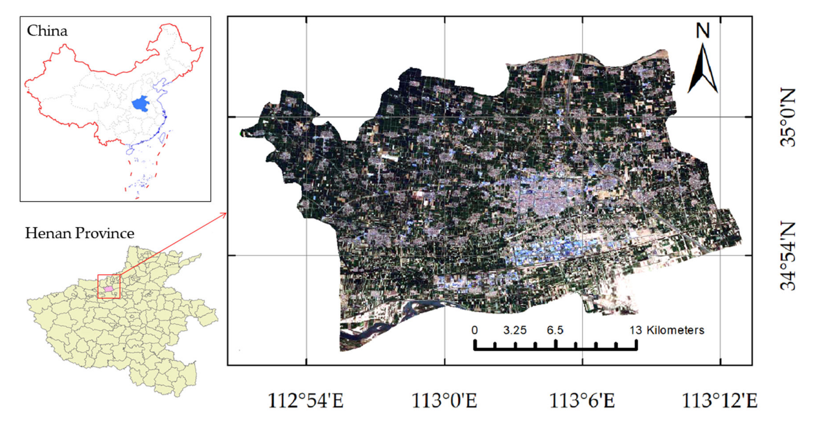
Wen County, Jiaozuo City is situated in northwest Henan Province, China (112°57′39″–113°02′43″ E, 34°50′15″–34°57′37″ N) and has a warm temperate continental monsoon climate. The average temperature is between 14 and 15 °C, and the annual rainfall is between 550 and 700 mm. Most of Wen County is plain, and the average elevation (relative to the average sea level) is between 102.3 and 116.1 m. The multiple historical floodings of the Yellow River and the Qin River formed the unique landforms of the south beach, the north depression, and the middle hill in Wen County. The inland rivers belong to the Yellow River system. The Yellow River, Qin River, and the drainage river system flow through the area, providing sufficient water resources and convenient irrigation. The main types of soil in this area are yellow fluvo-aquic soil and cinnamon fluvo-aquic soil, and long-term farming gives this area significant production potential. This paper focuses mainly on the autumn crops in Wen County, mainly including corn, peanut, and Chinese yam, accounting for about 96% of the total crops. Other non-major crops, mainly including sweet potatoes, oil crops, vegetables and fruits, fall outside the scope of this paper. Figure 1 shows the geography of Wen County.
2.2. Sentinel-1, -2 Data
For this research, ground range detected (GRD) Sentinel-1 C-band (5.405 GHz) level-1 images in IW mode were downloaded from the website of ASF Data Search. IW mode supports the merging of wider strip widths (250 km), and the downloaded images have medium resolution (10 m). GRD products include two polarization modes, VV and VH. The range and azimuth resolutions are 20 and 22 m, respectively, and the pixel spacing is 10 m. Table 1 shows the data from Sentinel-1 imagery products.
This study uses multi-temporal Sentinel-2 data for crop identification. Table 2 lists the dates of Sentinel-2 image acquisition. These Level-2A data cover different plant growth periods from June 2020 to October 2020, and the data were obtained from the PIE (Pixel Information Expert) Engine platform.
2.3. Field Data
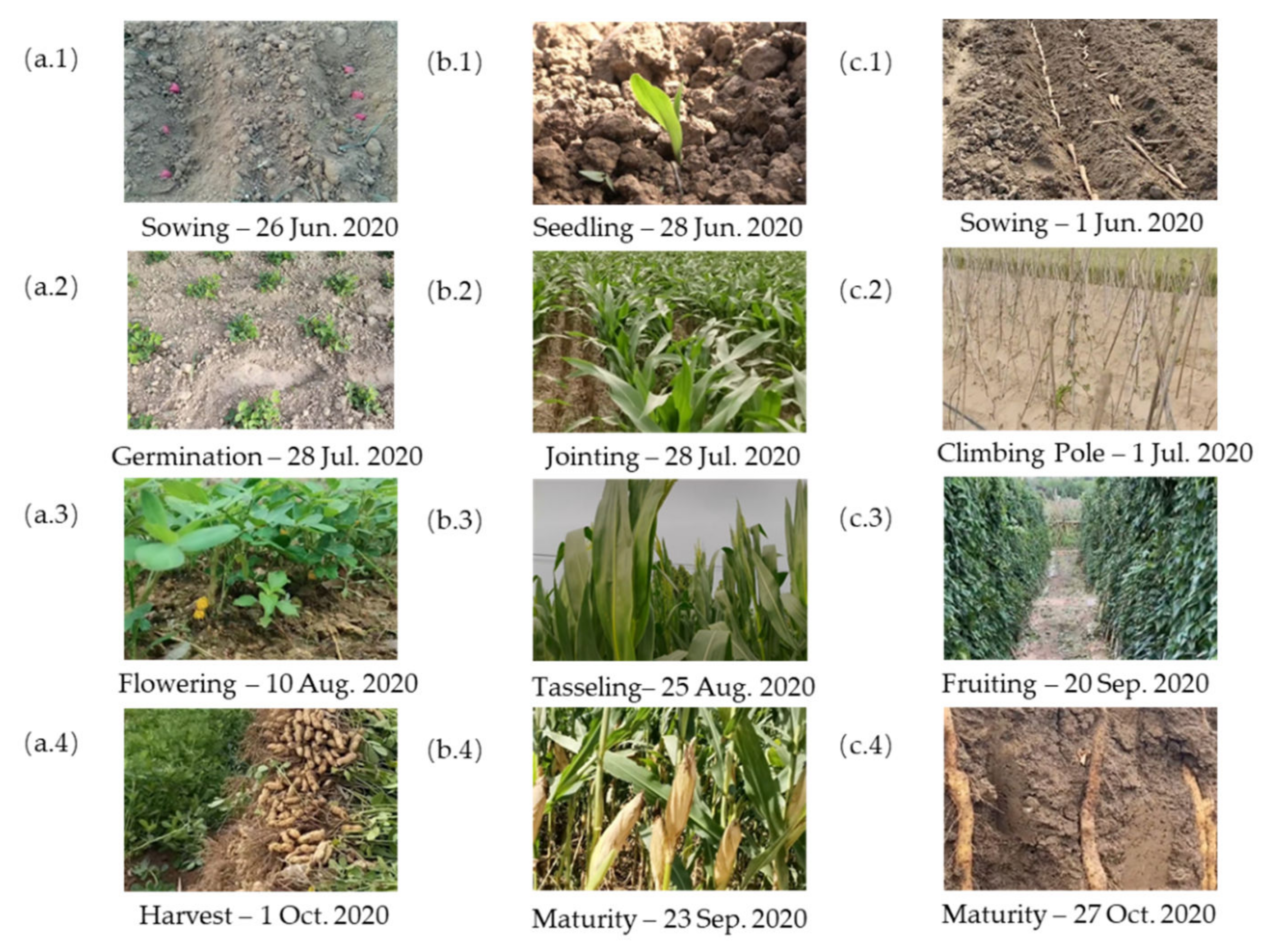
To understand the local crop-planting situation in Wen County and obtain the training set and testing set labels for crop classification, this study conducted field visits at three different sites in the study area in September 2020. This study consulted the local agricultural production departments and farmers in detail about the planting phenology of autumn crops. The statistical results are given in Table 3, and Figure 2 shows representative crop images.
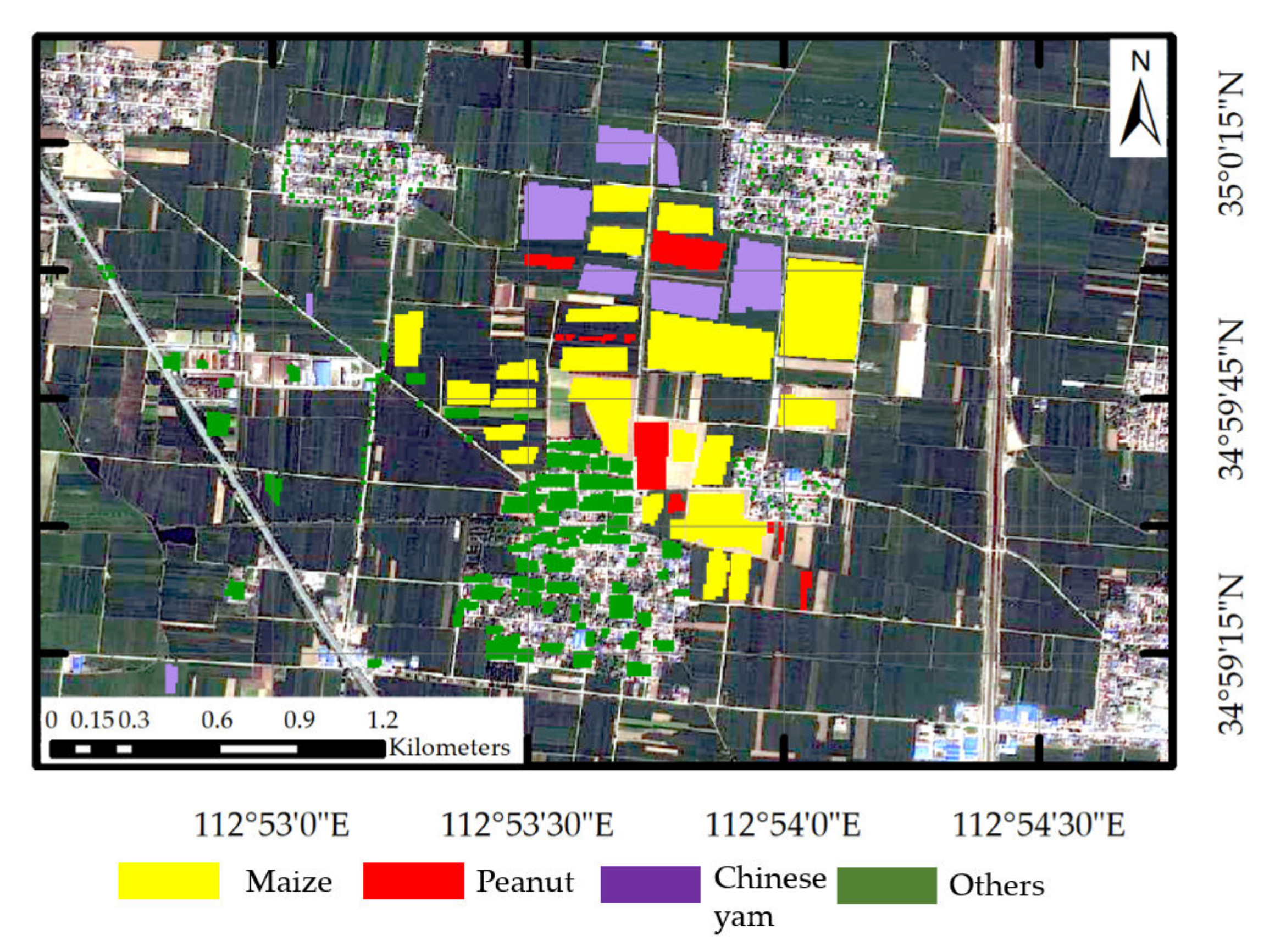
In the field visits, in addition to recording the crop attributes for each parcel, the center latitude and longitude coordinates of each parcel were recorded with a handheld differential GPS positioning tool using the WGS1984-UTM coordinate system (zone 49N), with less than 2 m positioning error. Using the ArcGIS10.6 (Esri, Redlands, CA, USA) software platform, the data generated by GPS positioning and attribute data were merged and converted into ESRI shapefile format and matched to Google’s high-resolution remote sensing images. This study used visual interpretation to label polygons on Google Image with the shapefile as the center. In terms of the ground sample distance of Sentinel-1 and -2 data, each polygon was at least 10 m from the boundary to avoid pixel mixing at the boundary. Some of the labels are shown in Figure 3. “Others” includes non-major crops, established areas, water, roads, and trees.
Table 4 lists the ratio of labeled area to corresponding crop area. The crop area data came from the 2020 Jiaozuo City Statistical Yearbook data.
2.4. Methods
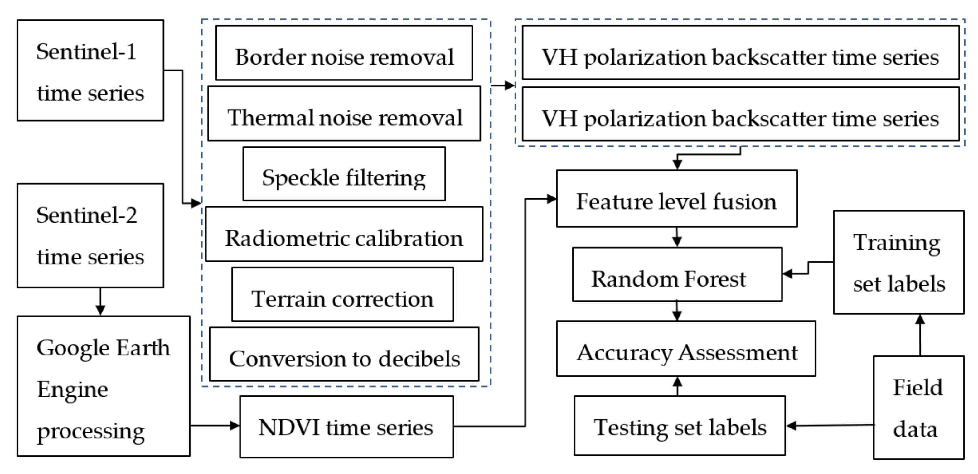
The research method used herein mainly focused on the fusion of Sentinel-1 and -2 data. This paper not only studied the role of multi-temporal data in crop identification but also discusses the advantages of fusing active and passive remote-sensing images for crop classification. Figure 4 shows a flowchart of the process.
2.4.1. Time-Series Datasets
Sentinel-1 was preprocessed using the open-source remote-sensing processing software SeNtinel Applications Platform (SNAP) of the European Space Agency and ENVI5.3 (Esri, Redlands, CA, USA). The main processes included removal of border noise and thermal noise, speckle filtering, radiometric calibration, terrain correction, conversion to decibels, and image clipping [35]. The time-series datasets with VV and VH polarization were obtained by preprocessing, which includes the backscattering coefficient. This study normalized features in both datasets: the pixel values of each image were transformed to a common scale, and the inherent similarities and variations were preserved. Feature normalization can improve the performance of machine learning algorithms. The normalization uses the min-max normalization type, with a minimum value of 2% and a maximum value of 98%, to reduce sensitivity to outlier.
Sentinel-2 data were preprocessed using PIE Engine, the optical features extracted, and a normalized difference vegetation index (NDVI) time-series dataset was constructed. Extracting the NDVI time-series features of Sentinel-2 is the key to studying crop mapping [14]. The NDVI correlates strongly with leaf area index and plant chlorophyll, and it is an important tool to study vegetation growth status and vegetation coverage and eliminate radiation errors [36]. Its time-series curve reflects the growth cycle of crops, including sowing, germination, heading, maturity, and harvest [37,38,39]. NDVI is calculated according to the normalized transformation of near-infrared and red reflectance, which is given by Equation (1).
where is the reflectance in the near-infrared band and is the reflectance in the red band.
To extract the study area, the vector boundaries of Wen County were read as feature classes in the PIE Engine and overlaid onto Sentinel-2 images. Then, this study performed operations such as cloud removal, NDVI band math, filtering, and batch exporting. In particular, the quality assessment band was used to detect clouds and cloud shadows for simple and efficient cloud detection and removal. To facilitate the calculations involved in machine learning, feature normalization was performed on the acquired NDVI time-series dataset.
2.4.2. Fusion of Active and Passive Remote Sensing
The fusion of different sensor data generally requires georeferencing and image fusion [40]. In this study, both active and passive remote sensing time-series datasets were projected to the WGS1984-UTM coordinate system (zone 49N), so georeferencing is not required before fusion.
Most of the fusion of optical and radar images adopts an early fusion strategy, in which the optical image time series and the radar image time series are stacked together in the form of a data cube [41,42,43,44]. This fusion method does not extract vegetation index and backscattering coefficient, so it is simple and easy to implement. However, the fusion data have too much information, most of which is not important for crop identification, so information redundancy is a problem [29]. Therefore, this study adopted here the feature-level fusion method, whereby this study selected the backscattering coefficient feature from Sentinel-1 and the VI feature from Sentinel-2, and obtained the fused data by stacking the corresponding time-series dataset. In more detail, the fusion data contain 9 NDVI, 10 VV polarization backscattering coefficients and 10 VH polarization backscattering coefficients.
2.4.3. Random Forest Classifier
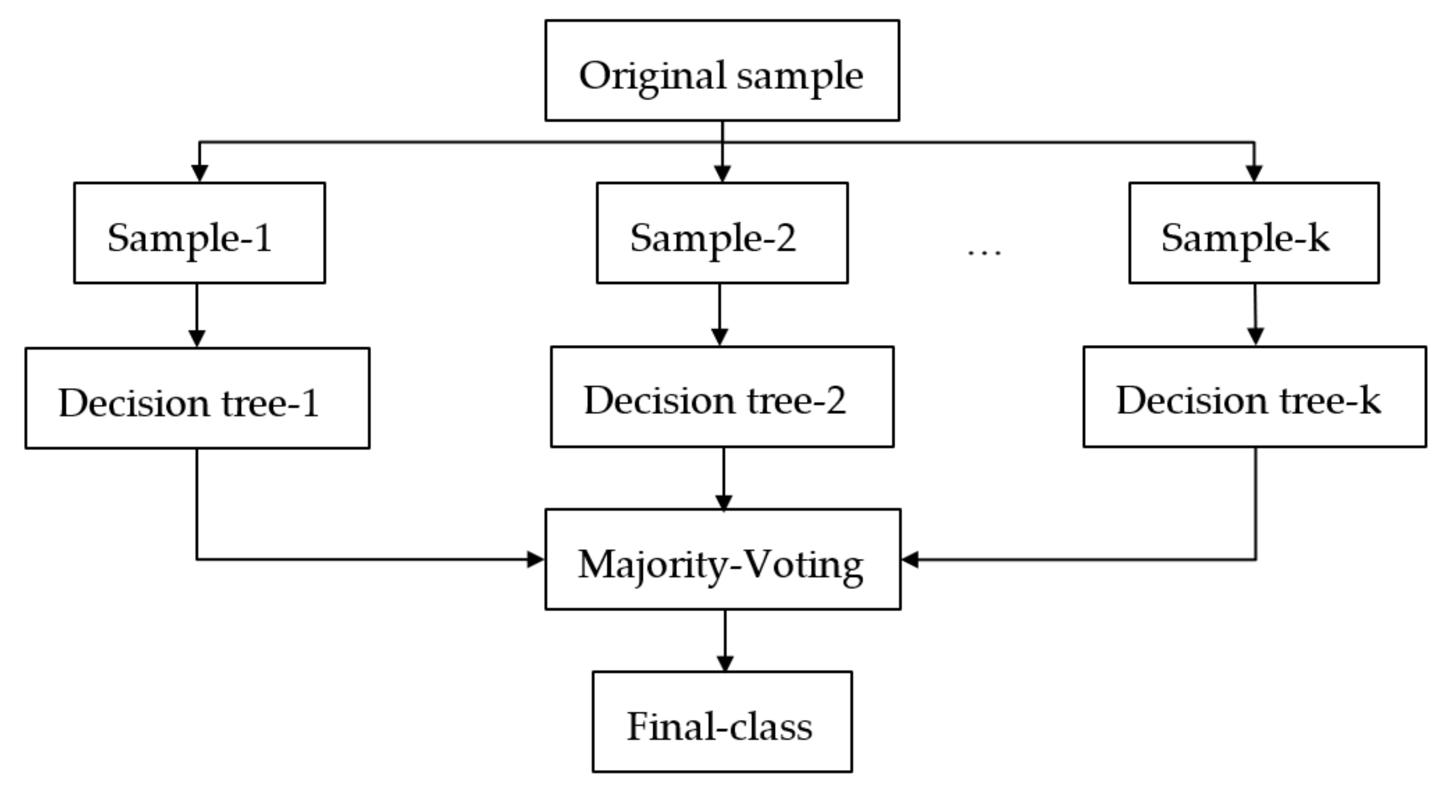
This study used a semantic segmentation algorithm based on the RF classifier to classify Sentinel-1 and -2 fused data. Unlike instance segmentation, which treats a single object as a distinct entity regardless of its category, semantic segmentation treats all objects of the same category as belonging to one entity [45,46]. Due to the complexity of remote-sensing image applications and the similar structure of crops, this study used a classification method of semantic segmentation. RF is a supervised machine learning algorithm that meets the needs of semantic segmentation [47]; it consists of multiple decision trees, and the category of each pixel of its output depends on the maximum number of votes in the set of trees. RF is faster than other classifiers, easier to parameterize, and robust [48], which supports the analysis of various features used herein. Figure 5 shows the structure of RF, and the RF classifier involved four main steps:
- (1)
- A sample set with capacity N was extracted N times with one-at-a-time replacement until N samples were formed, which were then used as the samples at the root node of the decision tree to train the decision tree;
- (2)
- Each sample has M features. When the decision tree needed to be split, m << M features were selected at random from these M features. The feature with the best classification ability of these m features was selected as the splitting feature of the node;
- (3)
- To form the decision tree, each node was split as per step 2 until the feature selected by the child node was the feature used when the parent node was split; that is, the child node was a leaf node. At this point, the splitting stopped. Note that each tree grew to the maximum extent, and no pruning was done during the formation of the decision tree; and
- (4)
- This study followed steps 1–3 to build k decision trees to form a RF. Assuming that the set of categories was {, , …, }, the prediction output of in sample x was expressed as an N-dimensional vector , where represented the output of in category , and the decision was made by the majority voting (Equation (2)).
That was, if a category got more than half of the votes, the prediction would be that category, otherwise the prediction would be rejected.
The RF classifier had two parameters to set: the number k of decision trees in the classifier and the number m of features to consider when finding the best split [49]. The more decision trees in the RF classifier, the better the classification, but the longer the calculation time; the smaller the number of features, the smaller the variance, although the bias would increase. Therefore, the classification accuracy and time efficiency were comprehensively considered. This study used 300 decision trees, and the root of the total number of features was taken as the number of features.
2.4.4. Training and Prediction
For classification training and testing, the sample labels were overlaid on the fused images to obtain the samples. To avoid the influence of spatial autocorrelation [50], samples from two sites in the study area were used as the training set, and the other samples were used as the testing set. Table 5 lists the number of pixels and parcels for the training set and the testing set.
The training set data were input into the parameterized RF classifier for training, and then the trained RF model was used to make predictions from the testing-set images. To evaluate the advantages of fused data and multi-temporal data, the time series of backscatter coefficients of Sentinel-1, the NDVI time series of Sentinel-2, and the NDVI images of single-temporal Sentinel-2 (on this day, all categories are easily distinguished) were also used to train the classifier and to make predictions with the same parameters.
2.4.5. Accuracy
Four schemes were used to evaluate the accuracy of the predictions. The most commonly used technique to assess the accuracy of crop classification involves the confusion matrix [51]. The confusion matrix compares the predicted images of the testing set with the labels of the testing set and produces the overall accuracy (OA%) and Kappa coefficient (K) (Equations (3) and (4)), which are the probability that the pixels are correctly classified and measure the consistency between the classification result and the actual result [48]. The OA was given by
where is the total number of pixels belonging to category i and assigned to category j and n is the number of categories. The Kappa coefficient was given by
where N is the total number of pixels,, , …, are the numbers of real pixels in each type, and , , …, are the numbers of pixels predicted for each type [52]. In addition, to fully verify the classification results obtained, this study compared the classification results of the fused data with the 2020 Jiaozuo City Statistical Yearbook data.
3. Results
3.1. Time Series Curve
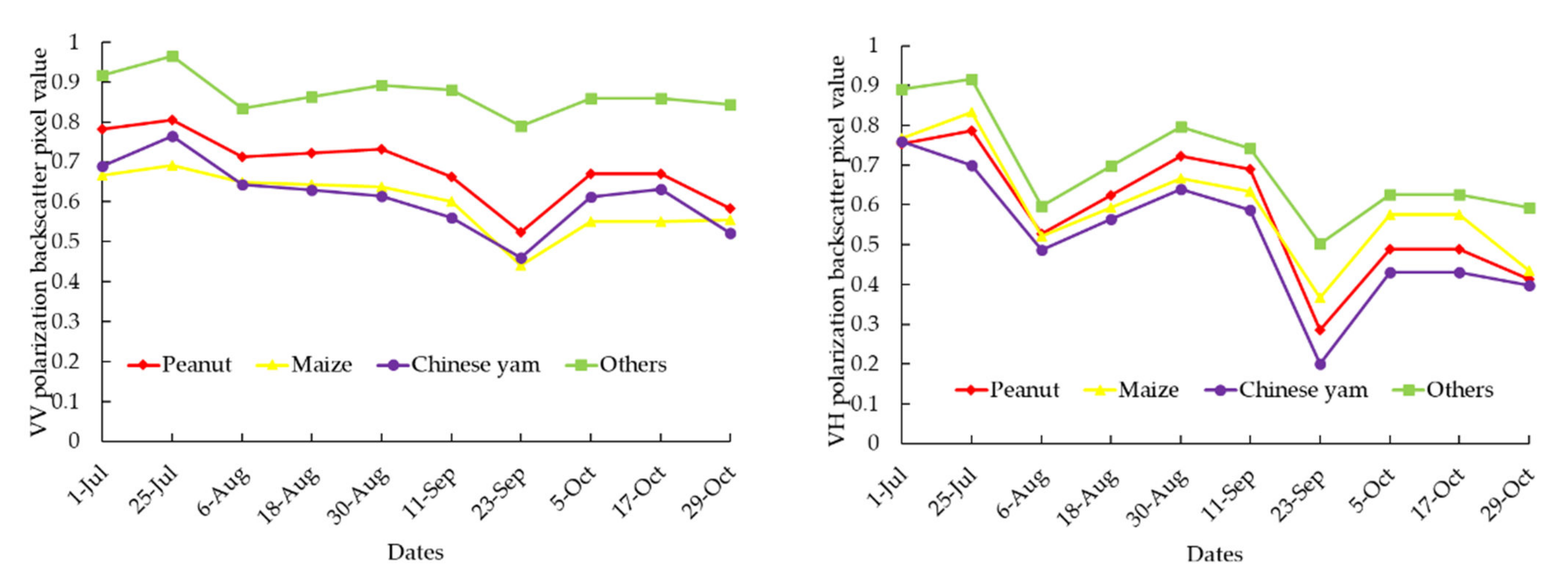
Figure 6 shows the time-varying curves of VV and VH polarization backscatter coefficients for different categories after feature normalization. The pixel value of this backscatter coefficient is the average value of each class sample. It can be seen from Figure 6 that the pixel values changed with time; the pixel values of VV changed little, while the pixel values of VH changed greatly.
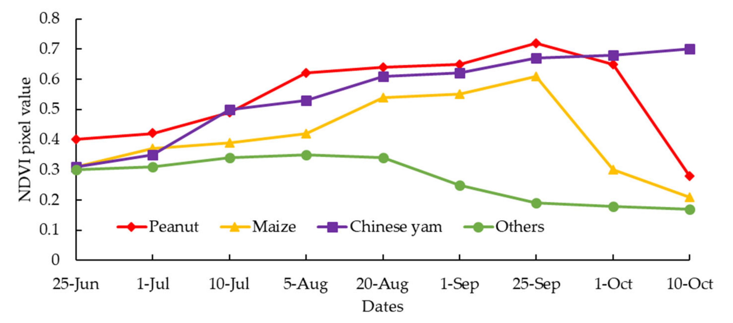
Figure 7 shows the NDVI pixel values after feature normalization and as a function of time for different categories. The NDVI pixel value is the average of the NDVI pixel values for all samples in that category. The results showed that the NDVI value of crops changed with time, which was consistent with the growth process of crops [11]. On August 5, the categories were easy to distinguished, so this study selected the Sentinel-2 data on this day as the single-temporal data.
3.2. Accuracy
The OAs and Kappa coefficients are given in Table 6. Compared with the 5 August 2020 Sentinel-2 data, the OA of the multi-temporal Sentinel-2 data increased by 6.3%, and the Kappa coefficient increased by 0.047. The fused multi-temporal Sentinel-1 and -2 data achieved the highest OA of 90.5% compared with multi-temporal Sentinel-2 (87.6%), 5 August 2020 Sentinel-2 (81.3%), and multi-temporal Sentinel-1 (73.4%).
For further comparison, the confusion matrix of the fused data is shown in Table 7. Maize achieved the highest producer’s accuracy at 91.5%, followed by other land cover (89.6%), yams (88.6%), and peanuts (85.2%). In terms of user’s accuracy, maize obtained the highest accuracy (96.4%), followed by other land cover (81.4%), peanuts (79.5%), and yams (75.1%).
3.3. Comparison of Details of Prediction
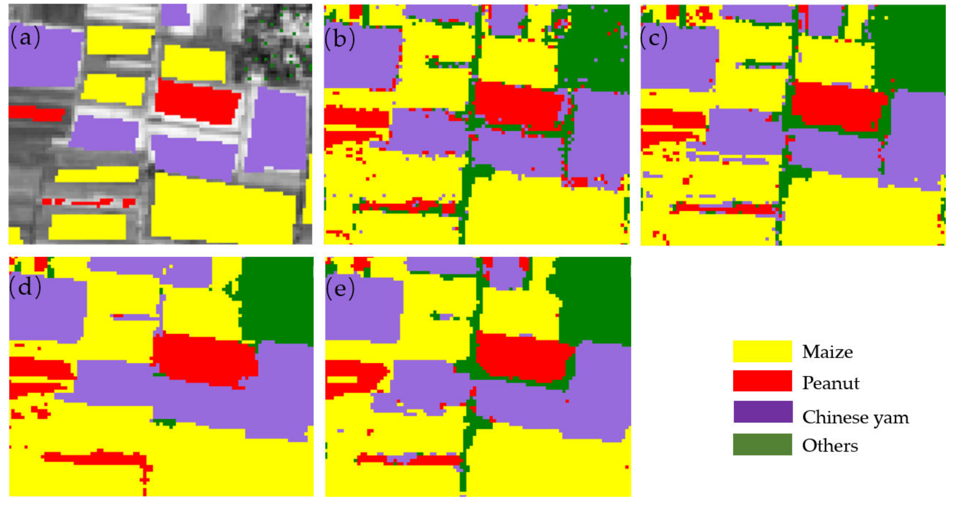
Figure 8 visually compares different predictions and testing set labels. On the one hand, multi-temporal Sentinel-2 data produced less image noise than single-temporal Sentinel-2 data and greater internal uniformity of the parcels. On the other hand, the fusion of multi-temporal Sentinel-1 and -2 data reduced the image noise of multi-temporal Sentinel-2 data and improves the prediction accuracy of multi-temporal Sentinel-1 data. With multi-temporal Sentinel-1 data, the edges of autumn crop parcels are the main areas of poor prediction, with minor linear objects, such as paths and streams, being incorrectly predicted as autumn crops.
3.4. Crop Mapping
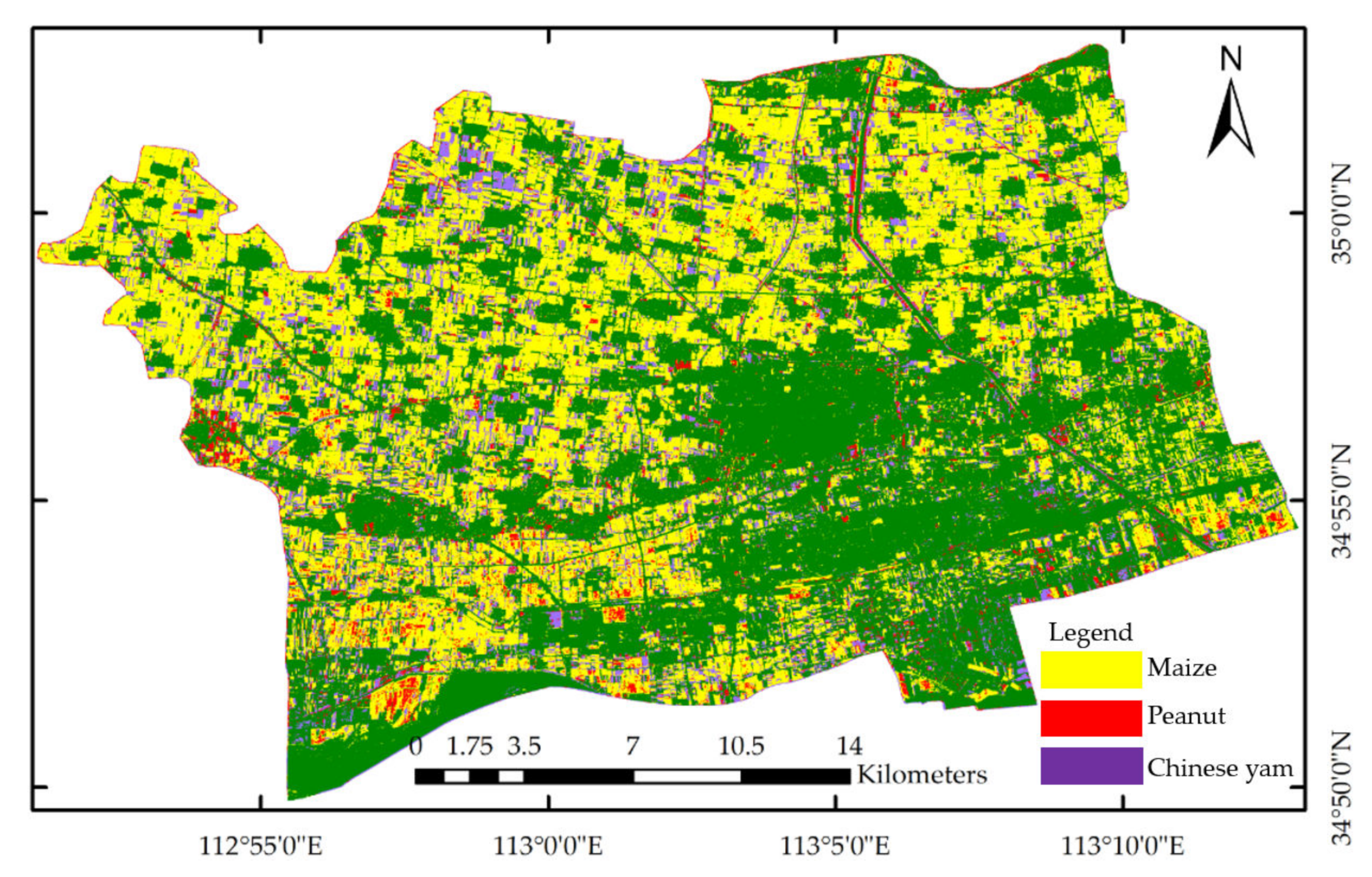
Figure 9 shows the spatial distribution of autumn crops in the study area, as determined by the fusion of multi-temporal Sentinel-1 and -2 data. From a spatial point of view, peanut, maize, and Chinese yam are mainly distributed in areas outside the southeastern part of Wen County. In terms of area, maize covers the largest fraction of crop area (74.95%), followed by Chinese yam (15.27%) and peanut (9.48%).
3.5. Comparison with Government Data
As shown in Table 8, the areas of peanut, maize, and Chinese yam reported by the government are all within the range predicted herein based on the fused data. Therefore, the classification results obtained herein correlate significantly with the 2020 Jiaozuo Statistical Yearbook data.
4. Discussion of Results
This study focuses on crop classification based on multi-temporal remote sensing data. The results showed that the use of the multi-temporal Sentinel-2 data significantly improved the classification accuracy. This result is attributed to the fact that crops have certain similarities during growth due to their physicochemical properties such as moisture and chlorophyll content and thereby have highly similar spectral characteristics [53]. This means that different crops may have the same spectral characteristics. The use of multi-temporal remote sensing imagery is thus crucial to clarify these ambiguities.
The time series of multi-temporal remote-sensing data characterized crops on a temporal basis, which provided a broader basis for identifying crop types, as demonstrated by the following four points: (1) The temporal dimension provided by the time-series data thus resolved the problem of the different crops having the same spectral characteristics or different spectral characteristics corresponding to the same crop, thus allowing the accurate, time-resolved determination of crops characteristics [54]. (2) Crop identification based on time-series data is not limited by seasons or crop phenology. By reconstructing or decomposing time-series curves, the effects of crop phenological changes in different periods can be eliminated and more general growth characteristics of crops can be explored, thereby eliminating the spurious variations caused by seasonal factors [55]. (3) The variations detected based on time-series data reflected multi-year changes in crops [56], which allows people to analyze how crops evolve over time. (4) The high temporal resolution of the time-series data allowed the accurate extraction of the temporal variations in crops.
The results show that the Sentinel-2 data lead to much greater accuracy than the Sentinel-1 data [57,58]. The NDVI of Sentinel-2 is an important index for crop area inversion and is widely used to extract crops and other vegetation [14,36]. For Sentinel-1 data, crops can only be extracted according to the change of backscattering coefficient, which is difficult to detect and distinguish crops.
The fusion of Sentinel-1 and -2 data is the key to this study. The results show that, compared with other data, the fused Sentinel-1 and -2 data provided the highest classification accuracy. This study used a feature-level fusion method to construct a multi-source remote-sensing fusion model that integrates multi-source features such as spectrum, time series, and backscatter coefficient. On the one hand, the combination of Sentinel-1 and -2 data provided more features for identifying crops. On the other hand, SAR data has strong anti-interference ability and is not affected by cloud cover. It can be acquired during the day or night under different weather conditions. Using Sentinel-1 data to supplement Sentinel-2 data solves the problem of cloud cover and insufficient time series data.
Some identification errors occurred in this study. A comparison of the classification details revealed that the pixels that should be classified as peanuts are instead classified as Chinese yams, and vice versa. Considering the growth phenology and vegetation indexes of the two crops, it can be found that their growth states are similar, which explains why it is difficult to distinguish Chinese yam from peanuts using remote sensing. However, the classification of maize is better because the phenology and VIs of maize differ from those of other crops. In addition, maize covers a large area so the samples are abundant, which is conducive to training an RF classifier.
The crop classification map and government data show the distribution of crops in Wen County. Maize is most widely distributed, much more so than Chinese yam or peanuts, because maize is the main food crop and has strong market demand, whereas peanuts and Chinese yam are local-specialty cash crops with small market demand. Wen is a typical agricultural county in China, so the good classification obtained in this work means that the method proposed herein can be transferred to other regions of China.
Future research should consider the following three aspects: (1) In feature selection, the multi-source remote sensing fusion model should be studied by integrating the spectral band, spectral index, texture feature, spectral index variation, and their combinations. (2) A variety of machine learning algorithms can be tested in comparative research. (3) Finally, to improve classification accuracy, multi-source remote-sensing fused data can be further enriched by, for example, airborne hyperspectral data, point cloud data, elevation data, and high-resolution data.
5. Conclusions
Given the population growth of recent decades, the rational use of land resources for crop planting has gained importance, and remote sensing provides an effective method to monitor crops. Radar satellites can be used to monitor the Earth’s surface on cloudy and rainy days, and optical data can be used to obtain vegetation indices to monitor crops. Therefore, compared with traditional remote-sensing data, the combination of radar and optical data can improve the accuracy with which crops are classified. The multi-sensor developed by the Copernicus program offers the fusion of data to improve crop identification. In this study, multi-source features such as backscatter coefficient, VIs, and time series were extracted from Sentinel-1 and Sentinel-2 data, and these features were fused at the feature-level. By using a RF classifier, this study obtained a Kappa coefficient of 0.881 and an overall accuracy of 90.5%, which shows that the fusion of multi-temporal active and passive remote sensing data can improve the accuracy of crop classification.
Author Contributions
Conceptualization, Hebing Zhang and Hongyi Yuan; methodology, Hongyi Yuan; software, Hongyi Yuan; validation, Hongyi Yuan, Hebing Zhang, Xiaoxuan Lyu and Weibing Du; formal analysis, Hongyi Yuan; investigation, Hebing Zhang; resources, Hongyi Yuan; data curation, Hongyi Yuan; writing—original draft preparation, Hongyi Yuan; writing—review and editing, Hebing Zhang, Hongyi Yuan, Xiaoxuan Lyu and Weibing Du; visualization, Hongyi Yuan; supervision, Hebing Zhang; project administration, Hebing Zhang; funding acquisition, Hebing Zhang. All authors have read and agreed to the published version of the manuscript.
Funding
This research was funded by the National Natural Science Foundation of China (grant number U21A20108), the Ministry of Education Cooperation in Production and Education (grant number 202102245019), the Joint Fund of Collaborative Innovation Center of Geo-Information Technology for Smart Central Plains, Henan Province and Key Laboratory of Spatiotemporal Perception and Intelligent processing, Ministry of Natural Resources (grant number No.211102), the PI project of Collaborative Innovation Center of Geo-Information Technology for Smart Central Plains, Henan Province (grant number 2020C002), the Doctoral Fund of Henan Polytechnic University(grant number B2022-8), the Fundamental Research Funds for the Universities of Henan Province(grant number NSFRF220424) and the project of Provincial Key Technologies R & D Program of Henan (grant number 222102320306).
Institutional Review Board Statement
Not applicable.
Informed Consent Statement
Not applicable.
Data Availability Statement
Not applicable.
Acknowledgments
We thank Piesat Information Technology Co., Ltd. for providing classification codes and related remote sensing data (website: https://www.piesat.cn/, accessed on 16 April 2022).
Conflicts of Interest
The authors declare no conflict of interest.
References
- Ayanlade, A.; Radeny, M. COVID-19 and food security in Sub-Saharan Africa: Implications of lockdown during agricultural planting seasons. NPJ Sci. Food 2020, 4, 13. [Google Scholar] [CrossRef] [PubMed]
- Stark, J.C. Food production, human health and planet health amid COVID-19. Explor.-J. Sci. Health 2021, 17, 179–180. [Google Scholar] [CrossRef] [PubMed]
- Wang, Y.; Peng, D.; Yu, L.; Zhang, Y.; Yin, J.; Zhou, L.; Zheng, S.; Wang, F.; Li, C. Monitoring Crop Growth During the Period of the Rapid Spread of COVID-19 in China by Remote Sensing. IEEE J. Sel. Top. Appl. Earth Obs. Remote Sens. 2020, 13, 6195–6205. [Google Scholar] [CrossRef] [PubMed]
- Chen, J.; Yang, A. Intelligent Agriculture and Its Key Technologies Based on Internet of Things Architecture. IEEE Access 2019, 7, 77134–77141. [Google Scholar] [CrossRef]
- Cheng, L.; Zhang, Y. Analysis of intelligent agricultural system and control mode based on fuzzy control and sensor network. J. Intell. Fuzzy Syst. 2019, 37, 6325–6336. [Google Scholar]
- Tseng, F.-H.; Cho, H.-H.; Wu, H.-T. Applying Big Data for Intelligent Agriculture-Based Crop Selection Analysis. IEEE Access 2019, 7, 116965–116974. [Google Scholar] [CrossRef]
- Han, C.; Zhang, B.; Chen, H.; Wei, Z.; Liu, Y. Spatially distributed crop model based on remote sensing. Agric. Water Manag. 2019, 218, 165–173. [Google Scholar] [CrossRef]
- Lin, F.; Weng, Y.; Chen, H.; Zhuang, P. Intelligent greenhouse system based on remote sensing images and machine learning promotes the efficiency of agricultural economic growth. Environ. Technol. Innov. 2021, 24, 101758. [Google Scholar] [CrossRef]
- Zhang, H.; Huang, Q.; Zhai, H.; Zhang, L. Multi-temporal cloud detection based on robust PCA for optical remote sensing imagery. Comput. Electron. Agric. 2021, 188, 106342. [Google Scholar] [CrossRef]
- Murthy, C.S.; Raju, P.V.; Badrinath, K.V.S. Classification of wheat crop with multi-temporal images: Performance of maximum likelihood and artificial neural networks. Int. J. Remote Sens. 2003, 24, 4871–4890. [Google Scholar] [CrossRef]
- Vuolo, F.; Neuwirth, M.; Immitzer, M.; Atzberger, C.; Ng, W.-T. How much does multi-temporal Sentinel-2 data improve crop type classification? Int. J. Appl. Earth Obs. Geoinf. 2018, 72, 122–130. [Google Scholar] [CrossRef]
- Wang, H.; Lin, H.; Munroe, D.K.; Zhang, X.; Liu, P. Reconstructing rice phenology curves with frequency-based analysis and multi-temporal NDVI in double-cropping area in Jiangsu, China. Front. Earth Sci. 2016, 10, 292–302. [Google Scholar] [CrossRef]
- Sonobe, R.; Yamaya, Y.; Tani, H.; Wang, X.F.; Kobayashi, N.; Mochizuki, K. Mapping crop cover using multi-temporal Landsat 8 OLI imagery. Int. J. Remote Sens. 2017, 38, 4348–4361. [Google Scholar] [CrossRef] [Green Version]
- Yi, Z.; Jia, L.; Chen, Q. Crop Classification Using Multi-Temporal Sentinel-2 Data in the Shiyang River Basin of China. Remote Sens. 2020, 12, 4052. [Google Scholar] [CrossRef]
- Zhou, Y.; Flynn, K.C.; Gowda, P.H.; Wagle, P.; Ma, S.; Kakani, V.G.; Steiner, J.L. The potential of active and passive remote sensing to detect frequent harvesting of alfalfa. Int. J. Appl. Earth Obs. Geoinf. 2021, 104, 102539. [Google Scholar] [CrossRef]
- Vuolo, F.; Zoltak, M.; Pipitone, C.; Zappa, L.; Wenng, H.; Immitzer, M.; Weiss, M.; Baret, F.; Atzberger, C. Data Service Platform for Sentinel-2 Surface Reflectance and Value-Added Products: System Use and Examples. Remote Sens. 2016, 8, 938. [Google Scholar] [CrossRef] [Green Version]
- Ramoelo, A.; Dzikiti, S.; Deventer, H.V.; Maherry, A.; Cho, M.A.; Gush, M. Potential to monitor plant stress using remote sensing tools. J. Arid Environ. 2015, 113, 134–144. [Google Scholar] [CrossRef]
- Kattenborn, T.; Lopatin, J.; Förster, M.; Braun, A.C.; Fassnacht, F.E. UAV data as alternative to field sampling to map woody invasive species based on combined Sentinel-1 and Sentinel-2 data. Remote Sens. Environ. 2019, 227, 61–73. [Google Scholar] [CrossRef]
- Ebel, P.; Xu, Y.; Schmitt, M.; Zhu, X.X. SEN12MS-CR-TS: A Remote-Sensing Data Set for Multimodal Multitemporal Cloud Removal. IEEE Trans. Geosci. Remote Sens. 2022, 60, 1–14. [Google Scholar] [CrossRef]
- Park, N.-W.; Lee, H.; Chi, K. Feature Extraction and Fusion for Land-Cover Discrimination with Multi-Temporal SAR Data. Korean J. Remote Sens. 2005, 21, 145–162. [Google Scholar]
- Bhogapurapu, N.; Dey, S.; Bhattacharya, A.; Mandal, D.; Lopez-Sanchez, J.M.; McNairn, H.; Lopez-Martinez, C.; Rao, Y.S. Dual-polarimetric descriptors from Sentinel-1 GRD SAR data for crop growth assessment. ISPRS J. Photogramm. Remote Sens. 2021, 178, 20–35. [Google Scholar] [CrossRef]
- Clauss, K.; Ottinger, M.; Kuenzer, C. Mapping rice areas with Sentinel-1 time series and superpixel segmentation. Int. J. Remote Sens. 2018, 39, 1399–1420. [Google Scholar] [CrossRef] [Green Version]
- Kussul, N.; Mykola, L.; Shelestov, A.; Skakun, S. Crop inventory at regional scale in Ukraine: Developing in season and end of season crop maps with multi-temporal optical and SAR satellite imagery. Eur. J. Remote Sens. 2018, 51, 627–636. [Google Scholar] [CrossRef] [Green Version]
- Singha, M.; Dong, J.; Sarmah, S.; You, N.; Zhou, Y.; Zhang, G.; Doughty, R.; Xiao, X. Identifying floods and flood-affected paddy rice fields in Bangladesh based on Sentinel-1 imagery and Google Earth Engine. ISPRS J. Photogramm. Remote Sens. 2020, 166, 278–293. [Google Scholar] [CrossRef]
- Subbarao, N.V.; Mani, J.K.; Shrivastava, A.; Srinivas, K.; Varghese, A.O. Acreage estimation of kharif rice crop using Sentinel-1 temporal SAR data. Spat. Inf. Res. 2021, 29, 495–505. [Google Scholar] [CrossRef]
- Chong, L.U.; Liu, H.J.; Lu, L.P.; Liu, Z.R.; Kong, F.C.; Zhang, X.L. Monthly composites from Sentinel-1 and Sentinel-2 images for regional major crop mapping with Google Earth Engine. J. Integr. Agric. 2021, 20, 1944–1957. [Google Scholar]
- Steinhausen, M.J.; Wagner, P.D.; Narasimhan, B.; Waske, B. Combining Sentinel-1 and Sentinel-2 data for improved land use and land cover mapping of monsoon regions. Int. J. Appl. Earth Obs. Geoinf. 2018, 73, 595–604. [Google Scholar] [CrossRef]
- Veloso, A.; Mermoz, S.; Bouvet, A.; Thuy Le, T.; Planells, M.; Dejoux, J.-F.; Ceschia, E. Understanding the temporal behavior of crops using Sentinel-1 and Sentinel-2-like data for agricultural applications. Remote Sens. Environ. 2017, 199, 415–426. [Google Scholar] [CrossRef]
- Chen, Y.J.; Tian, S.F. Feature-Level Fusion between Gaofen-5 and Sentinel-1A Data for Tea Plantation Mapping. Forests 2020, 11, 1357. [Google Scholar] [CrossRef]
- Veerabhadraswamy, N.; Devagiri, G.M.; Khaple, A.K. Fusion of complementary information of SAR and optical data for forest cover mapping using random forest algorithm. Curr. Sci. 2021, 120, 193–199. [Google Scholar] [CrossRef]
- Belgiu, M.; Dragut, L. Random forest in remote sensing: A review of applications and future directions. Isprs J. Photogramm. Remote Sens. 2016, 114, 24–31. [Google Scholar] [CrossRef]
- Biedrzycki, J.; Burduk, R. Decision Tree Integration Using Dynamic Regions of Competence. Entropy 2020, 22, 1129. [Google Scholar] [CrossRef]
- Wang, X.; Zhang, J.; Xun, L.; Wang, J.; Wu, Z.; Henchiri, M.; Zhang, S.; Zhang, S.; Bai, Y.; Yang, S.; et al. Evaluating the Effectiveness of Machine Learning and Deep Learning Models Combined Time-Series Satellite Data for Multiple Crop Types Classification over a Large-Scale Region. Remote Sens. 2022, 14, 2341. [Google Scholar] [CrossRef]
- Li, Y.; Chang, C.; Wang, Z.; Li, T.; Li, J.; Zhao, G. Identification of Cultivated Land Quality Grade Using Fused Multi-Source Data and Multi-Temporal Crop Remote Sensing Information. Remote Sens. 2022, 14, 2109. [Google Scholar] [CrossRef]
- Suresh, G.; Gehrke, R.; Wiatr, T.; Hovenbitzer, M. Synthetic aperture radar (SAR) based classifiers for land applications in Germany. ISPRS—Int. Arch. Photogramm. Remote Sens. Spat. Inf. Sci. 2016, 41, 1187. [Google Scholar] [CrossRef] [Green Version]
- Zhang, H.K.; Roy, D.P.; Yan, L.; Li, Z.; Huang, H.; Vermote, E.; Skakun, S.; Roger, J.C. Characterization of Sentinel-2A and Landsat-8 top of atmosphere, surface, and nadir BRDF adjusted reflectance and NDVI differences. Remote Sens. Environ. 2018, 215, 482–494. [Google Scholar] [CrossRef]
- Fan, J.; Huang, J.; Zhang, M. Retrieval of Cropping Index in China Using Time Series of SPOT Vegetation NDVI. Sens. Lett. 2013, 11, 1134–1140. [Google Scholar] [CrossRef]
- Pan, Z.; Huang, J.; Zhou, Q.; Wang, L.; Cheng, Y.; Zhang, H.; Blackburn, G.A.; Yan, J.; Liu, J. Mapping crop phenology using NDVI time-series derived from HJ-1 A/B data. Int. J. Appl. Earth Obs. Geoinf. 2015, 34, 188–197. [Google Scholar] [CrossRef] [Green Version]
- Wei, W.; Wu, W.; Li, Z.; Yang, P.; Zhou, Q. Selecting the Optimal NDVI Time-Series Reconstruction Technique for Crop Phenology Detection. Intell. Autom. Soft Comput. 2016, 22, 237–247. [Google Scholar] [CrossRef]
- Zhao, Q.; Huett, C.; Lenz-Wiedemann, V.I.S.; Miao, Y.; Yuan, F.; Zhang, F.; Bareth, G. Georeferencing Multi-source Geospatial Data Using Multi-temporal TerraSAR-X Imagery: A Case Study in Qixing Farm, Northeast China. Photogramm. Fernerkund. Geoinf. 2015, 2, 173–185. [Google Scholar] [CrossRef]
- Arkhipkin, O.P.; Sagatdinova, G.N. The application of optical and radar data fusion in space monitoring of water objects. Sovrem. Probl. Distantsionnogo Zondirovaniya Zemli Iz Kosm. 2020, 17, 91–102. [Google Scholar] [CrossRef]
- Moskvitin, A.E.; Ushenkin, V.A. Fusion of radar and optical images from the Earth remote sensing systems. Radiotekhnika 2019, 83, 183–191. [Google Scholar]
- Xu, Z.; Zhao, J.; Zhang, F.; Zhang, L.; Yang, T.; Li, Q.; Pan, S. Photonics-Based Radar-Lidar Integrated System for Multi-Sensor Fusion Applications. IEEE Sens. J. 2020, 20, 15068–15074. [Google Scholar] [CrossRef]
- Zhou, Y.; Zhang, L.; Cao, Y.; Huang, Y. Optical-and-Radar Image Fusion for Dynamic Estimation of Spin Satellites. IEEE Trans. Image Process. 2020, 29, 2963–2976. [Google Scholar] [CrossRef]
- Chu, H.; Ma, H.; Li, X. Pedestrian instance segmentation with prior structure of semantic parts. Pattern Recognit. Lett. 2021, 149, 9–16. [Google Scholar] [CrossRef]
- Hafiz, A.M.; Bhat, G.M. A survey on instance segmentation: State of the art. Int. J. Multimed. Inf. Retr. 2020, 9, 171–189. [Google Scholar] [CrossRef]
- Kang, B.; Nguyen, T.Q. Random Forest With Learned Representations for Semantic Segmentation. IEEE Trans. Image Process. 2019, 28, 3542–3555. [Google Scholar] [CrossRef]
- Rodriguez-Galiano, V.F.; Ghimire, B.; Rogan, J.; Chica-Olmo, M.; Rigol-Sanchez, J.P. An assessment of the effectiveness of a random forest classifier for land-cover classification. ISPRS J. Photogramm. Remote Sens. 2012, 67, 93–104. [Google Scholar] [CrossRef]
- Xu, J.; Zhu, Y.; Zhong, R.; Lin, Z.; Lin, T. DeepCropMapping: A multi-temporal deep learning approach with improved spatial generalizability for dynamic corn and soybean mapping. Remote Sens. Environ. 2020, 247, 111946. [Google Scholar] [CrossRef]
- Wang, D.; Zhou, Q.-B.; Yang, P.; Chen, Z.-X. Design of a spatial sampling scheme considering the spatial autocorrelation of crop acreage included in the sampling units. J. Integr. Agric. 2018, 17, 2096–2106. [Google Scholar] [CrossRef]
- Pena-Barragan, J.M.; Ngugi, M.K.; Plant, R.E.; Six, J. Object-based crop identification using multiple vegetation indices, textural features and crop phenology. Remote Sens. Environ. 2011, 115, 1301–1316. [Google Scholar] [CrossRef]
- Yang, S.; Gu, L.; Li, X.; Jiang, T.; Ren, R. Crop Classification Method Based on Optimal Feature Selection and Hybrid CNN-RF Networks for Multi-Temporal Remote Sensing Imagery. Remote Sens. 2020, 12, 3119. [Google Scholar] [CrossRef]
- Zarco-Tejada, P.J.; Rueda, C.A.; Ustin, S.L. Water content estimation in vegetation with MODIS reflectance data and model inversion methods. Remote Sens. Environ. 2003, 85, 109–124. [Google Scholar] [CrossRef]
- Wardlow, B.D.; Egbert, S.L.; Kastens, J.H. Analysis of time-series MODIS 250 m vegetation index data for crop classification in the U.S. Central Great Plains. Remote Sens. Environ. 2007, 108, 290–310. [Google Scholar] [CrossRef] [Green Version]
- Zhu, Z.; Woodcock, C.E.; Olofsson, P.; Zhu, Z.; Woodcock, C.E.; Olofsson, P. Continuous monitoring of forest disturbance using all available Landsat imagery. Remote Sens. Environ. 2012, 122, 75–91. [Google Scholar] [CrossRef]
- Verbesselt, J.; Hyndman, R.; Zeileis, A.; Culvenor, D. Phenological change detection while accounting for abrupt and gradual trends in satellite image time series. Remote Sens. Environ. 2010, 114, 2970–2980. [Google Scholar] [CrossRef] [Green Version]
- Meroni, M.; D’Andrimont, R.; Vrieling, A.; Fasbender, D.; Lemoine, G.; Rembold, F.; Seguini, L.; Verhegghen, A. Comparing land surface phenology of major European crops as derived from SAR and multispectral data of Sentinel-1 and-2. Remote Sens. Environ. 2021, 253, 112232. [Google Scholar] [CrossRef]
- Valero, S.; Arnaud, L.; Planells, M.; Ceschia, E. Synergy of Sentinel-1 and Sentinel-2 Imagery for Early Seasonal Agricultural Crop Mapping. Remote Sens. 2021, 13, 4891. [Google Scholar] [CrossRef]
Figure 1.
Geographical location of study area.

Figure 2.
(a.1–a.4) Images of peanuts at sowing, germination, flowering, and harvest, respectively. (b.1–b.4) Images of maize at seedling, jointing, tasseling, and maturity, respectively. (c.1–c.4) Images of Chinese yam at sowing, climbing pole, fruiting, and maturity, respectively.
Figure 2.
(a.1–a.4) Images of peanuts at sowing, germination, flowering, and harvest, respectively. (b.1–b.4) Images of maize at seedling, jointing, tasseling, and maturity, respectively. (c.1–c.4) Images of Chinese yam at sowing, climbing pole, fruiting, and maturity, respectively.

Figure 3.
Examples of labels from field visits.

Figure 4.
Flow chart for of crop identification.

Figure 5.
The structure of Random Forest classifier.

Figure 6.
Temporal profiles of VV (left) and VH (right) polarization backscatter coefficients.

Figure 7.
NDVI pixel values as a function of time.

Figure 8.
Comparison of different predicted results and partial testing set labels: (a) Partial testing set la-bels; (b) Single-temporal Sentinel-2 data; (c) Multi-temporal Sentinel-2 data; (d) Multi-temporal Sentinel-1 data; (e) Fusion of multi-temporal Sentinel-1 and -2 data.
Figure 8.
Comparison of different predicted results and partial testing set labels: (a) Partial testing set la-bels; (b) Single-temporal Sentinel-2 data; (c) Multi-temporal Sentinel-2 data; (d) Multi-temporal Sentinel-1 data; (e) Fusion of multi-temporal Sentinel-1 and -2 data.

Figure 9.
Crop classification map produced by fusion of multi-temporal Sentinel-1 and -2 data.


Table 1.
Sentinel-1 SAR data.
| Product | Acquisition Date | Characteristics |
|---|---|---|
| Sentinel-1 | 1 July 2020 | Data product: Level-1 GRD Imaging mode: IW Imaging frequency: C band (5.405 GHz) Polarization: VV and VH |
| Sentinel-1 | 25 July 2020 | |
| Sentinel-1 | 6 August 2020 | |
| Sentinel-1 | 18 August 2020 | |
| Sentinel-1 | 30 August 2020 | |
| Sentinel-1 | 11 September 2020 | |
| Sentinel-1 | 23 September 2020 | |
| Sentinel-1 | 5 October 2020 | |
| Sentinel-1 | 17 October 2020 | |
| Sentinel-1 | 29 October 2020 |
Table 2.
Sentinel-2 multispectral data.
| Product | Acquisition Date | Characteristics |
|---|---|---|
| Sentinel-2 | 25 June 2020 | Product level: Level-2A Imaging instrument: MSI |
| Sentinel-2 | 1 July 2020 | |
| Sentinel-2 | 10 July 2020 | |
| Sentinel-2 | 5 August 2020 | |
| Sentinel-2 | 20 August 2020 | |
| Sentinel-2 | 1 September 2020 | |
| Sentinel-2 | 25 September 2020 | |
| Sentinel-2 | 1 October 2020 | |
| Sentinel-2 | 10 October 2020 |
Table 3.
Phenological of autumn crops in the study area.
| Month | June | July | August | September | October | ||||||||||
|---|---|---|---|---|---|---|---|---|---|---|---|---|---|---|---|
| Ten-Day | E | M | L | E | M | L | E | M | L | E | M | L | E | M | L |
| Peanut | sowing | germination | flowering | pod setting | maturity | ||||||||||
| Maize | sowing | jointing | tasseling | maturity | |||||||||||
| Chinese yam | flowering | fruiting | maturity | ||||||||||||
Table 4.
Ratio of labeled area to corresponding crop area.
| Category | Government Statistics Area (hm2) | Sample Label Area (hm2) | Ratio (%) |
|---|---|---|---|
| Maize | 17,281 | 85.24 | 0.49 |
| Chinese yam | 5228 | 20.71 | 0.40 |
| Peanut | 3497 | 15.53 | 0.44 |
| Others | 22,124 | 24.91 | 0.11 |
Table 5.
Number of parcels and number of pixels for the training set and the testing set.
| Sequence | Category | No. of Parcels | No. of Pixels | ||
|---|---|---|---|---|---|
| Training Set | Testing Set | Training Set | Testing Set | ||
| 1 | Maize | 22 | 11 | 4867 | 5848 |
| 2 | Peanut | 19 | 9 | 1224 | 670 |
| 3 | Chinese yam | 13 | 6 | 1862 | 437 |
| 4 | Others | 250 | 305 | 1404 | 1714 |
| - | All | 304 | 331 | 9357 | 8669 |
Table 6.
Results of accuracy assessment.
| Data Category | Overall Accuracy (%) | Kappa Coefficient |
|---|---|---|
| 5 August 2020 Sentinel-2 | 81.3 | 0.814 |
| Multi-temporal Sentinel-1 | 73.4 | 0.732 |
| Multi-temporal Sentinel-2 | 87.6 | 0.861 |
| Fused multi-temporal Sentinel-1 and -2 | 90.5 | 0.881 |
Table 7.
Confusion matrix of fused multi-temporal Sentinel-1 and -2 data. The value displayed for each class is the number of pixels.
Table 7.
Confusion matrix of fused multi-temporal Sentinel-1 and -2 data. The value displayed for each class is the number of pixels.
| Truth Data | ||||||
|---|---|---|---|---|---|---|
| Maize | Peanut | Chinese Yam | Others | PA (%) | ||
| Maize | 5351 | 114 | 68 | 315 | 91.5 | |
| Classifier | Peanut | 22 | 571 | 54 | 23 | 85.2 |
| Results | Chinese yam | 8 | 30 | 387 | 12 | 88.6 |
| Others | 169 | 3 | 6 | 1536 | 89.6 | |
| UA (%) | 96.4 | 79.5 | 75.1 | 81.4 | ||
| OA = 90.5% | Kappa = 0.881 | |||||
Abbreviations: User’s accuracy (UA, %), producer’s accuracy (PA, %), overall accuracy (OA, %), and Kappa coefficient (Kappa).
Table 8.
Comparison of predicted area with statistical yearbook data.
| Category | Predicted Area (hm2) | Government Statistics Area (hm2) |
|---|---|---|
| Peanut | 3188 ± 335 | 3497 |
| Maize | 15,947 ± 1674 | 17,281 |
| Chinese yam | 4756 ± 499 | 5228 |
Publisher’s Note: MDPI stays neutral with regard to jurisdictional claims in published maps and institutional affiliations. |
© 2022 by the authors. Licensee MDPI, Basel, Switzerland. This article is an open access article distributed under the terms and conditions of the Creative Commons Attribution (CC BY) license (https://creativecommons.org/licenses/by/4.0/).
Share and Cite
MDPI and ACS Style
Zhang, H.; Yuan, H.; Du, W.; Lyu, X. Crop Identification Based on Multi-Temporal Active and Passive Remote Sensing Images. ISPRS Int. J. Geo-Inf. 2022, 11, 388. https://0-doi-org.brum.beds.ac.uk/10.3390/ijgi11070388
AMA Style
Zhang H, Yuan H, Du W, Lyu X. Crop Identification Based on Multi-Temporal Active and Passive Remote Sensing Images. ISPRS International Journal of Geo-Information. 2022; 11(7):388. https://0-doi-org.brum.beds.ac.uk/10.3390/ijgi11070388
Chicago/Turabian StyleZhang, Hebing, Hongyi Yuan, Weibing Du, and Xiaoxuan Lyu. 2022. "Crop Identification Based on Multi-Temporal Active and Passive Remote Sensing Images" ISPRS International Journal of Geo-Information 11, no. 7: 388. https://0-doi-org.brum.beds.ac.uk/10.3390/ijgi11070388
Note that from the first issue of 2016, this journal uses article numbers instead of page numbers. See further details here.