Accurate Extraction of Ground Objects from Remote Sensing Image Based on Mark Clustering Point Process

Abstract

The geometric features of ground objects can reflect the shape, contour, length, width, and pixel distribution of ground objects and have important applications in the process of object detection and recognition. However, the geometric features of objects usually present irregular geometric shapes. In order to fit the irregular geometry accurately, this paper proposes the mark clustering point process. Firstly, the random points in the parent process are used to determine the location of the ground object, and the irregular graph constructed by the clustering points in the sub-process is used as the identification to fit the geometry of the ground object. Secondly, assuming that the spectral measurement values of ground objects obey the independent and unified multivalued Gaussian distribution, the spectral measurement model of remote sensing image data is constructed. Then, the geometric extraction model of the ground object is constructed under the framework of Bayesian theory and combined with the reversible jump Markov chain Monte Carlo (RJMCMC) algorithm to simulate the posterior distribution and estimate the parameters. Finally, the optimal object extraction model is solved according to the maximum a posteriori (MAP) probability criterion. This paper experiments on color remote sensing images. The experimental results show that the proposed method can not only determine the position of the object but also fit the geometric features of the object accurately.

1. Introduction

The main information of remote sensing images is generally concentrated in a few key areas (such as roads, rivers, reservoirs, islands, etc.). These areas that people are interested in are called ground objects in remote sensing images. The geometric features of these ground objects are strips or area polygons, which can reflect the shape, contour, length, and width size of the ground object and pixel distribution of the ground object [1]. These geometric features have important applications in the process of object detection and recognition. Therefore, how to accurately extract the geometric features of ground objects in remote sensing images has become one of the key research contents of scholars [2,3].

The common geometric feature extraction methods of ground objects in remote sensing images include the feature discrimination-based method [4], classification learning-based method [5], Hough voting-based method [6,7], and object model-based method [8]. With the continuous improvement of remote sensing image resolution in recent years, remote sensing image object extraction methods based on object models are more widely used. Among them, the object extraction method based on the marked point process is one of the most effective methods [9,10,11]. In the geometric feature extraction model of remote sensing image based on the marked point process, the position of the object is represented by the random point process defined on the image domain, and the geometry of the object is represented by the geometric marker attached to the random point [12]. However, the existing remote sensing image geometric feature extraction algorithms based on the marked point process show excellent characteristics and broad development prospects. However, marks are defined by regular geometry. For example, rectangular is defined to extract buildings [13], elliptical to extract tree crowns [14], and line segment to extract roads [15]. This kind of method can only extract single and regular ground objects, which has great limitations and limits the application of this kind of method. In order to overcome this shortcoming, Ortner et al. (2008) [16] used two marked point processes with different geometries (rectangle and line segment) as marks and used the Markov chain Monte Carlo (MCMC = Markov chain Monte Carlo) algorithm to jointly sample the two marked point processes. However, this method is difficult to consider the relationship between the geometric features represented by these two different graphics, which makes the expression of energy function too complex to realize the parameter estimation of simulated annealing. Based on the above work, Lafarge et al. (2010) [17] proposed a geometric feature extraction method based on multi marked point process. This method realizes the modeling and extraction of different geometric features by establishing a graphics library containing a variety of geometric graphics. However, it is still difficult to accurately extract the geometric features of arbitrarily shaped ground objects. Zhao et al. (2018) [11] proposed an irregular marked point process to extract geometric features of oil spill dark spots. However, this method assumes that the image data obey Gamma distribution and is only effective for SAR image data.

To detect objects with irregular geometry in color remote sensing images, we propose the mark clustering point process. Firstly, the distribution and geometric characteristics of the object are established by using the mark clustering point process, the random points in the parent process are used to locate the ground object, and the irregular graphics constructed by the clustering points in the sub process are used as the mark to fit the geometric shape of the ground object. Secondly, assuming that the spectral measurement values of ground objects obey the independent and unified multivalued Gaussian distribution, the spectral measurement model of color remote sensing image data is constructed. Then, the geometric extraction model of the ground object is constructed under the framework of Bayesian theory and combined with the reversible jump Markov chain Monte Carlo (RJMCMC) algorithm to simulate the posterior distribution and estimate the parameters. Finally, the optimal object extraction model is solved according to the maximum a posteriori (MAP) probability criterion. The remainder of the paper is organized as follows. After the overview of related work, we introduce the proposed object detection method. Then we display the experimental results, followed by the conclusion.

The innovations of this paper are:

• The mark clustering point process is proposed to fit the geometric features of ground objects.
• The paper proposes to establish the data model of color remote sensing images using multivalued Gaussian distribution.
• This paper designs six moving operations of RJMCMC, which are used to fit the geometric features of ground objects.

2. Proposed Algorithm

The remote sensing data are regarded as a set of discrete points sampled in a limited area on the plane, y = {(x_i, z_i), i = 1, ..., n}, where i is the pixel index; n is the total number of data points. x_i = (x_1i, x_2i) ∈ S ⊂ R² is the position coordinate of the pixel grid corresponding to the data point i, S is the area covered by the remote sensing data (called the data domain). z_i = (z_id, d = 1, ..., D)^T is the spectral measure vector corresponding to the pixel i, D is the dimension of the sampling data, d is the dimension index, and T is the transpose operation.

2.1. Geometric Model of Ground Object

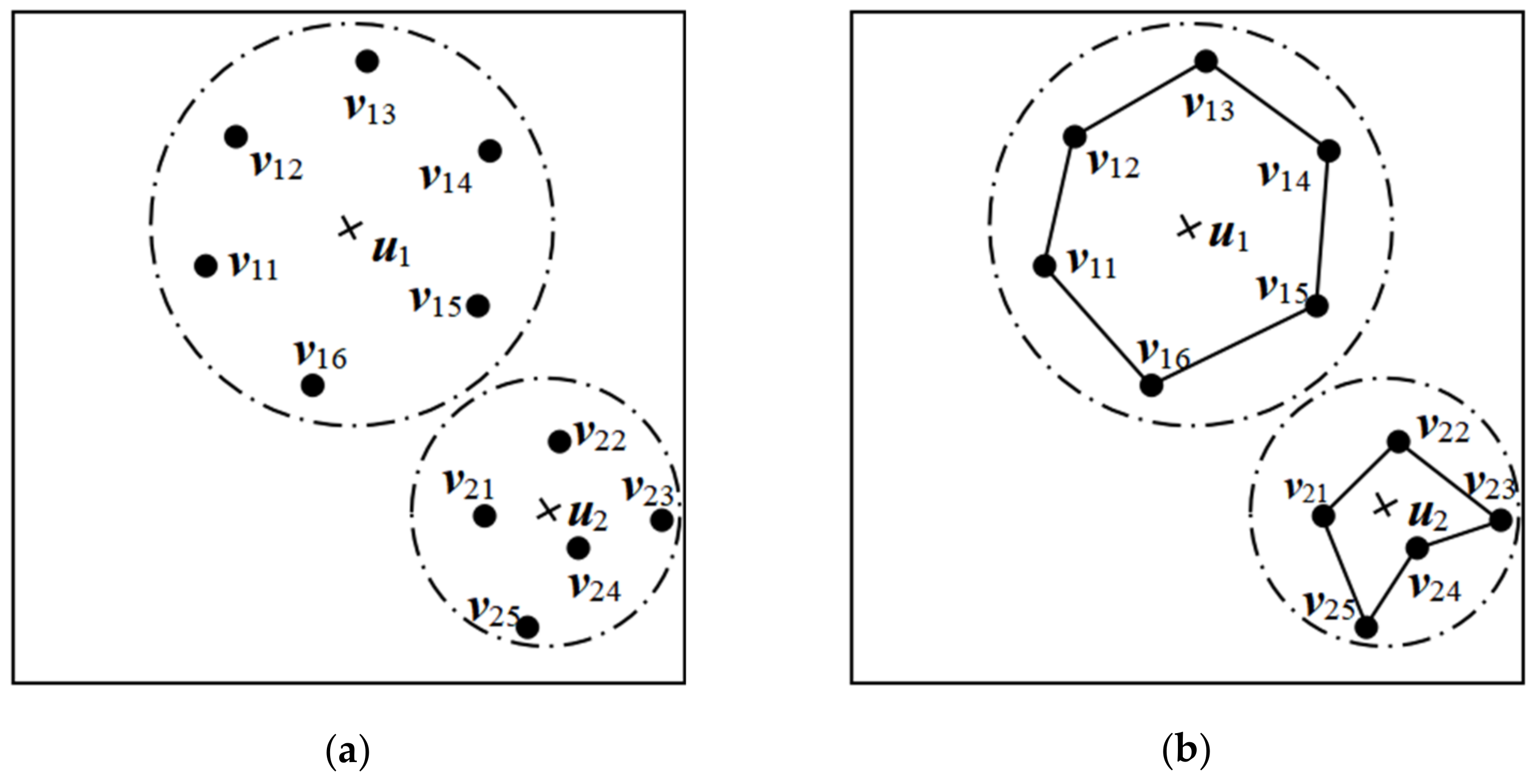
According to the mark clustering point process, the geometric model of the ground object in color remote sensing image is modeled. The mark clustering point process in data domain S is defined as W = (U, V), and its configuration is assumed to be w = (u, v). The configuration u = {u_j, j = 1, ..., m} of the parent process U defined on S is used to describe the location and spatial distribution of ground objects, where j is the index of ground objects, m is the number of objects, u_j = (u_1j, u_2j) ∈ S represents the position of the object j. The configuration of cluster sub-process V is defined as v = {v_j, j = 1, ..., m}, where v_j = {v_jg, g = 1, ..., k_j} is the cluster point set corresponding to random point u_j in the parent process, v_jg = (v_1jg, v_2jg) ∈ S is the coordinate of cluster point g corresponding to random point u_j, g is the cluster point index, and k_j is the number of cluster point corresponding to random point u_j. Each cluster point in the cluster point set v_j is connected in sequence to form the j-th polygon v_j, which is used to fit the geometry of the ground object, that is, the mark corresponding to the j-th ground object.

Figure 1 shows an example of modeling the geometry of a feature object using the mark clustering point process. Figure 1a shows the clustering point process. There are two parent processes u = {u₁, u₂}, represented by “+”. Taking the random point in the parent process (the “+” in the figure) as the center of the circle, two radii r₁ and r₂ are generated by Gaussian distribution. Generate the corresponding circular area (while generating the radius, ensure that the two circular areas do not intersect, to ensure that the two ground objects do not intersect in geographical location), to generate the sub-process. Each node in the sub-process is represented by “•”. As can be seen from the figure, v = {v₁, v₂}, v₁ = {v₁₁, v₁₂, v₁₃, v₁₄, v₁₅, v₁₆}, v₂ = {v₂₁, v₂₂, v₂₃, v₂₄, v₂₅}. Figure 1b shows the mark clustering point process based on Figure 1a. Taking the cluster points in each sub-process in Figure 1a as nodes and connecting them to form a simple polygon as the mark of the corresponding object. It can be seen that in this example, the sub-processes corresponding to the two-parent processes have six and five cluster points, respectively, to generate hexagon and pentagon.

2.2. Data Model of Image

The data domain S is divided into two categories, S = {S_o, S_b}, in which the object class is composed of m polygons, that is, S_o = {S_j, j = 1, …, m}, S_j is the area covered by the pixels contained in each polygon.

The pixel spectral measure value set in the region S_j is expressed as z_j= {z_i (x_i), x_i ∈ S_j}, and the pixel spectral measure value set in all object regions is expressed as z_o = {z_j , j = 1 ,..., m}. The set of pixel spectral measures in the background region is expressed as z_b = {z_i (x_i), x_i ∈ S_b}. Generally, assuming that the spectral measurement values of each pixel in the color remote sensing image obey the independent and same multivalued Gaussian distribution, the data model of color remote sensing image z under the condition of giving the mark clustering point process configuration w is,

$$\begin{array}{cc}p\left(\mathit{z}\left|\mathit{w},\theta \right.\right)\hfill & =\prod _{{\mathit{x}}_i\in {\mathit{S}}_b}p\left({\mathit{z}}_i\left|\mathit{w},\theta \right.\right)\times \prod _{j=1}^m\prod _{{\mathit{x}}_i\in {\mathit{S}}_j}p\left({\mathit{z}}_i\left|\mathit{w},\theta \right.\right)\hfill \\ & =\prod _{{\mathit{x}}_i\in {\mathit{S}}_b}\frac{1}{\sqrt{{\left(2\pi \right)}^3\left|{\mathit{\Sigma }}_b\right|}}\exp \left(-\frac{1}{2}{\left({\mathit{z}}_i-{\mathit{\mu }}_b\right)}^{\mathrm{T}}{\mathit{\Sigma }}_b^{-1}\left({\mathit{z}}_i-{\mathit{\mu }}_b\right)\right)\hfill \\ & \times \prod _{j=1}^m\prod _{{\mathit{x}}_i\in {\mathit{S}}_j}\frac{1}{\sqrt{{\left(2\pi \right)}^3\left|{\mathit{\Sigma }}_o\right|}}\exp \left(-\frac{1}{2}{\left({\mathit{z}}_i-{\mathit{\mu }}_o\right)}^{\mathrm{T}}{\mathit{\Sigma }}_o^{-1}\left({\mathit{z}}_i-{\mathit{\mu }}_o\right)\right)\hfill \end{array}$$

(1)

Among them, θ = (θ_b, θ_o) = (μ_b, Σ_b, μ_o, Σ_o) is the multivalued Gaussian distribution parameter, μ_b = (μ_bd, d = 1, ..., D)^T and Σ_b = [Σ_bdd’]_D×D is the mean vector and covariance matrix of multivalued Gaussian distribution obeyed by the pixel spectral measure in the background area, μ_o = (μ_od, d = 1, ..., D)^T and Σ_o = [Σ_odd’]_D×D is the mean vector and covariance matrix of multivalued Gaussian distribution obeyed by the pixel spectral measure of the object area.

Assuming that the components of θ are independent of each other, mean value μ_b and μ_o follow the multivalued Gaussian distribution with mean and covariance as (μ_μ, Σ_μ), covariance Σ_b and Σ_o follow the multivalued Gaussian distribution with mean and covariance as (μ_Σ, Σ_Σ). The prior probability of θ is,

$$\begin{array}{cc}\hfill & p\left(\mathit{\theta }\right)=p\left(\mathit{\mu }\right)p\left(\mathit{\Sigma }\right)=p\left({\mathit{\mu }}_b\right)p\left({\mathit{\mu }}_o\right)p\left({\mathit{\Sigma }}_b\right)p\left({\mathit{\Sigma }}_o\right)\hfill \\ \hfill & \times \frac{1}{\sqrt{{\left(2\pi \right)}^3\left|{\mathit{\Sigma }}_{\mu }\right|}}\exp \left(-\frac{1}{2}{\left({\mathit{\mu }}_b-{\mathit{\mu }}_{\mu }\right)}^{\mathrm{T}}{\mathit{\Sigma }}_{\mathit{\mu }}^{-1}\left({\mathit{\mu }}_b-{\mathit{\mu }}_{\mu }\right)\right)\times \frac{1}{\sqrt{{\left(2\pi \right)}^3\left|{\mathit{\Sigma }}_{\mu }\right|}}\exp \left(-\frac{1}{2}{\left({\mathit{\mu }}_o-{\mathit{\mu }}_{\mu }\right)}^{\mathrm{T}}{\mathit{\Sigma }}_{\mu }^{-1}\left({\mathit{\mu }}_o-{\mathit{\mu }}_{\mu }\right)\right)\hfill \\ \hfill & \times \frac{1}{\sqrt{{\left(2\pi \right)}^3\left|{\mathit{\Sigma }}_{\Sigma }\right|}}\exp \left(-\frac{1}{2}{\left({\mathit{\Sigma }}_b-{\mathit{\mu }}_{\Sigma }\right)}^{\mathrm{T}}{\mathit{\Sigma }}_{\Sigma }^{-1}\left({\mathit{\Sigma }}_b-{\mathit{\mu }}_{\Sigma }\right)\right)\times \frac{1}{\sqrt{{\left(2\pi \right)}^3\left|{\mathit{\Sigma }}_{\Sigma }\right|}}\exp \left(-\frac{1}{2}{\left({\mathit{\Sigma }}_o-{\mathit{\mu }}_{\Sigma }\right)}^{\mathrm{T}}{\mathit{\Sigma }}_{\Sigma }^{-1}\left({\mathit{\Sigma }}_o-{\mathit{\mu }}_{\Sigma }\right)\right)\hfill \end{array}$$

(2)

Among them, the distribution parameter μ_μ, Σ_μ, μ_Σ, and Σ_Σ can be specified according to the prior cognition of θ.

2.3. Ground Object Extraction Model

In this paper, the Bayesian theorem is used to model the ground object extraction model. Taking the image data model p(z | w, θ) as the probability model (likelihood function), combined with the prior probability p(θ) of distribution parameters and the prior model p(w) of the geometric configuration of the above-ground object.

The statistical laws of the location, distribution, and geometric shape of ground objects can be defined as the joint a priori probability distribution of the configuration (u, v, k, m) of the mark clustering point process by irregular graphics, that is, p(u, v, k, m), where k = {k_j, j = 1, ..., m}. Assuming that the prior probabilities describing the location and geometry of the ground object are independent of each other, p(u, v, k, m) can be written as,

$$p\left(\mathit{w}\right)=p\left(\mathit{u},\mathit{v},\mathit{k},m\right)\propto p\left(\mathit{u}|m\right)p\left(\mathit{v}|m,\mathit{k}\right)p\left(\mathit{k}|m\right)p\left(m\right)$$

(3)

Further assuming that each random point is independent of each other in the process of describing objects, and the geometric form of objects is also independent of each other, Equation (3) can be rewritten as,

$$\begin{array}{ll}p\left(\mathit{w}\right)& =p\left(\mathit{u},\mathit{v},k,m\right)\propto p\left(u|m\right)p\left(v|m,k\right)p\left(k|m\right)p\left(m\right)\\ & =p\left(m\right){\displaystyle \prod _{j=1}^{m}p\left(u_j\right)p\left(v_j\right)p\left(k_j\right)}\hfill \end{array}$$

(4)

This paper uses the cluster point process theory to model the location and geometric shape of ground objects. The clustering point process is a point process formed based on the Poisson point process. It is generally considered that its parent process is the Poisson process. Therefore, two conditions need to be met. One is that for the number of evenly distributed ground objects in the data domain S, it is generally considered that the variable appears randomly and independently at a fixed average rate, and it is considered to obey Poisson distribution. Then the probability distribution p(m) of the number of ground objects m can be expressed as,

$$p\left(m\right)=Poi\left(m;{\lambda }_m\right)=\frac{{\lambda }_m{}^m}{m!}\exp \left(-{\lambda }_m\right)$$

(5)

where Poi represents the Poisson distribution function and λ_m is the Poisson distribution parameter.

The other is that the location of ground objects in data domain S is generally considered to obey uniform distribution. That is, the probability distribution p(u_j) of the location of the j-th ground object follows the uniform distribution, which can be expressed as,

$$p\left(u_j\right)=Uni \left(\left|S\right|\right)={\left|S\right|}^{-1}$$

(6)

where, Uni represents uniform distribution and |S| represents the area of data domain S. At the same time, assuming that each object is independent of each other, the probability distribution p(u) of the location of all objects in the data domain S is expressed as,

$$p\left(u\right)={\displaystyle \prod _{j=1}^{m}p}\left(u_j\right)={\displaystyle \prod _{j=1}^{m}Uni\left(\left|S\right|\right)={\left|S\right|}^{-m}}$$

(7)

Since it is impossible for ground objects to overlap geographically, it is necessary to restrict the location and distribution of ground objects in the point process u to prevent different ground objects from occupying the same area. Therefore, the interaction probability function of the position of the ground object is defined as,

$$p\left(u,u\right)={\displaystyle \prod _{j=1}^{m-1}{\displaystyle \prod _{j\prime =j+1}^{m}p\left(u_j,u_{j\prime }\right)}}$$

(8)

where p(u_j, u_j’) is the probability distribution function of the interaction relationship between ground objects j and j’. In order to completely eliminate the overlap of ground objects j and j’, p(u_j, u_j’) can be defined as,

$$p\left(u_j,u_{j\prime }\right)=\left\{\begin{array}{l}0\hspace{1em}\hspace{1em}\left|S_j\cap S_{j\prime }\right|\ne \Phi \\ 1\hspace{1em}\hspace{1em} \mathrm{otherwise}\end{array}\right.$$

(9)

where S_j and S_j’ represent the area occupied by ground objects j and j’, and Φ represent an empty set.

After modeling the location and number of ground objects (parent process), we model the geometry of ground objects (sub-process). Then, assuming that the geometric configurations of objects are independent of each other, then,

$$p\left(v\right)={\displaystyle \prod _{j=1}^{m}p\left(v_j\right)}$$

(10)

For the cluster point set v_j = (v_jg, g = 1, ..., k_j) used to fit the geometric shape of the j-th ground object, assuming that the distribution of each cluster point is independent of each other, then,

$$p\left(v_j\right)={\displaystyle \prod _{g=1}^{k_j}p\left(v_{jg}\right)}$$

(11)

In order to express the clustering of each cluster point in the clustering sub-process to the position of each random point in the clustering parent process, it can be assumed that ||u_j-v_jg||₂ satisfies the Gaussian distribution,

$$p\left(v_{jg}\right)=G\left({‖u_j-v_{jg}‖}_2;{\mu }_v,{\sigma }_v\right)=\frac{1}{\sqrt{2\pi }{\sigma }_v}\exp \left(-\frac{{\left({‖u_j-v_{jg}‖}_2-{\mu }_v\right)}^2}{2{\sigma }_v^2}\right)$$

(12)

The number of cluster points k_j corresponding to the object j satisfies the Poisson distribution with parameter λ_k,

$$p\left(k_j\right)=Poi\left(k_j,{\lambda }_k\right)=\frac{{\lambda }_k^{k_j}}{k_j!}\exp \left(-{\lambda }_k\right)$$

(13)

Assuming that the geometric distribution of each object is independent of each other, the number of clustering sub-processes of each object is independent of each other. For the number of nodes on the whole remote sensing image k = {k_j, j = 1, ..., m}, the probability distribution function should be expressed as,

$$p\left(k\right)={\displaystyle \prod _{j=1}^{m}p\left(k_j\right)={\displaystyle \prod _{j=1}^{m}Poi\left(k_j,{\lambda }_k\right)={\displaystyle \prod _{j=1}^m\frac{{\lambda }_k^{k_j}}{k_j!}\exp \left(-{\lambda }_k\right)}}}$$

(14)

Then the final ground object extraction model (a posteriori probability model) p(w, θ | z) can be expressed as,

$$\begin{array}{ccc}p\left(\mathit{w},\theta |\mathit{z}\right)\hfill & \propto p\left(\mathit{z}|\mathit{w},\theta \right)p\left(\theta \right)p\left(\mathit{w}\right)\hfill & \\ & =\prod _{{\mathit{x}}_i\in \mathit{S}\setminus {\mathit{S}}_j}p\left({\mathit{z}}_i\left|\mathit{w},{\theta }_b\right.\right)\times \prod _{j=1}^m\prod _{{\mathit{x}}_i\in {\mathit{S}}_j}p\left({\mathit{z}}_i\left|\mathit{w},{\theta }_j\right.\right)\times p\left({\theta }_b\right)\times \prod _{j=1}^{m}p\left({\theta }_j\right)\hfill \\ & \times {\left|\mathit{S}\right|}^{-m}\times \prod _{j=1}^m\prod _{g=1}^{k_j}\left(\frac{1}{\sqrt{2\pi }{\sigma }_v}\exp \left(-\frac{{\left({∥{\mathit{u}}_j-{\mathit{v}}_{jg}∥}_2-{\mu }_v\right)}^2}{2{\sigma }_v^2}\right)\right)\hfill \\ & \times \prod _{j=1}^m\frac{{\lambda }_k^{k_j}}{k_j!}\exp \left(-{\lambda }_k\right)\times \frac{{{\lambda }_m}^m}{m!}\exp \left(-{\lambda }_m\right)\hfill \end{array}$$

(15)

2.4. Simulation and Optimization of Object Extraction Model

After the establishment of the object extraction model, the model needs to be simulated to obtain the optimal solution, to realize the object extraction based on remote sensing images. In this paper, the RJMCMC algorithm is used to simulate the ground object extraction (a posteriori probability) model, and the corresponding moving operation is designed to be combined with the MAP criterion to determine the location, quantity, and geometry of ground objects.

2.4.1. Simulation

Aiming at the ground object extraction (a posteriori probability) model based on the Bayesian theorem, the corresponding RJMCMC algorithm is designed. In addition to the parameters contained in the geometric configuration w of the ground object, the model should also include the distribution parameters θ of the distribution model obeyed by the remote sensing image observation data. Therefore, set all model parameters as Θ = (u, v, k, θ, m), and the posteriori probability model for extracting objects can be rewritten as,

$$\begin{array}{l}p\left(\Theta |z\right)\propto p\left(z|\Theta \right)p\left(\Theta \right)\\ p\left(u,v,k,\theta ,m|z\right)\propto p\left(z|u,v,k,\theta ,m\right)p\left(u|m\right)p\left(v|k,m\right)p\left(k|m\right)p\left(\theta |m\right)p\left(m\right)\end{array}$$

(16)

When the number of objects m and node-set k change, the dimension of model parameters Θ = (u, v, k, θ, m) will change. Therefore, the RJMCMC algorithm is used to simulate the object extraction model with variable dimensions. The basic idea is: to set the current sampling iteration indicator as t, and the corresponding model parameter set is Θ^(t). In the next iteration, the iteration indicator is t + 1, and the candidate parameters Θ^* are proposed according to the model parameters Θ^(t), that is, Θ^*=Θ^*(Θ^(t), ζ). The vector ζ is a continuous random vector defined to ensure the dimensional balance of Θ^* and Θ^(t), which meets the following requirements: |Θ^*| = |Θ^(t)| ± |ζ |, where | ⋅ | is the vector dimension. In order to completely fit the geometric shape of the ground object, the operation of changing the geometric shape of the ground object is designed. It mainly includes: updating distribution parameters θ, adding or deleting polygons, adding or deleting polygon nodes, and merging polygons.

Let the geometric configuration of the ground object under the current iteration number t state be w^(t) = {w_j^(t), j = 1, ..., m^(t)} = {u^(t), v^(t)} = {(u_j^(t), v_j^(t)), j = 1, ..., m^(t)}, where v_j^(t) = {v_jg, g = 1, ..., k_j^(t)}, k^(t) = {k_j^(t), j = 1, ..., m^(t)}. Accordingly, the distribution parameter is θ^(t) = {θ_b^(t), θ_j^(t), j = 1, ..., m^(t)}.

1.

Updating distribution parameters θ

The distribution parameters θ^(t) = (μ_b^(t), Σ_b^(t), μ_o^(t), Σ_o^(t)) are updated in sequence. Taking μ_b^(t) as an example, a new candidate parameter μ_b^* is proposed, and it is considered that it follows the Gaussian distribution with mean μ_b^(t) and variance ε_b, respectively. The acceptance rate of updating distribution parameter μ_b^(t) is defined as,

$$A({\theta }^{*},{\theta }^{{}^{\left(t\right)}})=\min \left\{1,\frac{p\left(z\left|{\theta }^{*},w^{\left(t\right)}\right.\right)p\left({\theta }^{*}\right)}{p\left(z\left|{\theta }^{\left(t\right)},w^{\left(t\right)}\right.\right)p\left({\theta }^{\left(t\right)}\right)}\right\}$$

(17)

We take the random number γ ~ Uni([0, 1]), if A(θ ^*, θ^(t)) ≥ γ, the operation of updating distribution parameters θ is accepted, θ^(t+1) = θ^*. Otherwise, the operation is rejected, θ^(t+1) = θ^(t).

2.

Add polygons

For add a polygon operation, let the geometric configuration of the ground object in the t-th iteration state be w^(t) = {w_j^(t), j = 1, ..., m^(t)} = {u^(t), v^(t)} = {(u_j^(t), v_j^(t)), j = 1, ..., m^(t)}. In the t+1-th iteration, add a polygon, the index of the newly added polygon is m^(t) + 1, and the configuration is $w_{m^{\left(t\right)}+1}^{*}=(u_{m^{\left(t\right)}+1}^{*},v_{m^{\left(t\right)}+1}^{*})$. Where, $u_{m^{\left(t\right)}+1}^{*}$~ Uni(S_b), $v_{m^{\left(t\right)}+1}^{*}=\{v_{m^{\left(t\right)}+1g}^{*},g=1,\dots ,k_{m^{\left(t\right)}+1}^{*}\}$,$v_{m^{\left(t\right)}+1g}^{*}~Uni(S_{m^{\left(t\right)}+1})$,$k_{m^{\left(t\right)}+1}^{*}~Poi\left({\lambda }_k\right)$. Then, satisfy: for arbitrary polygon v_j, j ∈ {1, ..., m^(t)}, $v_{m^{\left(t\right)}+1g}^{*}\cap v_j=\Phi$. After adding polygon operation, the candidate configuration of ground object geometry is $w^{*}=\{w^{\left(t\right)},w_{m^{\left(t\right)}+1}^{*}\}$. The distribution parameter corresponding to the newly added polygon is ${\theta }_{m^{\left(t\right)}+1}^{*}$, which is extracted from its predefined prior distribution. When a polygon is added, the distribution parameters θ^(t) of the ground object extraction model will not change, so its probability distribution will not change. However, the parameters (u^(t), v^(t), k^(t), m^(t)) in the geometric configuration w^(t) of the ground object will change with the increase in polygons, so the corresponding probability distribution will also change. At the same time, the remote sensing image data model p(z | θ^(t), w^(t)) will also change accordingly. Therefore, the acceptance rate of the operation of adding polygon is defined as,

$$\begin{array}{l}{A}_A\left(w^{*}\right)=\min \left\{1,R_{u^{+}}\right\}\\ R_{u^{+}}=\frac{p\left(z_{{}_{m^{(t)}+1}}^{*}\left|{\theta }_{m^{(t)}+1}^{(t)},w^{\left(t\right)}\right.\right)p\left(m^{\left(t\right)}+1\right)p\left(u^{*}|m^{\left(t\right)}+1\right)p\left(v^{*}|m^{\left(t\right)}+1,k^{*}\right)p\left(k^{*}|m^{\left(t\right)}+1\right)p_D}{p\left(z_{{}_{m^{(t)}+1}}^{*}\left|{\theta }_b^{(t)},w^{\left(t\right)}\right.\right)p\left(m^{\left(t\right)}\right)p\left(u^{\left(t\right)}|m^{\left(t\right)}\right)p\left(v^{\left(t\right)}|m^{\left(t\right)},k^{\left(t\right)}\right)p\left(k^{\left(t\right)}|m^{\left(t\right)}\right)p\left(\zeta \right)p_A}\end{array}$$

(18)

where, $\zeta =\left(w_{m^{\left(t\right)}+1}^{*},{\theta }_{m^{\left(t\right)}+1}^{*}\right)$ is the vector to keep the dimension balance, and p(ζ) is the probability function of the proposed vector. $z_{m^{\left(t\right)}+1}=\left\{z_i,x_i\in v_{m^{\left(t\right)}+1}^{*}\right\}$. p_D and p_A are the probability of selecting add or delete polygon operations, respectively. If one of these operations is not preferred in the design of the model simulation algorithm, we can assume p_D = p_A, that is, we can choose to add or delete polygons with equal probability.

We take the random number γ ~ Uni([0, 1]), if A_A(w^*) ≥ γ, the operation of add polygons is accepted, w^(t+1) = w^*. Otherwise, the operation is rejected, w^(t+1) = w^(t).

3.

Delete polygons

For delete a polygon operation, let the geometric configuration of the ground object in the t-th iteration state be w^(t) = {w_j^(t), j = 1, ..., m^(t)}. An arbitrary polygon v_j^(t) is randomly selected with equal probability 1/m^(t) from the current target geometric configuration w^(t). The geometric configuration of the selected polygon is w_j^(t) = (u_j^(t), v_j^(t)). We delete this polygon and reorder the remaining polygons. Then the geometric configuration of the object is w^* = {w_j^*, j = 1, ..., m^(t) − 1}. At the same time, the distribution parameters corresponding to this polygon are deleted θ_j^(t). When this operation is performed, the probability distribution of the distribution parameters θ^(t) remains unchanged. The parameters (u^(t), v^(t), k^(t), m^(t)) in the geometric configuration w^(t) of ground object and the remote sensing image data model p(z | θ^(t), w^(t)) will change. At the same time, this operation will also change the dimension of the parameter set. For simplicity, the optional vector to maintain dimensional balance is ζ = (w_j^(t), θ_j^(t)). Therefore, the acceptance rate of the operation of the deleting polygon is defined as,

$$\begin{array}{l}{A}_D\left(w^{*}\right)=\min \left\{1,R_{u^{-}}\right\}\\ R_{u^{-}}=\frac{p\left(z_j^{*}\left|{\theta }_b^{\left(t\right)},w^{\left(t\right)}\right.\right)p\left(m^{\left(t\right)}-1\right)p\left(u^{*}|m^{\left(t\right)}-1\right)p\left(v^{*}|m^{\left(t\right)}-1,k^{*}\right)p\left(k^{*}|m^{\left(t\right)}-1\right)p\left(\zeta \right)p_A}{p\left(z_j^{*}\left|{\theta }_j^{\left(t\right)},w^{\left(t\right)}\right.\right)p\left(m^{\left(t\right)}\right)p\left(u^{\left(t\right)}|m^{\left(t\right)}\right)p\left(v^{\left(t\right)}|m^{\left(t\right)},k^{\left(t\right)}\right)p\left(k^{\left(t\right)}|m^{\left(t\right)}\right)p_D}\end{array}$$

(19)

where, z_j= {z_i, x_i∈ v_j}.

We take the random number γ ~ Uni([0, 1]), if A_D(w^*) ≥ γ, the operation of delete polygons is accepted, w^(t+1) = w^*. Otherwise, the operation is rejected, w^(t+1) = w^(t).

Figure 2 is the examples of adding and deleting polygons, where the Figure 2a shows the geometric configuration w^(t) of the ground object at time t. Furthermore, Figure 2b,c show examples of adding or deleting a polygon at time t + 1, respectively.

4.

Add polygon nodes

For any given polygon, the neighborhood node of any node is the node directly connected with the node, and the two directly connected nodes form a neighborhood node pair. Let the geometric configuration of the ground object in the t-th iteration state be w^(t) = {w_j^(t), j = 1, ..., m^(t)}. An arbitrary polygon v_j^(t) is randomly selected with equal probability 1/m^(t) from the current target geometric configuration w^(t). Select a neighborhood node pair (v_jg^(t), v_jg+1^(t)) with equal probability 1/k_j^(t) from the node set v_j^(t) of the selected polygon. A point is randomly selected as an additional candidate node in the intersection area between the circle with (v_jg^(t) + v_jg+1^(t))/2 as the center |v_jg^(t) + v_jg+1^(t)|/2 as the radius and the visible area of edge v_jg^(t)v_jg+1^(t). Then, the candidate node is inserted between the node pairs (v_jg^(t), v_jg+1^(t)) to construct the candidate polygon v_j^*. Finally, the nodes of the candidate polygon v_j^* are reordered as v_j^* = {v_jg^*, g = 1, ..., k_j^(t) + 1}. Without losing generality, record the new node as v_jg^*. When this operation is performed, the probability distributions of the distribution parameters θ^(t) and the parameters (u^(t), m^(t)) in the geometric configuration w^(t) of the ground object remain unchanged. The probability distribution of (v^(t), k^(t)) parameters and remote sensing image data model p(z| θ^(t), w^(t)) will change. At the same time, this operation will also change the dimension of the parameter set. For simplicity, the optional vector to keep the dimension balance is ζ = {v_jg^*}. The acceptance rate of the operation of adding polygon node is defined as,

$$A_{AV}\left(v^{*},v^{\left(t\right)}\right)=\min \left\{1,\frac{p\left(z_j^{*}|{\theta }_j^{\left(t\right)}\right)p\left(z_{bj}^{*}|{\theta }_b^{\left(t\right)}\right)p\left(k_j^{\left(t\right)}+1\right)p\left(v^{*}\right)p_{DV}}{p\left(z_j^{*}|{\theta }_b^{\left(t\right)}\right)p\left(z_{bj}^{*}|{\theta }_j^{\left(t\right)}\right)p\left(k_j^{\left(t\right)}\right)p\left(v^{\left(t\right)}\right)p\left(\zeta \right)p_{AV}}\right\}$$

(20)

where z_j^* = S_j^* \ S_j^(t), z_bj^* = S_j^(t) \ S_j^*, S_j^* and S_j^(t) represent the areas occupied by the candidate polygon v_j^*and the current polygon v_j^(t), respectively. If z_j^* or z_bj^* is an empty set, we set its corresponding conditional probability density function to 1. p_DV and p_AV are the probability of selecting add or delete polygon node operations, respectively.

We take the random number γ ~ Uni([0, 1]), if A_AV(v_j^*, v_j^(t)) ≥ γ, the operation of add a polygon node is accepted, w^(t+1) = w^*. Otherwise, the operation is rejected, w^(t+1) = w^(t).

5.

Delete polygon nodes

Let the geometric configuration of the ground object in the t-th iteration state be w^(t) = {w_j^(t), j = 1, ..., m^(t)}. An arbitrary polygon v_j^(t) is randomly selected with equal probability 1 / m^(t) from the current target geometric configuration w^(t). Then, a node is randomly selected from the polygon node set v_j^(t) with equal probability 1 / k_j^(t) and recorded as v_jg^(t). If the two neighborhood nodes of the node v_jg^(t) are visible to each other, delete the node and reorder the remaining nodes v_j^* = {v_jg^*, g = 1, ..., k_j^(t) − 1} to build the candidate polygon v_j^*.

When this operation is performed, the probability distributions of the distribution parameters θ^(t) and the parameters (u^(t), m^(t)) in the geometric configuration w^(t) of the ground object remain unchanged. The probability distribution of (v^(t), k^(t)) parameters and remote sensing image data model p(z| θ^(t), w^(t)) will change. At the same time, this operation will also change the dimension of the parameter set. For simplicity, the optional vector to keep the dimension balance is ζ = {v_jg^*}. The acceptance rate of the operation of deleting polygon node is defined as,

$$A_{DV}\left(v^{*},v^{\left(t\right)}\right)=\min \left\{1,\frac{p\left(z_j^{*}|{\theta }_j^{\left(t\right)}\right)p\left(z_{bj}^{*}|{\theta }_b^{\left(t\right)}\right)p\left(k_j^{\left(t\right)}-1\right)p\left(v^{*}\right)p\left(\zeta \right)p_{AV}}{p\left(z_j^{*}|{\theta }_b^{\left(t\right)}\right)p\left(z_{bj}^{*}|{\theta }_j^{\left(t\right)}\right)p\left(k_j^{\left(t\right)}\right)p\left(v^{\left(t\right)}\right)p_{DV}}\right\}$$

(21)

We take the random number γ ~ Uni([0, 1]), if A_DV(v_j^*, v_j^(t)) ≥ γ, the operation of delete a polygon node is accepted, w^(t+1) = w^*. Otherwise, the operation is rejected, w^(t+1) = w^(t).

Figure 3 is the example of adding and deleting a polygon node, where Figure 3a shows the geometric configuration w^(t) of the ground object at time t. Furthermore, Figure 3b,c show examples of adding or deleting a polygon node at time t + 1, respectively.

6.

Merging polygons

Let the geometric configuration of the ground object in the t-th iteration state be w^(t) = {w_j^(t), j = 1, ..., m^(t)}. Select two polygons v_j^(t) and v_j’^(t) randomly from the current object geometric configuration w^(t), and then calculate their node pair spacing, respectively. If the distance between the shortest and sub-shortest node pairs is less than a given threshold, we merge the two polygons. The merging polygon operation is realized by merging the node pairs. Take the middle point of the shortest node pair and the sub-shortest node pair as the newly added nodes and combine them with other nodes to construct the candidate polygon v_j^*. When this operation is performed, the distribution parameters θ^(t) remain unchanged, and its probability distribution remains unchanged. The parameters (u^(t), v^(t), k^(t), m^(t)) in the geometric configuration w^(t) of the ground object will change with the merging of polygons and their corresponding probability distribution will also change. At the same time, the remote sensing image data model p(z | θ^(t), w^(t)) will also change, so the acceptance rate of merging polygons operation is,

$$\begin{array}{l}{A}_M\left(w^{*}\right)=\min \left\{1,R_M\right\}\\ R_M=\frac{p\left(z_j^{*}|{\theta }_j^{\left(t\right)}\right)p\left(z_{bj}^{*}|{\theta }_b^{\left(t\right)}\right)p\left(m^{\left(t\right)}-1\right)p\left(u^{*}|m^{\left(t\right)}-1\right)p\left(v^{*}|m^{\left(t\right)}-1,k^{*}\right)p\left(k^{*}|m^{\left(t\right)}-1\right)}{p\left(z_j^{*}|{\theta }_b^{\left(t\right)}\right)p\left(z_{bj}^{*}|{\theta }_j^{\left(t\right)}\right)p\left(m^{\left(t\right)}\right)p\left(u^{\left(t\right)}|m^{\left(t\right)}\right)p\left(v^{\left(t\right)}|m^{\left(t\right)},k^{\left(t\right)}\right)p\left(k^{\left(t\right)}|m^{\left(t\right)}\right)}\end{array}$$

(22)

where, z_j^* = S_j^*\(S_j^(t)∪S_j’^(t)),z_bj^* = (S_j^(t)∪S_j’^(t))\S_j^*.

We take the random number γ ~ Uni([0, 1]), if A_M(w^*) ≥ γ, the operation of merge polygons is accepted, w^(t+1) = w^*. Otherwise, the operation is rejected, w^(t+1) = w^(t).

Figure 4 is an example of merge polygons, whereas Figure 4a shows the geometric configuration w^(t) of the ground object at time t. Furthermore, Figure 4b shows the example of merging polygons at time t + 1.

2.4.2. Optimization

MAP criterion is the simplest optimization scheme. When the posterior probability in the Bayesian extraction model is the largest, the corresponding solution is the optimal object extraction result. The optimal parameter estimation solution under MAP condition is,

$$\left(\widehat{w},\widehat{\theta }\right)=\arg \underset{\left(w,\theta \right)}{\max } p\left(w,\theta |z\right)$$

(23)

where $\widehat{\Theta }=\left(\widehat{w},\widehat{\theta }\right)=\left(\widehat{u},\widehat{v},\widehat{k},\widehat{m},\widehat{\theta }\right)$ is the maximum a posteriori probability estimate of the parameter set (w, θ) = (u, v, k, m, θ).

Among the above parameters, u = {u_j= (u_1j, u_2j) ∈ S, j = 1, ..., m}, where u_j = (u_1j, u_2j) represents the position of object j, and m represents the number of objects. v = {v_j, j = 1, ..., m}, where v_j = {v_jg, g = 1, ..., k_j} is the node coordinate set corresponding to the object j. Therefore, the configuration w = (u, v) of the mark clustering point process can completely describe the extracted ground object.

3. Experiment Results

In order to verify the accuracy of the proposed algorithm quantitatively and qualitatively, synthetic and real color remote sensing images are used for experiments.

3.1. Synthetic Image Experiment

According to the given template image (as shown in Figure 5a), two ground object types of forest land and bare land are spliced to generate a 256 × 256 pixels image (as shown in Figure 5b). The blue line in Figure 5c is the outline of the object.

The proposed algorithm is used to extract ground objects from the synthetic image in Figure 5b. During the experiment, if the number of iterations is set too much, it will cause time redundancy. If the number of iterations is small, the algorithm will not converge, and the fitting of the geometric features of the object will not be completed. After many experiments, the number of iterations in this paper is set to 4000. We conducted experiments on the Intel (R) Core (TM) i7-10510u CPU @ 1.80GHz 2.30 GHz device, and the running time was about 303.403035 s.

During the experiment, each iteration performs six designed operations, of which the last five operations will affect the geometry of the polygon used to fit the objects.

Table 1. Number of times the move operation was accepted.

Move Operation	Number of Times the Move Operation Was Accepted
Add polygons	4
Delete polygons	3
Add polygon nodes	683
Delete polygon nodes	616
Merging polygons.	1

lists the number of times each move operation is accepted. Among them, the operations of adding polygons, deleting polygons, and merging polygons are used to determine the number of objects and are accepted fewer times. The operations of adding polygon nodes and deleting polygon nodes are used to adjust the shape of polygons and are accepted more times.

Figure 6 shows the acceptance rate of the last five operations. Among them, the polygon addition operation was accepted four times, which occurred in iterations 26, 49, 62, and 78, respectively, as shown in Figure 6a. The polygon deletion operation was accepted three times, which occurred in iterations 2, 4, and 185, respectively, as shown in Figure 6b. The merge polygon operation is accepted once, which occurs in the 581st iteration, as shown in Figure 6e. These three operations are used to determine the number of objects. Adding and deleting polygon nodes are accepted more times, 683 times and 616 times, respectively, as shown in Figure 6c,d to adjust the geometry of the polygon.

The total number of iterations of the experiment is 4000, and the object extraction results are displayed every 20 times, as shown in Figure 7. Among them, Figure 7a shows the initialization result. During the initialization process, the number of given parent processes is 4, which is represented by the green cross wire in the figure, and the given clustering range is represented by the blue circle in the figure. The sub-processes corresponding to the parent process are generated within the blue circle. The number of sub-processes is set to 4, which is represented by solid red dots in the figure. Connect the sub-processes corresponding to each parent process in sequence to form an initial polygon, as shown by the red line, to form an initialization result. Figure 7b shows the results of the 20th iteration. Compared with the initialization results (Figure 7a), it is found that in the first 20 iterations, the add polygon operation is not accepted, and the delete polygon operation is accepted twice, which occurs in the second and fourth iterations, respectively. Figure 7c shows the results of the 40th iteration. Compared with Figure 7b, it is found that in the 20 iterations, a polygon is added, which occurs in the 26th iteration, and the polygon deletion operation is not received. Figure 7d shows the results of the 60th iteration. Compared with Figure 7c, it is found that in the 20 iterations, a polygon is added, which occurs in the 49th iteration, and the polygon deletion operation is not received. Figure 7e shows the results of the 80th iteration. Compared with Figure 7d, it is found that in the 20 iterations, the polygon addition operation is accepted twice, which occurs in the 62nd and 78th iterations, respectively, and the polygon deletion operation is not accepted. Figure 7f shows the results of the 200th iteration. Compared with Figure 7e, it is found that one polygon deletion operation is accepted, which occurs in the 185th iteration. Figure 7g shows the result of the 580th iteration. Compared with Figure 7f, the operations of adding and deleting polygons are not accepted, but the geometry of polygons is adjusted by adding and deleting polygon nodes. Figure 7h shows the results of the 600th iteration. Compared with Figure 7g, it is found that a polygon merging operation is accepted, which occurs in the 581st iteration. The polygon geometry is adjusted by continuously adding and deleting nodes to form the final object extraction result, as shown in Figure 7i. It can be seen that after adding, deleting, and merging polygons, the final number of polygons is consistent with the object number of figures.

The final experimental results are shown in Figure 8, in which Figure 8a is to convert the object extraction results into segmentation results in order to quantitatively evaluate the experimental results by using the confusion matrix method. Figure 8b shows the superposition results of the extracted ground object contour and the experimental image to qualitatively evaluate the experimental results. Figure 8c shows the extracted contour line of the ground object. The solid green dots in the figure represent each node, and the solid red lines are used to connect each node in order to form a polygon. According to the final experimental results, the central, quadrilateral, pentagonal, and elliptical objects are connected by 23, 13, 23, and 21 nodes, respectively.

The proposed method belongs to the statistical method of traditional methods. Statistical methods are usually divided into pixel processing units and object-oriented processing units. Therefore, in order to verify the effectiveness of the experiment, the paper first uses the statistical method in which the pixel is the processing unit for comparison [18]. Secondly, the comparison is made by using the mark point process method, which takes the object as the processing unit but only uses the regular rectangle as the mark [19]. At last, the method based on the active–active contour model, which is commonly used in traditional methods, is used for comparison [20]. The experimental results of the three comparison algorithms are shown in Figure 9. In order to quantitatively evaluate the experimental results by using the confusion matrix, the segmentation results of the three algorithms are obtained, as shown in Figure 9a1–c1. In order to qualitatively evaluate the experimental results visually, the object extraction results of the three algorithms are superimposed with the experimental images, as shown in Figure 9a2–c2. The experimental results show that the algorithms based on pixel and active contour model have a good segmentation effect on bare land with uniform spectral measurement, but for forest areas with uneven spectral measurement, a lot of noise will be generated in the experimental results. The method based on the rule mark point process has a good positioning effect on bare ground objects but a poor geometric fitting effect.

Take the template image (Figure 5a) as the standard image, and take the segmentation results of the proposed algorithm and three comparison algorithms (Figure 8a and Figure 9a1–c1) as the experimental image to establish the confusion matrix. Then calculate the accuracy index according to the confusion matrix, and the results are shown in

Table 2. Synthetic image quantitative evaluation.

	Proposed Algorithm/Pixel-Based Algorithm/Rule Mark Point Process/Active Contour Model
	C1	C2
User accuracy (%)	99.91/52.68/90.61/98.23	98.25/99.91/98.14/99.64
Product ccuracy (%)	89.13/99.54/88.58/98.23	99.99/85.38/98.50/79.09
Total accuracy (%)	98.46/87.37/97.10/81.78
Kappa coefficient	0.933/0.619/0.879/0.506
F1 measurement (%)	94.22/68.90/89.58/60.25

. It can be seen from the table that the user accuracy of the background area and the product accuracy of the object area that are based on the pixel algorithm and the active contour model algorithm are higher than the proposed algorithm. This is because the spectral measure distribution of the object area is relatively uniform, so the two algorithms have better segmentation results for the object area. However, for the background region with complex spectral measure distribution, the two algorithms will produce a lot of noise, which reduces the overall accuracy of the experimental results. Although the rule mark point process algorithm will not produce a lot of noise, its overall accuracy is also affected because of its poor-fitting effect on the boundary of ground objects. In general, the proposed algorithm is superior to the other three comparison algorithms in terms of total accuracy, kappa coefficient, and F1 measurement.

3.2. Real Image Experiment

In order to avoid the over-idealization of quantitative analysis of experimental results using only synthetic images, two real remote sensing images [21] with islands and lakes as objects are selected for the ground object extraction experiment. The boundary line is determined by visual analysis through human observation. Because there will be some errors in the object boundary line determined by human vision, only the remote sensing image with one object is selected in the experiment. As shown in Figure 10, Figure 10b1,b2 are remote sensing images of islands and lakes, respectively. Figure 10c1,c2 are the manually determined object boundaries (solid blue line in the figure). Figure 10a1,a2 are standard image templates for artificially determined object boundaries to quantitatively evaluate the experimental results.

The proposed algorithm is used to experiment in Figure 10b1,b2, and the experimental results are shown in Figure 11. Among them, Figure 10c1,c2 are the object extraction results. The solid green dots in the figure represent the nodes used to form the polygon, and the number of nodes is 35 and 44, respectively. Each group of nodes is sequentially connected with solid red lines to form polygons, which are used to fit island and lake objects, respectively. The formed polygon is superimposed with the experimental image (Figure 10b1,b2) for visual evaluation. The superposition results are shown in Figure 11b1,b2. It can be seen from the figure that the polygon formed by the experimental results can not only locate the island and lake but also accurately fit their geometry. In order to quantitatively evaluate the experimental results, the extracted object results are converted into segmentation results, as shown in Figure 11a1,a2.

We also use three comparison algorithms to experiment with Figure 10b1,b2, and the experimental results are shown in Figure 12. Figure 12a1–c1 shows the segmentation results of the three comparison algorithms on the island image and Figure 12a2–c2 shows the object extraction results of the three comparison algorithms on the island image. In the island image, comparing the island object with the background, it can be seen that the spectral measure distribution in the background area is more uniform than that in the target area. Therefore, in the experimental results based on pixel and active contour algorithm, the object area produces more noise, while in the background area, there is noise only in some areas with uneven spectral measure distribution. Figure 12a3–c3 shows the segmentation results of the three comparison algorithms on the lake image and Figure 12a4–c4 shows the object extraction results of the three comparison algorithms on the lake image. In the lake image, the distribution of pixel spectral measures in the lake area is more uniform than that in the background area. Therefore, in the experimental results based on pixel and active contour algorithm, more noise is generated in the background area. The rule mark point process algorithm will not produce noise, but the fitting effect of the boundary of the object area is not ideal, whether for the island image with complex object distribution or the lake image with complex background distribution.

We compare the standard images of the island image and lake image (as shown in Figure 10a1,a2) and the segmentation results of the four methods (as shown in Figure 11a1,a2 and Figure 12a1–c1,a3–c3) to establish the confusion matrix. Each accuracy index is calculated according to the confusion matrix, and the calculation results are shown in

Table 3. Quantitative evaluation of island and lake images.

Precision Index	Image	Proposed Algorithm/Pixel-Based Algorithm/Rule Mark Point Process/Active Contour Model
		C1	C2
User accuracy (%)	Island image	97.87/10.53/69.69/36.13	99.61/89.53/99.73/93.76
	Lake Image	99.82/25.00/67.52/25.66	99.33/99.99/99.93/99.99
Product ccuracy (%)	Island image	96.67/45.06/97.81/49.01	99.75/55.09/95.01/89.84
	Lake Image	94.52/99.96/99.49/99.94	99.98/62.81/94.06/64.08
Total accuracy (%)	Island image	99.43/54.04/95.30/85.55
	Lake Image	99.38/66.91/94.66/68.04
Kappa coefficient	Island image	0.969/0.001/0.788/0.336
	Lake Image	0.968/0.271/0.775/0.282
F1 measure	Island image	97.27/17.07/81.39/41.59
	Lake Image	97.10/40.00/80.44/40.83

. In the results of the pixel algorithm and active contour algorithm, only the user accuracy of the background area and the product accuracy of the object area in the lake image are high. This is because the pixel spectral measure distribution in the object area of the lake image is relatively uniform. Compared with the object area of the lake image, the distribution of spectral measures is more complex, which leads to low result accuracy and reduces the overall accuracy of the two algorithms. The accuracy of the rule mark point process algorithm is mostly better than these two algorithms, so the total accuracy is also better than these two algorithms. For the proposed algorithm, although the user accuracy of the background area and the product accuracy of the object area in the lake image may be lower than the three comparison algorithms, the other accuracy is higher, which improves the overall accuracy of the algorithm. It can also be seen from the total accuracy, kappa coefficient, and F1 measure that the proposed algorithm is significantly better than the three comparison algorithms.

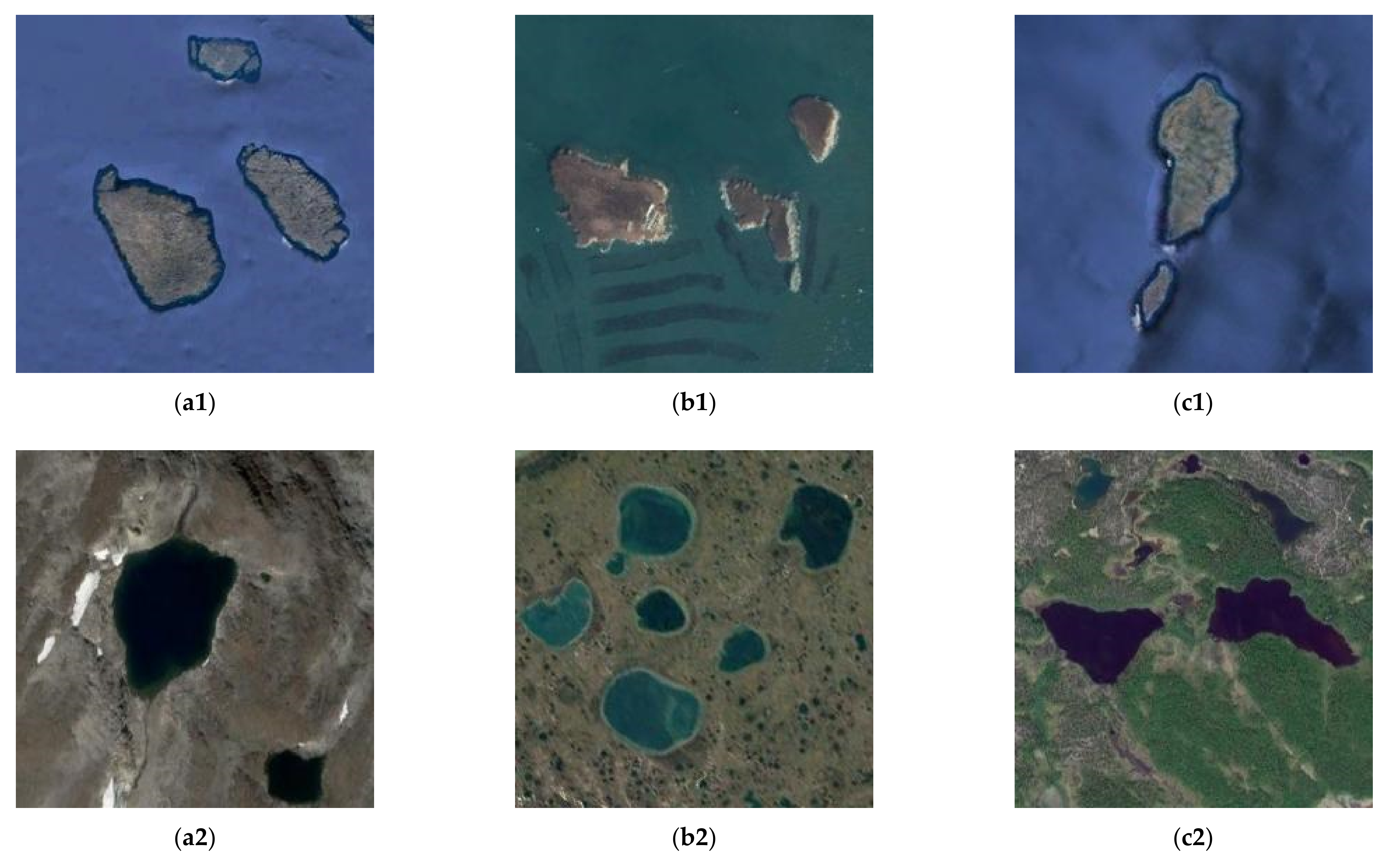
Figure 13 shows six images selected from the aerospace remote sensing object detection data set [21] marked by Northwest University of technology, all of which are 256 × 256 pixels. Figure 13a1–c1 shows three island images, and Figure 13a2–c2 shows three lake images. It can be seen from the image that the spectral measures of the pixels in the background area of the three island images are evenly distributed, and the spectral measures of the object pixels are quite different. The spectral measure distribution of the pixels in the background area of the three lake images is more complex, while the spectral measure distribution of the object pixels is more uniform. The geometric shapes of the objects in these six images show irregular characteristics.

The proposed algorithm is used to experiment with the remote sensing image in Figure 13. The experimental results are shown in Figure 14. In the figure, the solid green dots represent the nodes constituting the ground object geometry, and the solid red lines represent the extracted object geometry. Among them, Figure 14a1–c1 shows the results of extracting island objects, and the number of extracted objects is four, three, and two, respectively, which is the same as the visual interpretation results in the experimental image. Figure 14a2–c2 shows the extracted lake results, and the number of extracted objects is two, six, and four, respectively. The extraction results of the first two images are consistent with the visual interpretation results, while the number of surface objects visually interpreted in Figure 14c2 should be 3. In the experimental results, two polygons are used to fit a lake object.

The object extraction results are superimposed with the experimental images for qualitative evaluation, as shown in Figure 15. The proposed algorithm can not only accurately locate the object but also accurately fit its geometry for both island images and lake images. When a polygon cannot be used to fit an object, the algorithm will automatically detect multiple polygons to fit a ground object.

In this paper, the pixel-based image processing method is used to experiment with the six remote sensing images in Figure 13. The experimental results are shown in Figure 16. Among them, Figure 16a1–c1 show the experimental results of three island images. The pixel spectral measurement values in the object area are greatly different, while the pixel spectral measurement values in the background area are relatively small compared with the object area, which makes more noise in the object area and less noise in the back area, especially in Figure 16c1. Figure 16a2–c2 shows the experimental results of three lake images. The pixel spectral measurement values in the background area have a large difference, while the pixel spectral measurement values in the target area have a small difference relative to the background area. Therefore, in the experimental results, the noise in the object area is relatively less, and the noise in the background area is relatively more.

In this paper, the mark point process algorithm with a rectangle as a mark is used to experiment on six images. The experimental results are shown in Figure 17. Figure 17a1–c1 shows the experimental results of three island images, and the number of extracted ground objects are three, four, and two, respectively. Figure 17a2–c2 shows the experimental results of three lake images, and the number of ground objects extracted are two, six, and three, respectively. The geometric shape of the object extracted by this algorithm is rectangular because the pre-defined mark of this algorithm is rectangular. A rectangle is difficult to fit the ground object with irregular geometric characteristics, which reduces the overall accuracy of the experimental results.

In this paper, the algorithm based on the active contour model is used to experiment on six images. The experimental results are shown in Figure 18. It can be seen from the experimental results that there will be more noise in the experimental results of the algorithm for island images with large differences in pixel spectral measurements in the object area and lake images with large differences in pixel spectral measurements in the background area. Although there is less noise than in the pixel-based algorithm, the positions of the noisy images are basically the same. Therefore, it can be seen that whether the algorithm is based on a pixel or active contour model, it is difficult to achieve a more accurate object extraction effect for the regions with large differences in pixel spectral measures.

4. Conclusions

In view of the irregularity of the geometric shape of the ground object in remote sensing image, based on the theory of random geometric point process, this paper proposes a new ground object extraction method based on the mark clustering point process and expresses the position, distribution, and geometric shape of the ground object. In this paper, the traditional statistical method is used for detection, which requires a lot of sampling work, so the experimental speed is slow. Therefore, in the experiment, only small image objects with obvious irregular geometry are fitted with geometric features. In future work, we can consider how to quickly realize the object detection of large images or images with more complex scenes.

References

- Foschini, G.J.; Gans, M.J. On limits of wireless communications in a fading environment when using multiple antennas. Wirel. Pers. Commun. 1998, 6, 311–335. [Google Scholar] [CrossRef]
- Masuda, R.; Inoue, R. Point event cluster detection via the Bayesian generalized fused lasso. ISPRS Int. J. Geo-Inf. 2022, 11, 187. [Google Scholar] [CrossRef]
- Haroon, M.; Shahzad, M.; Fraz, M.M. Multisized object detection using spaceborne optical imagery. IEEE J. Sel. Top. Appl. Earth Obs. Remote Sens. 2020, 13, 3032–3046. [Google Scholar] [CrossRef]
- Erus, G.; Loménie, N. How to involve structural modeling for cartographic object recognition tasks in high-resolution satellite images. Pattern Recognit. Lett. 2010, 31, 1109–1119. [Google Scholar] [CrossRef] [Green Version]
- Xu, Y.; Xiong, W.; Liu, J. A new ship target detection algorithm based on SVM in high resolution SAR images. In Proceedings of the International Conference on Advances in Image Processing, Bangkok, Thailand, 25–27 August 2017. [Google Scholar]
- Yokoya, N.; Iwasaki, A. Object detection based on sparse representation and Hough voting for optical remote sensing imagery. IEEE J. Sel. Top. Appl. Earth Obs. Remote Sens. 2015, 8, 2053–2062. [Google Scholar] [CrossRef]
- Chen, H.; Gao, T.; Qian, G.; Chen, W.; Zhang, Y. Tensored generalized hough transform for object detection in remote sensing images. IEEE J. Sel. Top. Appl. Earth Obs. Remote Sens. 2020, 13, 3503–3520. [Google Scholar] [CrossRef]
- Sun, H.; Sun, X.; Wang, H.; Li, Y.; Li, X. Automatic target detection in high-resolution remote sensing images using spatial sparse coding bag-of-words model. IEEE Geosci. Remote Sens. Lett. 2011, 9, 109–113. [Google Scholar] [CrossRef]
- Baddeley, A.J.; Lieshout, M.N.M.V. Stochastic geometry models in high-level vision. J. Appl. Stat. 1993, 20, 231–256. [Google Scholar] [CrossRef]
- Pievatolo, A.; Green, P.J. Boundary detection through dynamic polygons. J. R. Stat. Soc.: Ser. B (Stat. Methodol.) 1998, 60, 609–626. [Google Scholar] [CrossRef]
- Zhao, Q.; Zhang, H.; Li, Y. Detecting dark spots from SAR intensity images by a point process with irregular geometry marks. Int. J. Remote Sens. 2019, 40, 774–793. [Google Scholar] [CrossRef]
- Descombes, X.; Zerubia, J. Marked point process in image analysis. IEEE Signal Process. Mag. 2002, 19, 77–84. [Google Scholar] [CrossRef] [Green Version]
- Ortner, M.; Descombes, X.; Zerubia, J. Building outline extraction from digital elevation models using marked point processes. Int. J. Comput. Vis. 2007, 72, 107–132. [Google Scholar] [CrossRef]
- Perrin, G.; Descombes, X.; Zerubia, J. A marked point process model for tree crown extraction in plantations. In Proceedings of the IEEE International Conference on Image Processing, Genova, Italy, 14 September 2005. [Google Scholar]
- Lacoste, C.; Descombes, X.; Zerubia, J. Point processes for unsupervised line network extraction in remote sensing. IEEE Trans. Pattern Anal. Mach. Intell. 2005, 27, 1568–1579. [Google Scholar] [CrossRef] [PubMed]
- Ortner, M.; Descombes, X.; Zerubia, J. A marked point process of rectangles and segments for automatic analysis of digital elevation models. IEEE Trans. Pattern Anal. Mach. Intell. 2007, 30, 105–119. [Google Scholar] [CrossRef] [PubMed] [Green Version]
- Lafarge, F.; Gimel’Farb, G.; Descombes, X. Geometric feature extraction by a multimarked point process. IEEE Trans. Pattern Anal. Mach. Intell. 2009, 32, 1597–1609. [Google Scholar] [CrossRef] [PubMed] [Green Version]
- Scherrer, B.; Dojat, M.; Forbes, F.; Garbay, C. Agentification of Markov model-based segmentation: Application to magnetic resonance brain scans. Artif. Intell. Med. 2009, 46, 81–95. [Google Scholar] [CrossRef] [PubMed] [Green Version]
- Li, Y.; Li, J. Oil spill detection from SAR intensity imagery using a marked point process. Remote Sens. Environ. 2010, 114, 1590–1601. [Google Scholar] [CrossRef]
- Ding, K.; Xiao, L.; Weng, G. Active contours driven by local pre-fitting energy for fast image segmentation. Pattern Recognit. Lett. 2018, 104, 29–36. [Google Scholar] [CrossRef]
- Cheng, G.; Han, J.; Lu, X. Remote sensing image scene classification: Benchmark and state of the art. Proc. IEEE 2017, 105, 1865–1883. [Google Scholar] [CrossRef] [Green Version]
Figure 1.
Mark clustering point process to model ground object geometry: (a) The clustering point process; (b) The mark clustering point process.
Figure 2.
The examples of adding and deleting a polygon: (a) Configuration w(t) of object; (b) Add a polygon; (c) Delete a polygon.
Figure 3.
The examples of adding and deleting a polygon node: (a) Configuration w(t) of object; (b) Add a polygon node; (c) Delete a polygon node.
Figure 4.
The example of merge polygons: (a) Configuration w(t) of object; (b) Merge polygons.
Figure 5.
Synthetic images: (a) Template image; (b) Synthetic image; (c) Standard contour.
Figure 6.
Acceptance rates of different operations during iteration: (a) The acceptance rate of add polygons; (b) The acceptance rate of delete polygons; (c) The acceptance rate of add polygon nodes; (d) The acceptance rate of delete polygon nodes; (e) The acceptance rate of merging polygons.
Figure 7.
The process of ground object extraction from synthetic images: (a) Initialization; (b) 20th iteration; (c) 40th iteration; (d) 60th iteration; (e) 80th iteration; (f) 200th iteration; (g) 580th iteration; (h) 600th iteration; (i) 4000th iteration.
Figure 8.
Experimental results of synthetic image: (a) Segmentation results; (b) Extraction results; (c) Extract contour.
Figure 9.
Experimental results of comparison algorithm: (a1) Pixel-based method; (b1) Rule mark point process; (c1) Active contour model; (a2) Object detection results based on pixel method; (b2) Object detection results based on rule mark point process; (c2) Object detection results based on active contour model.
Figure 10.
Island and lake experimental images: (a1) Island standard image; (b1) Island image; (c1) Island standard contour; (a2) Lake standard image; (b2) Lake Image; (c2) Lake standard contour.
Figure 11.
Island and lake extraction results: (a1) Island segmentation results; (b1) Contour overlay results; (c1) Island extraction results; (a2) Lake segmentation results; (b2) Contour overlay results; (c2) Lake extraction results.
Figure 12.
Experimental results of comparison algorithm: (a1) Pixel based island segmentation; (b1) Rule mark island segmentation; (c1) Active contour island segmentation; (a2) Pixel based island extraction; (b2) Rule mark island extraction; (c2) Active contour island extraction; (a3) Pixel-based lake segmentation; (b3) Rule mark lake segmentation; (c3) Active contour lake segmentation; (a4) Pixel based lake extraction; (b4) Rule mark lake extraction; (c4) Active contour lake extraction.
Figure 13.
Multispectral remote sensing images: (a1) Island image 1; (b1) Island image 2; (c1) Island image 3; (a2) Lake image 1; (b2) Lake image 2; (c2) Lake image 3.
Figure 14.
Experimental results of remote sensing images: (a1) Island image 1; (b1) Island image 2; (c1) Island image 3; (a2) Lake image 1; (b2) Lake image 2; (c2) Lake image 3.
Figure 15.
Visual evaluation of multispectral remote sensing images: (a1) Island image 1; (b1) Island image 2; (c1) Island image 3; (a2) Lake image 1; (b2) Lake image 2; (c2) Lake image 3.
Figure 16.
Experimental results based on pixel algorithm: (a1) Island image 1; (b1) Island image 2; (c1) Island image 3; (a2) Lake image 1; (b2) Lake image 2; (c2) Lake image 3.
Figure 17.
Experimental results based on rule marking point process algorithm: (a1) Island image 1; (b1) Island image 2; (c1) Island image 3; (a2) Lake image 1; (b2) Lake image 2; (c2) Lake image 3.
Figure 18.
Experimental results based on active contour model algorithm: (a1) Island image 1; (b1) Island image 2; (c1) Island image 3; (a2) Lake image 1; (b2) Lake image 2; (c2) Lake image 3.