

Wetland Classification, Attribute Accuracy, and Scale


1
Department of Geography, University of Colorado, Boulder, CO 80309, USA
2
School of Geosciences, University of South Florida, Tampa, FL 33620, USA
*
Author to whom correspondence should be addressed.
ISPRS Int. J. Geo-Inf. 2024, 13(3), 103; https://0-doi-org.brum.beds.ac.uk/10.3390/ijgi13030103
Submission received: 17 January 2024
/
Revised: 15 March 2024
/
Accepted: 18 March 2024
/
Published: 20 March 2024
Abstract
:Quantification of all types of uncertainty helps to establish reliability in any analysis. This research focuses on uncertainty in two attribute levels of wetland classification and creates visualization tools to guide analysis of spatial uncertainty patterns over several scales. A novel variant of confusion matrix analysis compares the Cowardin and Hydrogeomorphic wetland classification systems, identifying areas and types of misclassification for binary and multivariate categories. The specific focus on uncertainty in the paper refers to categorical consistency, that is, agreement between the two classification systems, rather than comparing observed data to ground truth. Consistency is quantified using confusion matrix analysis. Aggregation across progressive focal windows transforms the confusion matrix into a multiscale data pyramid for quick determination of where attribute uncertainty is highly variant, and at what spatial resolutions classification inconsistencies emerge. The focal pyramids summarize precision, recall, and F1 scores to visualize classification differences across spatial scales. Findings show that the F1 scores appear most informative on agreement about wetlands misclassification at both coarse and fine attribute scales. The pyramid organizes multi-scale uncertainty in a single unified framework and can be “sliced” to view individual focal levels of attribute consistency. Results demonstrate how the confusion matrix can be used to quantify the percentage of a study area in which inconsistencies occur reflecting wetland presence and type. The research provides confusion metrics and display tools to focus attention on specific areas of large data sets where attribute uncertainty patterns may be complex, thus reducing land managers’ workloads by highlighting areas of uncertainty where field checking might be appropriate, and improving analytics by providing visualization tools to quickly see where such areas occur.
1. Introduction
This is a paper about geospatial uncertainty in the classification of categorical data attributes. Uncertainty is inherent within geospatial data [1]. Types of uncertainty include accuracy and error, completeness, currentness, consistency, risk, reliability, confidence, and additional properties and can arise for several reasons. Spatial position and classification errors may occur when creating the dataset. The scale at which data is presented may be inappropriate to detect patterns at other scales. Data may contain logical inconsistencies due to uneven quality assessment. Data can age and can lead to temporal uncertainty if they no longer accurately reflect a changing landscape. If not recognized, these and other types of data uncertainties can lead to poor decisions, lost time, and in turn lead to unnecessary increases in project costs. Quantification and communication of uncertainty are important to establish reliability and confidence in analysis and to aid decision-making [2,3,4]. It might also contribute to improved error reporting that aligns with the Global Biodiversity Framework’s sustainability goals, especially Target 2, promoting 30% restoration and recovery of degraded terrestrial and inland waters by 2030 [5]
A wealth of published literature reports analysis of positional uncertainty. Examples include positional errors due to distance metrics [6] or projection transformation [7], displacements due to cartographic generalization [8] and scale change [9], or errors due to edge bias in tiled data [10]. Less analysis has focused on attribute uncertainty, except for assessing errors in metric attributes for choropleth classification [11,12]. The type of attribute uncertainty examined in this paper is categorical consistency, that is, agreement between two wetlands databases. This research examines spatial patterns of attribute consistency existing within wetlands data to address two questions. The first question looks at how consistency patterns may vary across the level (or attribute scale) at which classification occurs. In this article, finer attribute scales comprise more categories, while coarser scales comprise fewer. The second question is how to efficiently detect and examine such variations across a range of geospatial scales, where coarser details refer to smaller geospatial scales and finer details at larger scales. Throughout the discussion, the terms attribute consistency, accuracy, and uncertainty will be used interchangeably.
Multiple reasons justify the use of wetlands data for examining categorical attribute accuracy. Wetlands play a vital role in the Earth’s ecosystems. They support ecosystem management tasks such as wildlife habitat preservation, water purification, flood control, and carbon storage monitoring [13,14]. However, wetlands are under stress of degradation and destruction due to multiple human and natural factors [15,16]. Between 1780 and 1980, the United States lost 53% of its original wetlands [17]; and significant amounts of wetlands continue to be lost today [18]. Keeping a detailed inventory of wetlands is vital for preservation and for tracking how wetlands change over time. However, exhaustive stewardship through field checking is not always possible, especially in expansive monitoring areas or in areas of dramatic landscape change.
Then too, wetlands categories provide a rich data domain within which to study attribute categorization. Categories can vary dramatically across attribute scales. Various wetlands classification efforts do not always agree, even to the point of legal dispute [19]. Additionally, a fine attribute scale may not be applicable to decision-making at a coarser scale unless the spatial process under scrutiny is evident in data at both fine and coarse levels of detail. The largest wetlands database in the United States is the National Wetlands Inventory (NWI). This database uses the Cowardin classification developed in 1979 to establish a national classification standard and to track wetland gain and loss over time [20,21]. The classification considers landscape position, hydrologic regime, and vegetative type and includes five main wetland types: palustrine, riverine, lacustrine, marine, and estuarine [21,22].
While the Cowardin classification system is appropriate for tracking wetland loss over time, it does not allow for the assessment of how effectively a wetland performs ecological functions such as water purification or storage [20,21,22,23]. The Hydrogeomorphic (HGM) classification system is commonly used to analyze wetland functionality [22,23]. The HGM system was developed by the U.S. Army Corps of Engineers and considers landscape position, water sources, and hydrodynamics [19,22]. Following Brinson [23], HGM incorporates seven main classes: riverine, depression, slope, organic soil flat, mineral soil flat, estuarine fringe, and lacustrine fringe.
At the outset, it is important to clarify that the objective of this research is not to demonstrate that one classification system is more reliable or more accurate than the other. Instead, the focus will center on detecting discrepancies between the two systems, across attribute scales. In situations where ground truth or imagery are not feasible for validation purposes, a strategy acknowledged by federal and international organizations [24,25,26,27] evaluates accuracy using two independently compiled databases of similar credibility, recording where they agree or disagree. That is the approach taken here. Agreement indicates more certainty about a wetland’s presence or class while disagreement indicates uncertainty. A primary contribution of this work is to re-express attribute uncertainty in the context of database agreement rather than in the evaluation of data against empirical truth. Identifying areas of disagreement can help wetlands managers focus localized attention in study areas that are extensive or where access may be challenging.
Confusion matrices will be utilized to compare the two databases at two different attribute scales, assessing first the binary distinction of wetland versus non-wetland (coarse attributes), and second a multi-category distinction of specific wetland classes (fine attributes). Focal window analysis will transform the coarse and fine attribute surfaces into a hierarchical data framework making the patterns of database disagreement (uncertainty, or inconsistency) evident at different spatial scales, highlighting localized areas where disagreement is extreme or highly variant. Many disciplines use confusion matrices and apply vocabulary in diverse ways. For example, the terms misclassification, validation dataset, and test dataset take on a different meaning because situations arise (as in this study) where ground truth is unavailable to verify the accuracy of a test dataset. Neither dataset is considered a ‘benchmark’ or ‘validation’. Other traditional terms such as false positives and negatives, and true positives and negatives also take on new meanings within this context and are important to clarify. The terms “true” and “false” traditionally imply that the accuracy of the data is completely verifiable, and that one dataset contains the “truth”. This is not possible to confirm without field checking. Disagreement and agreement are the preferred terms in this paper because they acknowledge the uncertainty present within both datasets and do not carry connotations of absolute truth. Throughout the paper then, the terms true positive and true negative indicate database agreement, while false positives and false negatives indicate disagreement.
The research will investigate agreement and disagreement at two attribute levels as described above, based on the alignment between the two classification methods. This provides an innovative approach to confusion matrix analysis and the metrics of recall, precision, and F1 scores, as described in the Methods section in more detail. A primary contribution of this paper is an empirical demonstration of how confusion matrix analysis can apply logically to the comparison between two databases, two classification systems, or both.
2. Materials and Methods
2.1. Study Area and Data Sources
The study area in inland Louisiana, USA covers about 2000 square miles (1.28 million acres), containing ten different parishes (Figure 1). Main water features include the Mississippi River that flows through the western half of the study area, Lake Maurepas located in the southeast corner, and False River, an oxbow lake in the northwest. This region has a low elevation and relatively flat terrain. The largest population center is the city of Baton Rouge located adjacent to the Mississippi River. Areas to the north and east of Baton Rouge consist of pastureland, wetlands, and forested areas. Major areas of agriculture are located along the Mississippi River. The high population is concentrated around Baton Rouge. However, most of the study area is sparsely populated. In addition to the main study area, a subregion (Figure 1B) was chosen around the False River oxbow. Aerial imagery and land-use data indicate the area around False River is agricultural with a mixture of pasture and cropland.
Table 1 outlines the data sources used for this analysis. National Landcover Dataset (NLCD) land cover data provide supplementary information about the study area and aid in qualitative assessment. NWI wetlands data from the United States Fish and Wildlife Service (FWS) are used as the source of Cowardin-classified wetlands. HGM-classed wetland data did not exist in a geospatial format within the study area at the time of this research, so a wetlands dataset based upon the HGM classification was geoprocessed using United States Geological Survey (USGS) elevation, Soil Survey Geographic Database (SSURGO) of the Natural Resources Conservation Service (NRCS) hydric soils, and National Hydrography Dataset (NHD) data. This processing is described in Section 2.3.
The data layers show different compilation dates and spatial resolutions, although Tobler [28] demonstrates that numeric conversion between map scale and geospatial resolution reduces readily to multiplication by 1000. By this well-accepted method, the soil data point has a spatial resolution of 20 m. The hydrography data point is 24 m, and the wetlands data point is 65 m. Geospatial analysis is commonly undertaken that accounts for minor differences in detection and resolution such as these, which are not considered a problematic difference in this project. Differences in compilation dates are beyond the control of the authors, and beneficial insights made available by these temporal differences are discussed below.
2.2. Wetlands Classification Systems
NWI is the largest database of geospatial wetlands data within the United States and uses the Cowardin classification [21]. According to the NWI, three wetland types are found within the study area: 566,902 acres of palustrine (44.3%), 217,458 acres of riverine (17.0%), and 68,720 acres (5.4%) of lacustrine wetlands.
As stated in the introduction, the objective of this research is to compare two independently compiled classification systems. The HGM system does not incorporate a category for open water. The NWI data were modified using NHD hydrography data to remove open water from the classification and improve database alignment with the HGM system. If open water were not removed, an inflated amount of the study area would have a classification disagreement. This would shift the primary focus of the study and distort the analysis by adding disagreement where technically there is none. Again, both systems record the presence of open water, but only one system classifies it in a unique category.
The HGM classification system includes seven classes reflecting landscape functionality: riverine, depressional, slope, mineral soil flats, organic soil flats, tidal fringe, and lacustrine fringe [23]. Several examples of research using geospatial data to create an HGM dataset have been published in recent years [29,30,31,32]. There are also examples of research that use NWI data and landscape position, landform, water flow path, and waterbody type characteristics to modify NWI data and create HGM subclasses [20,33]. The HGM classification was modified into three classes matching the Cowardin classes present within the study area (riverine, lacustrine, and palustrine). Riverine and lacustrine classes exist within both classification systems; however, the palustrine class is only in the Cowardin system. To better align the two systems a “palustrine” class was created for the HGM by combining depressional, slope wetlands, mineral soil flats, and organic soil flats definitions. The HGM palustrine class describes wetlands whose main water sources are groundwater or precipitation rather than flows from rivers or lakes.
The HGM dataset was processed using ancillary data drawn from elevation, hydric soils, and hydrography layers. A 30 m buffer was applied to all rivers and lakes larger than eight hectares. Areas within this buffer with hydric, predominately hydric, or partially hydric soils were classed as riverine. Areas adjacent to lakes with hydric, predominately hydric, or partially hydric soil were classed as lacustrine. The elevation surface was used to locate topographic depressions and areas on slopes greater than two percent with hydric, predominately hydric, or partially hydric soils. These areas were classed as palustrine in addition to areas that had completely hydric soils.
2.3. Confusion Matrices and Evaluation Metrics
Confusion matrices are utilized to compare NWI and HGM wetlands classes. As discussed above, this analysis highlights where two independently compiled datasets have agreement or disagreement. The analysis proceeds under the assumption that where the HGM and NWI classifications agree (“true” positives and negatives), the classification is consistent between the databases. Similarly, “false” positives and negatives indicate a lack of consistency. Confusion matrices and classification metrics will be tabulated as well as mapped to highlight portions of the study area where disagreements occur.
The coarser attribute scale assesses the presence versus absence of wetlands. A coarse confusion matrix key is shown in Figure 2. True positives (green) and true negatives (white) refer to areas where NWI and HGM agree on the presence or absence of wetlands. False positives (red) and false negatives (blue) refer to areas where NWI and HGM disagree on the presence of wetlands. Specifically, false positives are areas where the HGM classifies a wetland as present while NWI does not. False negatives are areas where the HGM does not classify a wetland as present while NWI does.
The finer attribute scale confusion matrix key (Figure 3) compares not only the presence and absence of wetlands, but also the agreement of the specific wetlands type (riverine, lacustrine, or palustrine). The first column (pink background) shows false negatives (wetlands in NWI but not in HGM) for all categories while the top row (yellow background) shows false positives (wetlands in HGM but not in NWI). The diagonal (orange background) shows cells that agree on the presence/absence of wetlands in both data sets as well as on their specific type. The six gray cells indicate a misclassification at the finer level, namely that both classification systems agree that wetlands are present but disagree on the type of wetland. The percentage values shown in Section 3 below indicate the proportion of pixels in each of the sixteen cases for the entire area. The cells are color-coded, with hue (blue, green, purple) referring to wetland type. Saturation and darkness (e.g., pastel green, medium green, dark green) are used to distinguish false negatives and false positives for each wetland type. More saturated colors are used to emphasize locations of disagreement.
Blue chips in the figure indicate riverine wetlands, purple chips indicate lacustrine wetlands and green chips indicate palustrine wetlands. Gray chips indicate that both systems classify wetland presence but disagree on the type (riverine, lacustrine or palustrine). The orange diagonal shows agreement between the two classification systems, while the yellow (top) row and the red (leftmost) column show disagreement. Recall, precision, and F scores are the evaluation metrics used to quantify uncertainty within the confusion matrices. Recall (Equation (1)) defines the ratio of true positives to real positives [34] and measures how often the HGM data agree with an NWI positive classification of wetland presence or type. Precision (Equation (2)) defines the rate of true positives over predicted positives and measures how often the NWI data agree with an HGM positive classification of wetland presence or type. Both recall and precision are measured on a scale of zero to one. The more disagreement (false negatives or false positives) in an area, the lower the recall and precision values, respectively. The F1 metric (Equation (3)) is the weighted harmonic mean of recall and precision [34]. Where the two databases agree, the F1 score will be one. Lower F1 values therefore indicate the rate of disagreement between the two classification systems. (In the equations below, TP refers to True Positives and FN refers to False negatives, following existing conventions for each metric).
Published literature criticizes the four metrics on several accounts but the application of confusion matrices to examine database alignment avoids the problems raised when the method is applied to ground truth. One common critique is that the F1 metric weights both recall and precision equally [34,35]. This research however focuses on agreement and disagreement. Both recall and precision are considered equally important measures of disagreement here. A second concern is that all three metrics are inflated (i.e., tend to show the highest attribute accuracy) when the most abundant label is true positives. As will be shown in the results section, that is not the case in this study. Another criticism in published literature is that recall, precision, and F1 do not consider true negatives but true negatives will not affect this analysis, since true negatives record areas where both systems classify an absence of wetlands. While specificity (Equation (4)) is the metric used to calculate the true negative rate, it does not provide additional information about disagreement, so specificity is not used in this research.
2.4. Pyramid Data Framework
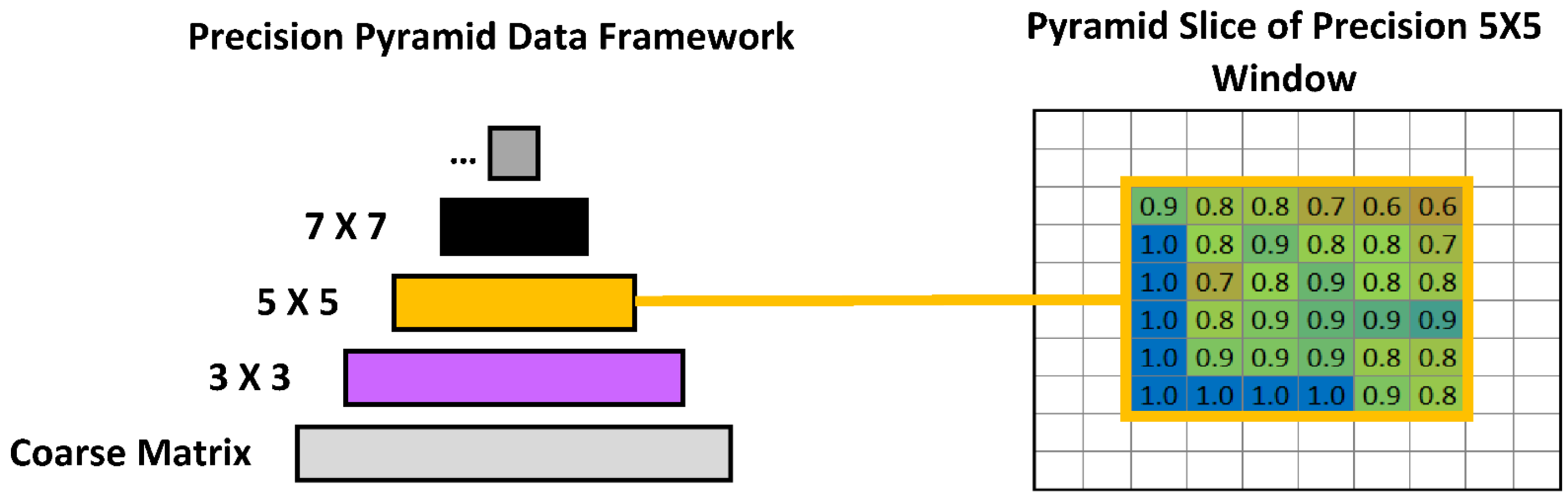
After creating the confusion matrix surfaces, a progressive focal window analysis transforms the coarse and fine uncertainty surfaces into a pyramid data framework. Three metrics are calculated within the focal windows: recall, precision, and F1. Starting with a three-by-three-pixel size, focal windows are moved across the entire surface and the desired metric is calculated for the pixels falling within the focal window. The analysis then iterates with increasingly large focal window sizes, and the calculated surfaces are stored in new layers of the pyramid data framework. The base layer of the pyramid contains the finest spatial resolution of the data (30 m). Figure 4 demonstrates this process, showing the original coarse matrix surface and three focal surfaces (or pyramid layers) that use a 3 × 3, 5 × 5, and a 7 × 7 window to calculate precision, recall and F1 metrics. The purple, orange, and black call-out lines demonstrate the size of the focal windows and the resulting pixel holding the precision value for the cells within that focal window.
As Figure 4 shows, when the focal window size grows an increasing amount of the edge is excluded because the focal window cannot extend beyond the limits of the original surface. While some researchers (e.g., [10]) strive to avoid edge bias due to the exclusion of border pixels, this study follows a different purpose, specifically to summarize the study area by building a hierarchy of progressive focal windows. The strategy effectively summarizes NWI and HGM agreement at progressively coarser levels of detail. Stacking the results surfaces for each size of the focal window, the filled cells create a pyramid shape with the original coarse matrix pixels lining the bottom and a single cell at the top that summarizes the entire study area (Figure 5). Figure 5 also demonstrates “slicing the pyramid”, which extracts a single layer of the pyramid to permit in-depth local analysis.
3. Results
3.1. Coarse Matrix—Wetlands Presence or Absence
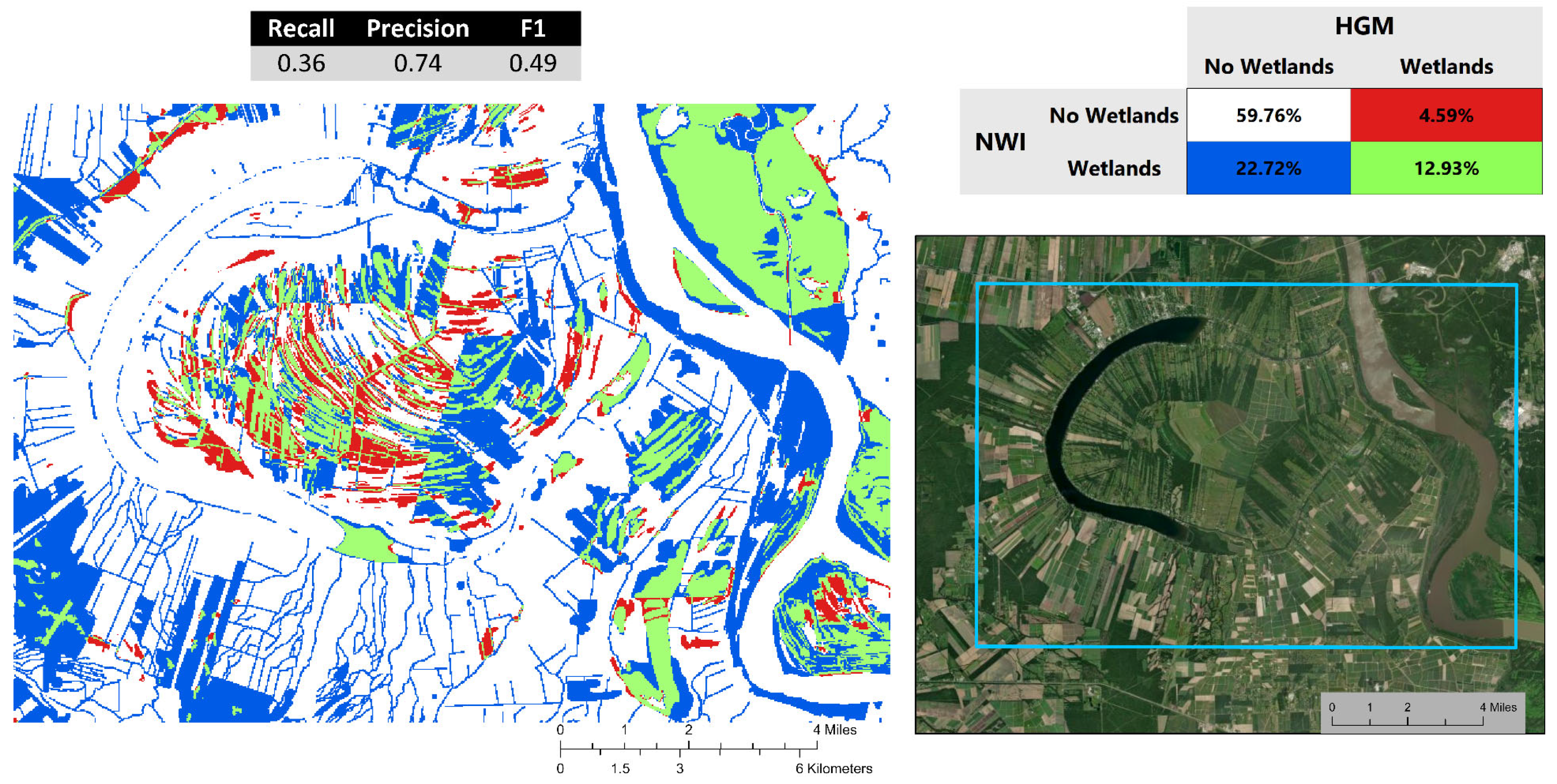
The coarse attribute uncertainty surface over the False River subarea is shown in Figure 6. Both HGM and NWI agree the majority (59.76%) of the subarea contains no wetlands. True positives (where HGM and NWI agree that wetlands are present) cover 12.93% of the subarea: the largest contiguous area is located to the east of the Mississippi with more isolated strips located in the central subarea. The second-largest classification is false negatives (22.72%) where the HGM detects no wetlands while NWI says wetlands are present. Large numbers of false negative pixels are located along the Mississippi River as well as in the southwest corner of the subset and the area around False River. False positives cover the smallest portion of the subarea (4.59%) and are located primarily around False River. Low recall and F1 values also indicate a large amount of disagreement.
3.2. Fine Matrix—Wetland Type
The fine attribute surface (Figure 7) gives a more in-depth view of wetlands’ attributes. A benefit of the fine matrix over the coarse matrix is that landscape features become more obvious. For example, the purple seen in Figure 7 indicates a lake is likely present just as blue indicates that a river or stream is present. The agricultural ditches seen in the center of the oxbow are more easily identifiable as well as in the lake in the southeast corner, neither of which is apparent in Figure 6.
Most of the NWI-classed riverine wetlands (light, medium and dark blue) within this area are false negatives (5.51%). These areas are situated next to the Mississippi and narrow channels in the southeast corner. It is likely that the channels are created by humans and are too small to be captured in the NHD dataset used to process the HGM dataset. Few lacustrine areas (purples) occur within the subarea with the majority outlining the oxbow and a contiguous patch in the southeast. Palustrine wetlands (greens) dominate the region and make up the majority of wetlands in this area. The highest recall, precision, and F1 values indicate the most agreement between the two datasets occurs in the areas classed as non-wetlands. The palustrine class has the second-highest scores. This is expected as there are few areas of riverine and lacustrine represented within this subarea and the HGM model does not detect smaller and isolated areas well.
3.3. Multiscale Analysis
A 200 × 200 pixel portion of the False River subarea (Figure 8) was used for the scale analysis. Recall, precision, and F1 pyramids were created for both coarse and fine attribute uncertainty surfaces and summarized for the subarea highlighted in yellow in the Figure. From these pyramids, and for simplicity of explanation, four layers (focal windows sized 5 × 5, 10 × 10, 15 × 15, and 20 × 20) are chosen from the coarse attribute pyramid to highlight cross-scale variations (Figure 9, Figure 10 and Figure 11). Summary statistics were calculated for each layer and a consolidated table is presented in Section 3.3.4.
3.3.1. Recall
Figure 9 shows slices from the Recall pyramid. Areas of high recall (blue shades) appear over the center and western part of the subarea as well as the northeastern corner. While the center region of layer five shows small areas of low recall values (red), by layer twenty they aggregate to show the center having the highest recall values in the study area. Low recall areas are focused along the edges at all four levels. These areas indicate higher levels of disagreement (false negatives). White regions mainly in layer 5 lack wetlands in HGM and NWI. As the window size increases, these regions gradually disappear as the focal window size exceeds areas without wetland pixels.
3.3.2. Precision
Slices from the precision pyramid are shown in Figure 10. Low precision values (red shades) appear in the center of layer five, but by layer ten and extending into layer twenty, two distinct low regions have emerged located in the northeast corner and south center. High-precision (blue) areas cluster along the eastern border and show as patches at all layers. Consistent precision patterns across all four focal window sizes imply that NWI shows more stable classes across the range of attribute scales.
3.3.3. F1
The F1 metric considers both precision and recall (Figure 11). High F1 (blue shades) indicate areas with the most agreement between the NWI and HGM datasets, while lower F1 (red shades) will indicate areas with the least agreement (false negatives and positives). While layer 5 seems to have a fragmented pattern, high F1 scores are consistent in the western border and patches of low F1 values emerge in layers 10, 15, and 20 along the edges. Most of the subarea has moderate F1 values (green shades).
When assessing agreement and disagreement across attribute scales, F1 appears to be the most informative metric as it considers both types of disagreement (false positives and negatives). Figure 12 shows this as it compares slices from Layer 20 of the precision, recall, and F1 pyramids. The single (blue) area that has a high F1 value can be seen in both the precision and recall slices. Areas such as the southeast corner that have high precision, but low recall are more tempered in the F1 layer with values closer to 0.5 (green). Similarly, the central region has lower precision values but higher recall. This shows why the F1 metric is valuable for isolating general areas of agreement and disagreement, as it accounts for both types of disagreement (false positives and negatives) and it is easier to see the combined spatial patterns of recall and precision. Recall and precision are more valuable when trying to isolate either false positives or false negatives and are more relevant when working with ground truth data.
While recall, precision, and F1 were all computed for the fine attribute resolution confusion matrices, F1 was found to be the most informative and therefore, only slices from the F1 pyramid are shown (Figure 13). Additionally, the fine attribute resolution confusion matrix is multivariate, so metrics are calculated individually for palustrine, riverine, and lacustrine classes. As palustrine dominates this portion of the study area, only the palustrine class is shown. The patterns of high and low F1 are similar to the coarse matrix F1 patterns shown in Figure 11 because palustrine takes up so much of the study area. However, the disagreement is more pronounced (deeper shades of red).
3.3.4. Consolidating and Comparing Metrics in the Pyramid Framework
Mean and standard deviation values were calculated for each pyramid layer. Table 2 reports the layer, the pixel size of the focal window used on that layer, and the number of windows needed for the surface. Additionally, Table 2 reports the mean and standard deviation (recall, precision, and F1) for each layer.
The mean and standard deviation are particularly useful in identifying patterns of attribute inconsistency. This can be seen in Figure 14 which plots the standard deviation and mean values for the first fifty layers in the coarse attribute F1, recall, and precision pyramids. The mean values drop (Box A) before reaching an equilibrium that is maintained at the top of the pyramid (Box C demonstrates this up to layer 49). Standard deviation values also drop for all three metrics, implying that the mean values better represent the central trend at coarse scales. After reaching an equilibrium in the metrics, further aggregation does not show new patterns of agreement/disagreement which is why the previous scale analysis selected layers 5, 10, 15 and 20. To demonstrate the equilibrium, the pyramid layers were calculated to the coarsest level, but in practice one needs to calculate the pyramid for layers prior to the equilibrium. A plot such as shown in Figure 14 may provide wetlands managers with an easy indication of the limits to usable resolution, showing that larger focal windows will obscure rather than highlight areas requiring further attention.
The magnitude of the initial drop depends in part on the proportion of true positives, false positives, and false negatives. A study area (such as False River) with more true positives (24.68%) than false negatives (23.68%) and false positives (18.55%) will not have as steep of an initial drop in the means as a study area with fewer true positives. A greater number of true positives (more agreement between classification systems) raises the recall, precision, and F1 means closer to 1.00 and as the pyramid summarizes more of the study area the larger number of true positives will cause the means to approach this maximum. The spread of the means also depends on the range of true positives, false positives, and false negatives. The False River mean values seen in Figure 14 are not dispersed because the study area has balanced levels of true positives, false negatives, and false positives. If False River had a much larger proportion of false positives and a low proportion of false negatives, the spread of the means would increase as the precision means would be much lower than the recall means.
4. Discussion
This research undertakes a multi-scale analysis of wetlands classification for a study area in Louisiana, where uncertainty is defined by disagreement (inconsistency) between independently compiled databases of similar credibility. Wetlands provide an example of what Fisher [36] calls “poorly defined objects” due to vagueness and ambiguity. These landscape features are considered vague due to difficulties in delimiting spatial extent. They are considered ambiguous due to inconsistent class definitions across databases. The two characteristics create special challenges for wetlands monitoring and management, as well as for error reporting to meet the Global Biodiversity Framework targets 1 and 2 [5]. Both reasons make wetlands an excellent data source to utilize in an analysis of classification uncertainty.
An additional complication in wetlands management is a frequent need for comprehensive field checking that could establish true and false wetland presence and type on the ground. Often a lack of field checking is due to pragmatic reasons (limited staff, resources, hydrological regime changes over time, or an expansive study area). Current imagery might assist in determining wetlands but is not always available for a specified time period or across the entire extent of managed areas. Complications with field checking can happen in study areas that are hard to access physically, have anthropogenic disruption, or other reasons. In the research reported here, imagery for the study area was not available for the same years for NWI and HGM data.
The remainder of the discussion addresses key points in the methods, results, and interpretations.
4.1. Evaluating Differences between Independently Compiled Data Classification Systems
Comber et al. [37] discuss variations that technical advances, data collection specifications, and mandates invariably introduce in digital data products representing the same landscape features. The Cowardin system was established as a national classification system to track wetland growth or retreat [21]. The HGM classification system reflects functional ecological characteristics that affect water storage and volume [23]. The pre-processing required to align the two classification systems (specifically for palustrine and riverine wetlands classes) was also described, reflecting concerns expressed by Comber et al. [36] that assumptions of database compatibility can interfere with uncertainty assessment. For example, the two classification systems treat open water in different ways, with one system using a unique category and the other merging it with other wetlands classes. Open water was eliminated from the analysis in order to avoid distorting the proportions of the study area in the comparison. One contribution of the work reported here is to demonstrate the importance of addressing classification alignment prior to beginning the assessment.
4.2. Advantages of Confusion Matrix Analysis to Highlight Classification Inconsistency
Another contribution of this work is to re-express confusion matrix analysis in the context of inconsistency or disagreement between two databases rather than as validation of empirical truth. In many cases of environmental uncertainty, ground truth is challenged or obstructed and, in these cases, the confusion matrix can provide an alternative assessment of uncertainty in the form of database agreement or disagreement. The traditional language used in confusion analysis can be adjusted using “agreement” and “disagreement” rather than true and false positives and negatives, carrying connotations that might be misleading for assessing inconsistency between two databases. The research also demonstrates that confusion analysis can be extended beyond binary classification to examine finer levels of attribute accuracy, in this study, categories of wetlands type.
In terms of wetlands presence overall, what is seen in both the coarse and fine matrices is influenced most likely by disturbance. Much of this area has been altered by agriculture. Plots of agricultural land can be seen in areal imagery such as the locator map in Figure 7. In addition to disturbance in this area, there is also a temporal difference between the NWI and HGM databases. The NWI data were collected in the 1970s and 1980s and the HGM data more recently. False negatives (off-diagonal percentages in Figure 2 and Figure 6) could indicate areas that were once wetlands (classed in the older NWI) but were destroyed and not classed in the newer HGM.
The fine attribute matrices tend to highlight landscape features, for example, the lacustrine and riverine wetlands in Figure 7 show probable locations of lakes and rivers, whether classified as such by one data classification or both. Smaller anthropogenic features such as agricultural ditches are also more prominent in the fine attribution, while they are not evident in the coarse attribution shown in Figure 6. In the finer matrix, the highest percentages of Recall, Precision and F1 scores are ascribed to areas classed as non-wetlands, with more disagreement earning lower scores. This offers insight into differences in how the two classification systems treat specific landscape features as well as which of the three confusion metrics is most informative. Findings in this study show that the F1 scores appear most informative about wetlands misclassification at both coarse and fine attribute scales.
In general, disturbance and temporal differences impact the patterns of disagreement. A data manager could utilize this information to update the datasets in areas with substantial amounts of disagreement such as in the center of False River. Being able to visualize areas of high disagreement can potentially save time and resources by allowing data managers to focus on specific areas within their monitored regions.
4.3. Benefits of the Pyramid Framework in Analyzing Confusion Matrix Metrics
One contribution of the paper is to demonstrate how patterns of uncertainty can be examined and quantified spatially and within levels of attribute categorization, in a method that links spatial with attribute levels of detail. This is accomplished using a pyramid framework to display discrepancies in wetlands attributes (presence or absence and type). The pyramid data framework allows multi-scale summary statistics to be stored in a single unified framework that can then be visualized and sliced to extract representations at individual levels of detail. Lower levels of the pyramid summarize local consistency while higher levels of the pyramid summarize more global patterns. The pyramid also shows the usable limits of resolution for analyzing data, as higher layers of the pyramid will eventually become too aggregated to offer additional local insights.
The analytical power of the pyramid framework as a container for multiscale data provides a ready method to provide focus in a large area of analysis. Patches of database agreement and disagreement become apparent as one travels through the layers of the pyramid. The pyramid data framework is an especially useful tool that allows one to assess confusion metrics at multiple scales. This is especially true for the F1 metric that considers both types of disagreement (in conventional confusion matrix analysis, false negatives, and false positives).
Calculating recall, precision, and F1 metrics at multiple focal window sizes is useful in finding not only local patterns but also generalized global patterns that smooth outliers. For example, inconsistency due to fragmentation is more apparent at a local scale, while overall data accuracy issues become more apparent at a global scale. Additional tools such as summary statistics can be calculated for each pyramid layer allowing one to easily compare the data at various levels of aggregation and see which levels are informative. What results is a way to visualize the attribute classification and determine how inconsistency patterns might vary across spatial and attribute scales.
The choice of source data’s spatial resolution will constrain the landscape patterns that are available for analysis. For example, in this study, the smaller stream channels, canals and agricultural ditches in the False River subarea are not resolved in the NHD data used to process the HGM data. No matter how fine the source data resolution, features too small to be detected at that resolution will be missed in the comparison. As the pyramid aggregates data by means of progressive focal windows, localized details are transformed into more global patterns. At a certain level of aggregation, global details and summary statistics will reach equilibrium and cease to change.
How many layers in the pyramid must be aggregated before the means reach an equilibrium depends on the spatial pattern and fragmentation of the true positives, false positives, and false negatives as well as on the size of the focal windows. Means and standard deviations for all three confusion matrix metrics are plotted for the first 50 layers of the pyramid in Figure 14. The layers where the means reach equilibrium are visually apparent. Spatial patterns of the wetlands inconsistencies can impact this summary. For example, if there are large areas of true positives and false negatives it will take a larger focal window for those areas to be aggregated. With more fragmented inconsistency patterns, the focal window does not need to be as large before patterns begin to cluster. If the areas of true positives and false positives are isolated, the focal window will need to be larger before those areas can affect the precision value. If large continuous patches of false positives (disagreement) are distant from true positives (agreement), the precision mean will require more layers in the pyramid (and larger focal windows) to summarize this pattern.
Figure 14 can be interpreted as having a few large, isolated clusters of values that are apparent both by looking at the black ticks in area B and by looking at the coarse matrix pattern in Figure 8. All three ticks occur before layer ten, a lower layer of the pyramid. Users can interpret this as an inconsistency surface being evenly dispersed. The spread of the standard deviation values reinforces this interpretation. If patches of disagreement were clustered for example, the Recall standard deviation would be higher, and more layers would be required for the recall mean reach equilibrium because larger focal windows would be required to smooth over a large cluster.
In summary, plotting the mean and standard deviation recall, precision, and F1 values lends important insights into the study areas. The spread of means, rate of their initial decrease, and point at which they level off give insight into the composition and spatial patterns of the study area. Means that have a quick and shallow decrease with little spread indicate the study area has more true positives (agreement that wetlands exist) than true and false negatives (disagreement about wetland presence). A shallow decrease without spread also indicates that patches of similar attribute agreement or disagreement occur in small clusters that are spatially proximal. Standard deviations also give insight into the spatial pattern of the study areas. Higher standard deviations indicate more extreme high and low values for that metric within the study area. Extremely high and low recall and precision standard deviation values will occur where there is a large amount of disagreement and areas where agreement occurs lie in isolated patches. Visualizing inconsistency at multiple scales shows where the disagreement is most extreme. The pyramid slices can identify areas of high inconsistency within a single focal layer.
5. Conclusions
This research assesses categorical uncertainty in two attribute levels of wetland classification and creates visualization tools to guide the analysis of spatial uncertainty patterns over several scales. A novel variant of confusion matrix analysis compares the Cowardin and Hydrogeomorphic wetland classification systems. Algorithms were developed to identify areas and types of misclassification for binary and multivariate categories. Code implementing these algorithms as well as wetlands test data used in the case study is available in the public domain (see Data Availability Statement below). The specific focus on uncertainty in the paper refers to categorical consistency, that is, agreement between the two classification systems, rather than comparing observed data to ground truth. To the authors’ knowledge, no previously published research utilizes confusion matrix analysis to assess categorical accuracy using empirical data, either at a single scale or within a hierarchy of scales.
The work reported here carries several limitations. One is a temporal difference between the NWI and HGM data. The NWI data in this region were collected in the 1970s and 1980s with a small portion collected in the 2010s, intermixing field checking with image and geospatial analysis. However, the data used to create the HGM database was collected after the 2000s. It is likely that temporal uncertainty is contributing to some database disagreement. Wetlands that existed when the NWI was created but destroyed in later years would appear as false negatives: NWI would class the area as wetlands while the HGM would not. Conversely, the HGM may detect where wetlands once existed. Drained soils may still be classed as hydric and some areas with hydric soils will not be classified as wetlands by HGM but not by NWI [38,39]. The temporal disagreement especially shows itself in disturbed areas such as the area of agricultural development around False River.
A second limitation Is that several assumptions were made in generating the HGM dataset that may not be true in every geographic case. For example, the assumption that soils classed as hydric are always wetlands is not always correct, nor that wetlands adjacent to rivers and lakes are always riverine and lacustrine, respectively. However, the purpose of this analysis is to demonstrate a method and data framework to explore multi-scale patterns of attribute accuracy, rather than to establish a spatially precise model of wetlands in the False River oxbow.
Another limitation of this work is its examination of only a single study area. Wetlands emerge in a variety of ways in different landscape conditions, and their persistence is impacted by factors including precipitation, soils and vegetation, topography, and human disruption. Examination of wetlands in a variety of conditions will inform and advance understanding of how patterns of uncertainty manifest across spatial and attribute scales, and whether the patterns are stable or variant. Additional study areas will also provide guidance on the efficacy of the confusion matrix analysis and of the pyramid data framework for studying uncertainty across scales. This forms an area of ongoing research, and a study area in the Pacific Northwest is under investigation [40].
The tools created in this research can help land managers, regulators, researchers, and conservationists by allowing them to focus time and resources on wetland areas of highest uncertainty, as they may need updated data for specialized management and monitoring. Visualizations of attribute uncertainty can shorten analysis and facilitate decision-making for areas when time, funding or labor is short. These tools offer a direct advantage for reporting progress and errors in quantitative ways, following the IUCN’s resolutions to advance the Global Biodiversity Framework. Additionally, the temporal difference in the data and the inherent difference between the hydrogeomorphic (HGM) and Cowardin classification systems can offer insight into historic wetlands patterns and impacts of disturbance or disruption. Furthermore, the methodologies used in this research are not limited to wetlands, and others working with categorical or classified geospatial data could apply these methodologies to their own work. In natural and social science domains, our methods are directly applicable to compare for example databases or classification systems reporting land cover vegetation, land parcel ownership (public, private, governmental), or social categories such as race or ethnicity at province, state, county or local levels.
Author Contributions
Conceptualization, Barbara P. Buttenfield and Kate Carlson; methodology, Barbara P. Buttenfield and Yi Qiang; software, Kate Carlson; validation, Kate Carlson; formal analysis, Kate Carlson and Barbara P. Buttenfield; investigation, Kate Carlson; data curation, Kate Carlson; writing—original draft preparation, Kate Carlson; writing—review and editing, Barbara P. Buttenfield and Yi Qiang; visualization, Kate Carlson; supervision, Barbara P. Buttenfield; project administration, Yi Qiang; funding acquisition, Yi Qiang and Barbara P. Buttenfield. All authors have read and agreed to the published version of the manuscript.
Funding
This material is based upon work supported by the National Science Foundation under Grant No. 2102019, “Cross-Scale Spatiotemporal Modeling Using an Integrated Data Framework”, a collaboration among researchers at the University of South Florida—Tampa, University of Colorado—Boulder, and University of Hawaii—Manoa. Any opinions, findings, and conclusions or recommendations expressed in this material are those of the author(s) and do not necessarily reflect the views of the National Science Foundation.
Data Availability Statement
All data is available in the public domain. Code is available as well as a tutorial and sample data on the CroScalar website (https://croscalar.github.io/index.html) or at https://spot.colorado.edu/~babs/croscalar/. Both links accessed 18 March 2024.
Acknowledgments
This work represents a portion of Kate Carlson’s Masters thesis [40] at the University of Colorado—Boulder, supervised by Barbara P. Buttenfield.
Conflicts of Interest
The authors declare no conflicts of interest.
References
- Couclelis, H. The Certainty of Uncertainty: GIS and the Limits of Geographic Knowledge. Trans. GIS 2003, 7, 165–175. [Google Scholar] [CrossRef]
- Hope, S.; Hunter, G.J. Testing the effects of positional uncertainty on spatial decision-making. Int. J. Geogr. Inf. Sci. 2007, 21, 645–665. [Google Scholar] [CrossRef]
- MacEachren, A.M. Visualizing Uncertain Information. Cartogr. Perspect. 1992, 13, 10–19. [Google Scholar] [CrossRef]
- Mason, J.S.; Klippel, A.; Bleisch, S.; Slingsby, A.; Deitrick, S. Special issue introduction: Approaching spatial uncertainty visualization to support reasoning and decision making. Spat. Cogn. Comput. 2016, 16, 97–105. [Google Scholar] [CrossRef]
- International Union of Conservation of Nature (IUCN). Contributing to the Kunming-Montreal Global Biodiversity Framework: Nature 2030, IUCN Resolutions and Conservation Tools; IUCN International Policy Centre: Gland, Switzerland, 2023; Available online: https://www.iucn.org/sites/default/files/2023-10/information-note-iucn-and-the-gbf.pdf (accessed on 14 March 2024).
- Usery, E.L.; Finn, M.P.; Cox, J.D.; Beard, T.; Ruhl, S.; Bearden, M. Projecting Global Datasets to Achieve Equal Areas. Cartogr. Geogr. Inf. Sci. 2003, 30, 69–79. [Google Scholar] [CrossRef]
- Tobler, W.R. A Transformational View of Cartography. Am. Cartogr. 1979, 6, 101–106. [Google Scholar] [CrossRef]
- Visvalingham, M.; Whyatt, J.D. Line Generalization by Repeated Elimination of Points. Cartogr. J. 1993, 30, 46–51. [Google Scholar] [CrossRef]
- Kronenfeld, B.J.; Stanislawski, L.V.; Buttenfield, B.P.; Brockmeyer, T. Simplification of Polylines by Segment Collapse: Minimizing Areal Displacement While Preserving Area. Int. J. Cartogr. 2019, 6, 22–46. [Google Scholar] [CrossRef]
- Radtke, P.J.; Burkhardt, H.E. A Comparison of Methods for Edge Bias Compensation. Can. J. For. Res. 2011, 28, 942–945. [Google Scholar] [CrossRef]
- Jenks, G.F. Optimal Data Classification for Choropleth Maps; Occasional Paper #2; Department of Geography, University of Kansas: Lawrence, KS, USA, 1977. [Google Scholar]
- Slocum, T.A.; McMaster, R.B.; Kessler, F.C.; Howard, H.H. Thematic Cartography and Geovisualization, 4th ed.; CRC Press: Boca Raton, FL, USA, 2022. [Google Scholar] [CrossRef]
- Millennium Ecosystem Assessment. Ecosystems and Human Well-Being: Wetlands and Water; World Resources Institute: Washington, DC, USA, 2005; Available online: https://www.unep.org/resources/report/ecosystems-and-human-well-being-wetlands-and-water-synthesis (accessed on 14 March 2024).
- Smith, R.D.; Ammann, A.; Bartoldus, C.; Brinson, M.M. An Approach for Assessing Wetland Functions Using Hydrogeomorphic Classification, Reference Wetlands, and Functional Indices; Technical Report WRP-DE-9; U.S Army Corps of Engineers, Wetlands Research Program: Washington, DC, USA, 1995; Available online: https://www.semanticscholar.org/paper/An-approach-for-assessing-wetland-functions-using-%3B-Smith-Ammann/63aae965cd55159cf32861d1d4bbda0e45e0449f (accessed on 14 March 2024).
- McCauley, L.A.; Jenkins, D.G.; Quintana-Ascencio, P.F. Isolated Wetland Loss and Degradation Over Two Decades in an Increasingly Urbanized Landscape. Wetlands 2013, 33, 117–127. [Google Scholar] [CrossRef]
- Tiner, R.W. Assessing cumulative loss of wetland functions in the Nanticoke River watershed using enhanced National Wetlands Inventory data. Wetlands 2005, 25, 405–419. [Google Scholar] [CrossRef]
- Dahl, T.E. Wetlands Losses in the United States 1780’s to 1980’s; U.S. Department of the Interior, Fish and Wildlife Service: Washington, DC, USA, 1990. Available online: https://www.fws.gov/media/wetland-losses-united-states-1780s-1980s (accessed on 14 March 2024).
- Coastal Protection and Restoration Authority of Louisiana. Louisiana’s Comprehensive Master Plan for a Sustainable Coast; Coastal Protection and Restoration Authority of Louisiana: Baton Rouge, LA, USA, 2017. Available online: http://coastal.la.gov/wp-content/uploads/2017/04/2017-Coastal-Master-Plan_Web-Single-Page_CFinal-with-Effective-Date-06092017.pdf (accessed on 14 March 2024).
- Laws, F. Swampbuster Rules Set Off 18-Year Court Battle; Delta Farm Press: Boone, IA, USA, 2020; Available online: https://www.farmprogress.com/farm-life/swampbuster-rules-set-off-18-year-court-battle (accessed on 14 March 2024).
- Dvorett, D.; Bidwell, J.; Davis, C.; DuBois, C. Developing a Hydrogeomorphic Wetland Inventory: Reclassifying National Wetlands Inventory Polygons in Geographic Information Systems. Wetlands 2012, 32, 83–93. [Google Scholar] [CrossRef]
- FGDC (Federal Geographic Data Committee). Classification of Wetlands and Deepwater Habitats of the United States (FGDC-STD-004-2013), 2nd ed.; Wetlands Subcommittee, Federal Geographic Data Committee and U.S. Fish and Wildlife Service: Reston, VA, USA, 2013. Available online: https://www.fws.gov/sites/default/files/documents/Classification-of-Wetlands-and-Deepwater-Habitats-of-the-United-States-2013.pdf (accessed on 14 March 2024).
- EPA (U.S. Environmental Protection Agency). Methods for Evaluating Wetland Condition: Wetlands Classification; EPA-822-R-02-017; EPA Office of Water: Washington, DC, USA, 2002. Available online: https://www.epa.gov/sites/default/files/documents/wetlands_7classification.pdf (accessed on 14 March 2024).
- Brinson, M.M. A Hydrogeomorphic Classification for Wetlands; Technical Report WRP-DE-4; U.S. Army Engineer Waterways Experiment Station, Wetlands Research Program: Vicksburg, MS, USA, 1993; Available online: https://wetlands.el.erdc.dren.mil/pdfs/wrpde4.pdf (accessed on 14 March 2024).
- FS077-99; SDTS, (Spatial Data Transfer Standard). U.S. Geological Survey: Washington, DC, USA, 1999. [CrossRef]
- Smith, R.D.; Noble, C.V.; Berkowitz, J.F. Hydrogeomorphic (HGM) Approach to Assessing Wetland Functions: Guidelines for Developing Guidebooks (Version 2); Report # ERDC/EL TR-13-11; U.S. Army Engineer Research and Development Center Wetlands Regulatory Assistance Program: Vicksburg, MS, USA, 2013; Available online: https://www.semanticscholar.org/paper/Hydrogeomorphic-HGM-Approach-to-Assessing-Wetland-Smith-Noble/719ffd937c00bb8ae9c526f8a9a4abc60dad63de (accessed on 14 March 2024).
- ISO (International Organization for Standardization). Report 19115-1:2014/Amd 2:2020 Geographic Information–Metadata; International Organization for Standardization: Geneva, Switzerland, 2020; Available online: https://www.iso.org/standard/80275.html (accessed on 14 March 2024).
- FGDC (Federal Geographic Data Committee). Content Standard for Digital Geospatial Metadata (FGDC-STD-001-1998); Federal Geographic Data Committee: Washington, DC, USA, 1998. Available online: https://www.fgdc.gov/standards/projects/metadata/base-metadata/v2_0698.pdf (accessed on 14 March 2024).
- Tobler, W.R.T. Measuring Spatial Resolution. In Proceedings of the International Workshop on Land Use and Remote Sensing, Beijing, China, 25–28 January 1987; Available online: https://www.researchgate.net/publication/291877360_Measuring_spatial_resolution (accessed on 14 March 2024).
- Cedfeldt, P.T.; Watzin, M.C.; Richardson, B.D. Using GIS to Identify Functionally Significant Wetlands in the Northeastern United States. Environ. Manag. 2000, 26, 13–24. [Google Scholar] [CrossRef] [PubMed]
- Adamus, P.; Christy, J.; Jones, A.; McCune, M.; Bauer, J. A Geodatabase and Digital Characterization of Wetlands Mapped in the Willamette Valley with Particular Reference to Prediction of Their Hydrogeomorphic (HGM) Class; U.S. Environmental Protection Agency Region: Portland, OR, USA, 2010; Volume 10. [Google Scholar] [CrossRef]
- Van Deventer, H.; Nel, J.; Mbona, N.; Job, N.; Ewart-Smith, J.; Snaddon, K.; Maherry, A. Desktop classification of inland wetlands for systematic conservation planning in data-scarce countries: Mapping wetland ecosystem types, disturbance indices and threatened species associations at country-wide scale. Aquat. Conserv. Mar. Freshw. Ecosyst. 2016, 26, 57–75. [Google Scholar] [CrossRef]
- Rivers-Moore, N.A.; Kotze, D.C.; Job, N.; Mohanlal, S. Prediction of Wetland Hydrogeomorphic Type Using Morphometrics and Landscape Characteristics. Front. Environ. Sci. 2020, 8, 58. [Google Scholar] [CrossRef]
- Tiner, R.W. Keys to Landscape Position and Landform Descriptors for U.S. Wetlands; U.S. Fish and Wildlife Service, National Wetlands Inventory Program, Northeast Region: Hadley, MA, USA, 1997. [Google Scholar]
- Powers, D.M.W. Evaluation: From Precision, Recall and F-Factor to ROC, Informedness, Markedness and Correlation. arXiv 2010, arXiv:2010.16061. [Google Scholar] [CrossRef]
- Hand, D.; Christen, P. A note on using the F-measure for evaluating record linkage algorithms. Stat. Comput. 2018, 28, 539–547. [Google Scholar] [CrossRef]
- Fisher, P.F. Models of uncertainty in spatial data. In Geographical Information Systems: Principles, Techniques, Management and Applications, 2nd ed.; Longley, P.A., Goodchild, M.F., Maguire, D.J., Rhind, D.W., Eds.; Wiley: London, UK, 2005; pp. 191–205. [Google Scholar]
- Comber, A.J.; Fisher, P.F.; Harvey, F.; Gahegan, M.; Wadsworth, R. Using Metadata to Link Uncertainty and Data Quality Assessments. In Progress in Spatial Data Handling; Riedl, A., Kainz, W., Elmes, G.A., Eds.; Springer: Berlin/Heidelberg, Germany, 2006; pp. 279–292. [Google Scholar] [CrossRef]
- National Standards and Support Team. Technical Procedures for Conducting Status and Trends of the Nation’s Wetlands; Version 2; U.S. Fish and Wildlife Service: Washington, DC, USA, 2017. Available online: https://www.govinfo.gov/content/pkg/GOVPUB-I49-PURL-gpo145058/pdf/GOVPUB-I49-PURL-gpo145058.pdf (accessed on 18 March 2024).
- NRCS (U.S. Natural Resources Conservation Service). Field Indicators of Hydric Soils in the United States; A Guide for Identifying and Delineating Hydric Soils; Version 8.2; U.S. Department of Agriculture, in cooperation with the National Technical Committee for Hydric Soils: Washington, DC, USA, 2018. Available online: https://www.nrcs.usda.gov/resources/guides-and-instructions/field-indicators-of-hydric-soils (accessed on 18 March 2024).
- Carlson, K. Wetland Classification Accuracy and Scale: Visualizing Uncertainty Metrics Across Multiple Resolutions. Master’s Thesis, Department of Geography, University of Colorado–Boulder, Boulder, CO, USA, 2021. [Google Scholar]
Figure 1.
The red outline shows the 2000 square mile study area located in Louisiana. The blue outline shows the subarea focusing on the False River oxbow lake. (A) shows the study area outlined in red. (B) shows an inset used for the multiscale analysis, around the Flse River oxbow.
Figure 1.
The red outline shows the 2000 square mile study area located in Louisiana. The blue outline shows the subarea focusing on the False River oxbow lake. (A) shows the study area outlined in red. (B) shows an inset used for the multiscale analysis, around the Flse River oxbow.

Figure 2.
Key for the coarse attribute uncertainty surface. The matrix compares the presence versus the absence of wetlands in the NWI and HGM data sets. True negatives (white) and positives (green) indicate areas where the data sets agree, while false negatives (blue) and positives (red) show areas of disagreement.

Figure 3.
Key for the fine attribute uncertainty surface. This key compares not only the presence versus the absence of wetlands, but also the agreement of the specific wetland classification (riverine, lacustrine, and palustrine).
Figure 3.
Key for the fine attribute uncertainty surface. This key compares not only the presence versus the absence of wetlands, but also the agreement of the specific wetland classification (riverine, lacustrine, and palustrine).

Figure 4.
Shows an example of three differently sized focal windows (3 × 3, 5 × 5, and 7 × 7) used to calculate precision for the same coarse matrix surface. It is important to note that precision does not involve true or false negatives (blue and white), only true positives and false positives (green and red). An example 3 × 3 window is shown to demonstrate how a hypothetical precision value of 0.57 is derived from a coarse matrix surface. The precision value calculated for a focal window is stored in the center pixel as shown for each window size. The focal window is moved exhaustively across the entire coarse matrix surface. The purple, orange, and black dashed callout lines show where the focal windows begin and their corresponding calculated precision values stored in the 3 × 3, 5 × 5, and 7 × 7 focal window surfaces.

Figure 5.
Shows an example of the hierarchical pyramid data framework created from the focal window analysis shown in Figure 4. which uses precision as the metric. The base layer of the pyramid is the original coarse matrix. Subsequent pyramid layers store the calculated surfaces from the focal window analysis. The purple, orange, and black layers contain the calculated 3 × 3, 5 × 5, and 7 × 7 precision focal window surfaces shown in Figure 4. Additional layers with larger focal windows can be calculated and inserted into higher layers of the pyramid but are not shown. Slicing the pyramid extracts one of the pyramid layers for more local analysis. A slice of the third layer which contains the 5 × 5 pixel focal window is shown.

Figure 6.
Coarse attribute uncertainty surface over the False River subarea. Recall, precision, and F1 scores are reported for the subarea. The blue frame bounds the mapped area on a satellite image.
Figure 6.
Coarse attribute uncertainty surface over the False River subarea. Recall, precision, and F1 scores are reported for the subarea. The blue frame bounds the mapped area on a satellite image.

Figure 7.
Fine attribute uncertainty surface over the False River subarea. Recall, Precision, and F1 are reported for each of the wetland classes present in the subarea. The blue frame bounds the mapped area in a satellite image.
Figure 7.
Fine attribute uncertainty surface over the False River subarea. Recall, Precision, and F1 are reported for each of the wetland classes present in the subarea. The blue frame bounds the mapped area in a satellite image.

Figure 8.
The 200 × 200 pixel portion of the False River subarea used for the multiscale analysis. The coarse attribute resolution confusion matrix is shown along with the recall, precision, and F1 values calculated at the finest pyramid level (3 × 3 focal window) for this subarea. The locator map shows the 200 × 200 pixel area outlined in yellow within the False River subarea outlined in blue.

Figure 9.
Four slices from the coarse attribute surface recall pyramid. Layer number indicates the height in the pyramid and window number indicates the size of the square focal window used in that layer.
Figure 9.
Four slices from the coarse attribute surface recall pyramid. Layer number indicates the height in the pyramid and window number indicates the size of the square focal window used in that layer.

Figure 10.
Four slices from the coarse attribute surface precision pyramid. Layer number indicates the height in the pyramid and window number indicates the size of the square focal window used in that layer.
Figure 10.
Four slices from the coarse attribute surface precision pyramid. Layer number indicates the height in the pyramid and window number indicates the size of the square focal window used in that layer.

Figure 11.
Four slices from the coarse attribute surface F1 pyramid. Layer number indicates the height in the pyramid and window number indicates the size of the square focal window used in that layer.
Figure 11.
Four slices from the coarse attribute surface F1 pyramid. Layer number indicates the height in the pyramid and window number indicates the size of the square focal window used in that layer.

Figure 12.
Layer twenty from the coarse attribute resolution precision, recall, and F1 pyramids. Areas that have both high recall and precision, as well as areas with low recall and precision, can be seen in the F1 slices.
Figure 12.
Layer twenty from the coarse attribute resolution precision, recall, and F1 pyramids. Areas that have both high recall and precision, as well as areas with low recall and precision, can be seen in the F1 slices.

Figure 13.
Four slices from the fine attribute pyramid showing F1 scores calculated for the palustrine class. Layer number indicates the height in the pyramid and window number indicates the size of the square focal window used in that layer.
Figure 13.
Four slices from the fine attribute pyramid showing F1 scores calculated for the palustrine class. Layer number indicates the height in the pyramid and window number indicates the size of the square focal window used in that layer.

Figure 14.
These charts plot the mean and standard deviation F1, precision, and recall scores for the first fifty layers of the coarse attribute pyramid. Box A is around the initial fall in mean Precision, Recall, and F1 values in the first few layers. B indicates the three black dashes on the mean lines that indicate where the means stop their initial descent. Box C is the portion of the graph where the means have reached an equilibrium and do not drastically change.


Table 1.
Data Layers.
| Data Layer | Source | Resolution | Years Collected |
|---|---|---|---|
| Land Cover | NLCD-USGS | 30 m | 2016 |
| Wetlands | NWI-FWS | 1:65,000 | 1970s, 1980s, 2010s |
| Elevation | USGS | 30 m | 2016 |
| Hydric Soils | SSURGO-NRCS | 1:20,000 | 2000s–2019 |
| Hydrography | NHD-USGS | 1:24,000 | 2000s–2010 |
Table 2.
Coarse Attribute Confusion Matrix Multiscale Analysis Metrics.
| Recall | Precision | F1 | ||||||
|---|---|---|---|---|---|---|---|---|
| Layer | Window Size | # of Windows | Std Dev | Mean | Std Dev | Mean | Std Dev | Mean |
| 5 | 7 | 37,636 | 0.32 | 0.64 | 0.30 | 0.66 | 0.24 | 0.54 |
| 10 | 17 | 33,856 | 0.28 | 0.58 | 0.27 | 0.59 | 0.20 | 0.50 |
| 15 | 27 | 30,276 | 0.23 | 0.58 | 0.27 | 0.57 | 0.17 | 0.51 |
| 20 | 37 | 26,896 | 0.19 | 0.59 | 0.19 | 0.56 | 0.14 | 0.53 |
Disclaimer/Publisher’s Note: The statements, opinions and data contained in all publications are solely those of the individual author(s) and contributor(s) and not of MDPI and/or the editor(s). MDPI and/or the editor(s) disclaim responsibility for any injury to people or property resulting from any ideas, methods, instructions or products referred to in the content. |
© 2024 by the authors. Licensee MDPI, Basel, Switzerland. This article is an open access article distributed under the terms and conditions of the Creative Commons Attribution (CC BY) license (https://creativecommons.org/licenses/by/4.0/).
Share and Cite
MDPI and ACS Style
Carlson, K.; Buttenfield, B.P.; Qiang, Y. Wetland Classification, Attribute Accuracy, and Scale. ISPRS Int. J. Geo-Inf. 2024, 13, 103. https://0-doi-org.brum.beds.ac.uk/10.3390/ijgi13030103
AMA Style
Carlson K, Buttenfield BP, Qiang Y. Wetland Classification, Attribute Accuracy, and Scale. ISPRS International Journal of Geo-Information. 2024; 13(3):103. https://0-doi-org.brum.beds.ac.uk/10.3390/ijgi13030103
Chicago/Turabian StyleCarlson, Kate, Barbara P. Buttenfield, and Yi Qiang. 2024. "Wetland Classification, Attribute Accuracy, and Scale" ISPRS International Journal of Geo-Information 13, no. 3: 103. https://0-doi-org.brum.beds.ac.uk/10.3390/ijgi13030103
Note that from the first issue of 2016, this journal uses article numbers instead of page numbers. See further details here.