3-Dimensional Modeling and Simulation of the Cloud Based on Cellular Automata and Particle System

Abstract

The authors combine the cellular automata with particle system to realize the three-dimensional modeling and visualization of the cloud in the paper. First, we use the principle of particle systems to simulate the outline of the cloud; generate uniform particles in the bounding volumes of the cloud through random function; build the cloud particle system; and initialize the particle number, size, location and related properties. Then the principle of cellular automata system is adopted to deal with uniform particles simulated by the particle system to make it conform to the rules set by the user, and calculate its continuous field density. We render the final cloud particles with a texture map and simulate the more realistic three-dimensional cloud. This method not only obtains the real effect in the simulation, but also improves the rendering performance.

1. Introduction

Clouds are a common atmospheric phenomenon. With the development of computer visualization technologies, computer simulation of clouds becomes possible. Researchers around the world have done a lot of research on this topic. The research results have been widely used in virtual battlefield simulations, flight simulations, natural environment building in games and animations. Particularly, the simulation of clouds in weather forecasting study is even more important. As one of the main weather information sources, satellite cloud images play a critical role in cloud simulation as original data sources. Currently, most primary meteorological departments use two-dimensional display technologies to display and process satellite cloud images. If the cloud images are displayed using three-dimensional simulation, the spatial distribution of clouds can be recovered. The contrast of clouds at different levels can be enhanced. Therefore, forecasters can analyze and judge typical weather phenomena, such as thunderstorms, low vortex, and frontal rain, more easily. Furthermore, the weather forecasting will be more precise [1]. Scholars around the world have carried out numerous studies and experiments on cloud modeling and obtained many effective cloud modeling algorithms. These algorithms can be divided into numerical simulation methods and modeling methods based on appearance.

In order to simulate large-scale clouds, in 2006, Dobashi et al. [2] solved the atmospheric fluid dynamics equations by mapping them to grids in the polar coordinates, achieving the simulation of earth-scale clouds. Recently, in order to improve the efficiency of cloud simulation, Wang et al. [3] divided the three-dimensional space into a one-dimensional space in the vertical direction and a two-dimensional space in the horizontal direction, transforming complex variables to constants. They used this simplified solution to implement the simulation of cumulus clouds and reduce the computational overhead. However, the amount of computation of solving atmospheric fluid dynamics equations is still large. Therefore, numerical simulation methods are rarely used in fast cloud simulation. The modeling methods based on appearance include the fractal geometry [4], metaball algorithm [5], and particle systems [6]. Nishita et al. [5] combined the metaball algorithm with the fractal algorithm to generate an irregular cloud which looks real with a flat bottom and an irregular top. Dobashi et al. [7] placed metaballs according to satellite cloud images. They finally implemented the cloud simulation by adjusting the radii and concentration of the metaballs. In 2008, Wang et al. [6] utilized the particle system to carry out their research. They controlled the upward motion of vapor particles by using an approximate numerical model to simulate physical factors. Meanwhile, the life cycle of a particle determines its cohesion time on the grid and its position change on the grid determines the phase change of the grid, thereby obtaining the cloud form data. In summary, these methods are simple and have smaller amount of computation. Based on the above analysis, a three-dimensional modeling algorithm based on the cellular automaton and particle system is proposed in this paper. In addition, corresponding dynamic simulation is carried out.

2. Simulating Uniform Cloud Particles Using the Particle System

2.1. Overview of the Particle System

The basic idea of the particle system is to assume that an object is composed of numerous simple-shape particles. Each particle has its own life cycle and the particle will experience four stages during its lifetime: “birth”, “motion”, “growth”, and “disappearance”. The motion characteristics of the object can be described by random processes. All particles move and change their shapes constantly, reflecting the internal nature and dynamics of the irregular object [8,9].

Figure 1 illustrates the flow chart of a closed particle system. First of all, a given number of particles are generated randomly in the three-dimensional space describing the shape of an object. Then each particle is given physical properties, such as the state, speed, position, color, and life cycle based on particle properties. Finally, according to the motion rules of the object, the dynamic property change equations of the particle are established. During the motion process of particles, we need to detect whether a particle’s lifetime exceeds a predetermined value. If yes, we should remove these particles and produce a number of new particles as needed. Finally, rendering and drawing operations are carried out on the three-dimensional model which is established using the particle system.

Whether the modeled object is solid, liquid, or gaseous, such as flame, clouds, smoke, etc., all of them can be simulated using the particle system. The particle system can effectively reflect the dynamic characteristics of fuzzy and irregular objects, such as clouds, fog, smoke, etc. Therefore, the particle system is a good graphics generation algorithm for simulating irregular and fuzzy objects.

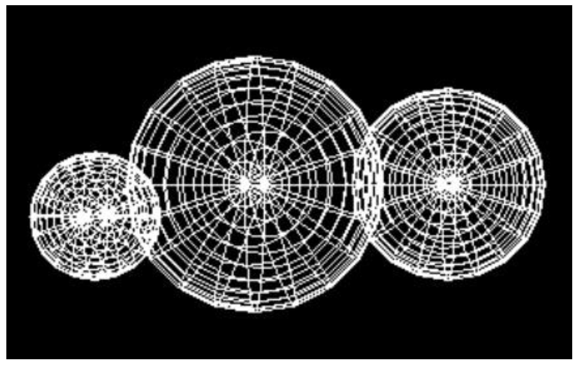
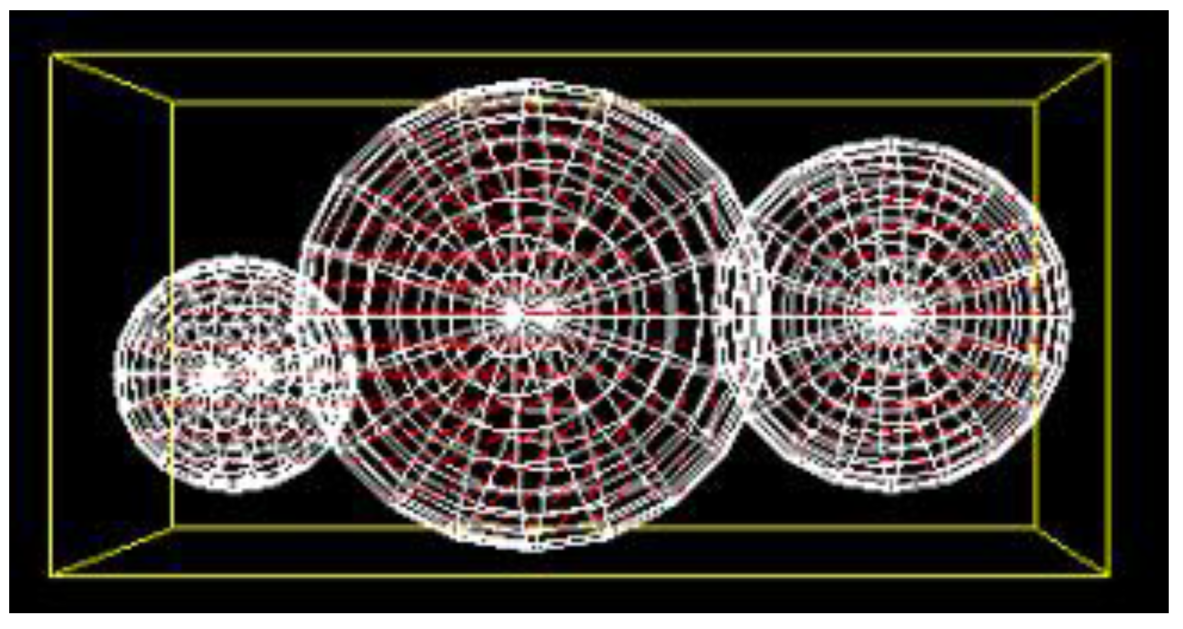
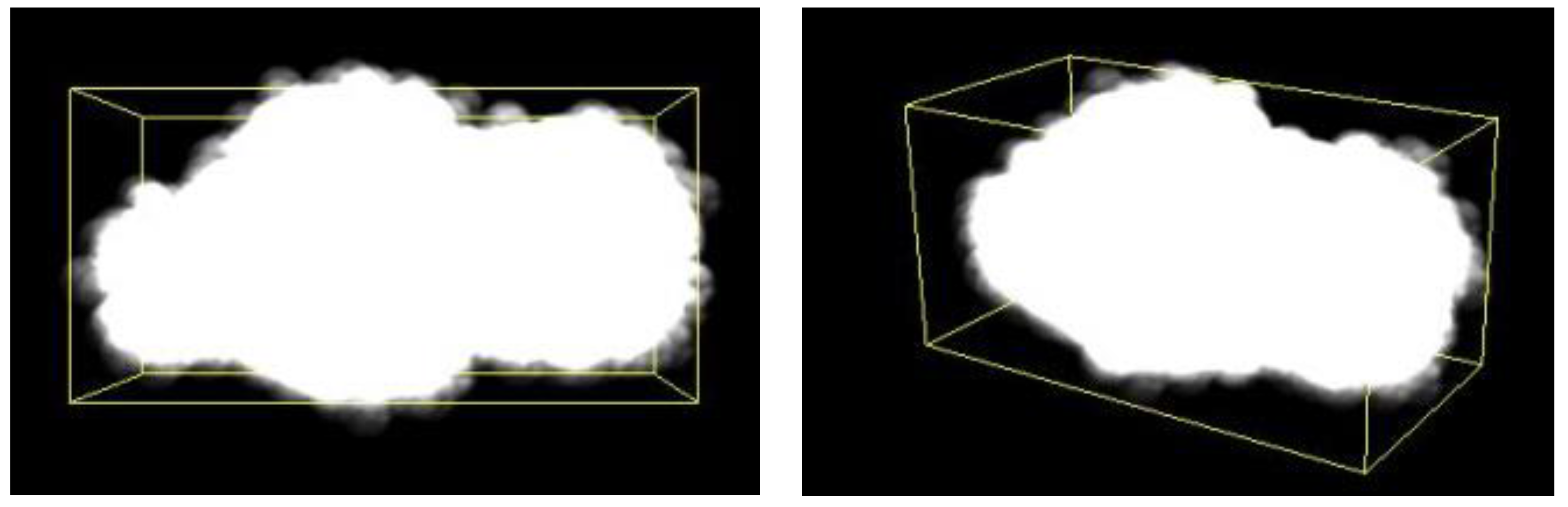
2.2. Using Spheres to Simulate the Cloud Contour

Each cloud looks like a quasi-sphere or an irregular sphere; therefore, we use spheres to simulate the cloud contour. A cloud with any shape can be formed using a large number of spheres of different sizes. For the sake of convenience, we use three spheres with different radii to form a cloud. As a result, only a few simple structures are needed to describe these three spheres. Figure 2 shows the cloud contour simulated using different balls.

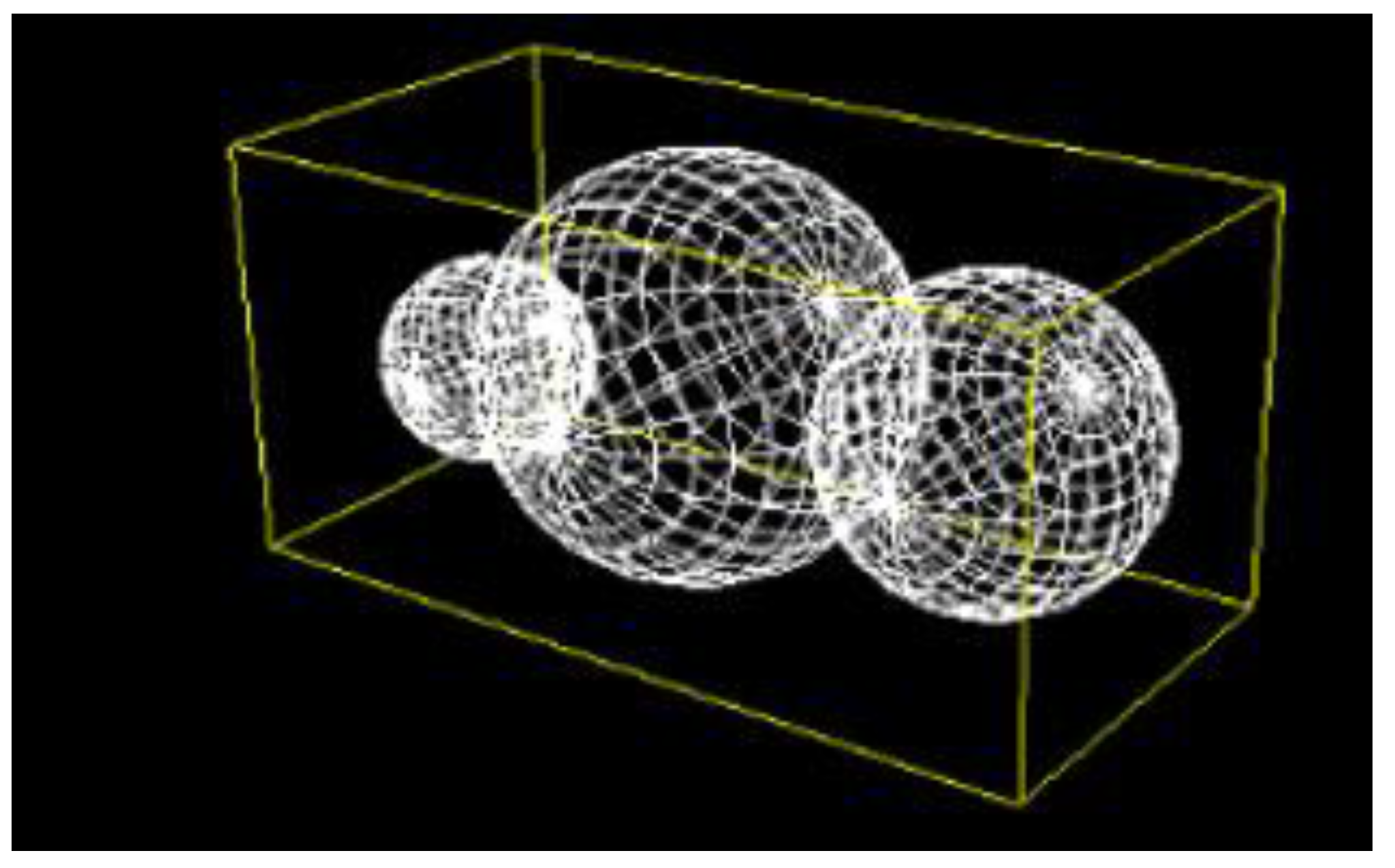
2.3. Solving the Bounding Box

Assume that the center coordinates of the three balls are $\left(x_1,y_1,z_1\right)$, $\left(x_2,y_2,z_2\right)$, and $\left(x_3,y_3,z_3\right)$ respectively, their radii are R₁, R₂, and R₃, respectively. The first thing is to calculate the rectangular bounding box. Assume that the coordinates of the minimum vertex of the bounding box are $\left(x_{\text{min}},y_{\text{min}},z_{\text{min}}\right)$, and the coordinates of the maximum vertex are $\left(x_{\text{max}},y_{\text{max}},z_{\text{max}}\right)$, then:

$$\{\begin{array}{l}{x}_{\min }=\min \{x_1-R_1,x_2-R_2,x_3-R_3\}\\ y_{\min }=\min \{y_1-R_1,y_2-R_2,y_3-R_3\}\\ z_{\min }=\min \{z_1-R_1,z_2-R_2,z_3-R_3\}\end{array}$$

(1)

$$\{\begin{array}{l}{x}_{\max }=\max \{x_1+R_1,x_2+R_2,x_3+R_3\}\\ y_{\max }=\max \{y_1+R_1,y_2+R_2,y_3+R_3\}\\ z_{\max }=\max \{z_1+R_1,z_2+R_2,z_3+R_3\}\end{array}$$

(2)

The circumscribed sphere of the three-dimensional contour can be obtained based on these two points. Assume that the center of the circumscribed circle is (x,y,z), that is (($x_{\text{max}}-x_{\text{min}})/2,$ $\left(y_{\text{max}}-y_{\text{min}}\right)/2,\left(z_{\text{max}}-z_{\text{min}}\right)/2)$, then the radius of the sphere based on geometric principles is $\mathrm{R} = \sqrt{{\left(x_{\text{max}}-x_{\text{min}}\right)}^2+{(y_{\text{max}}-y_{\text{min}})}^2+{\left(z_{\text{max}}-z_{\text{min}}\right)}^2}$. The inscribed rectangular of this sphere is the bounding box which generates cloud particles, as shown in Figure 3 and Figure 4. The three-dimensional shape of the cloud is the space which is composed of the three spheres.

We use two vertices along a diagonal line of the bounding box to describe the bounding box. The vertex whose coordinates are positive and the vertex whose coordinates are negative are used in this paper. The structure of the bounding box is as follows:

Struct BoundingBox

{Vector Origin;

Vector MinPt;

Vector MaxPt;

Line Boundaries [10];};

In the structure shown above, the “origin” represents the center coordinates of the bounding box, “MaxPt” represents the positive vertex, and “MinPt” represents the negative vertex. We can determine the size of the bounding box through the sphere radius and center coordinates of the circumscribed sphere. We use the center coordinates of three initial spheres to subtract the radius of the circumscribed sphere and compare the results. The minimum value is the MinPt. Similarly, add the center coordinates of each sphere to the radius of the circumscribed sphere, then the maximum value is the MaxPt. In order to facilitate post-drawing of the bounding box, the structure should contain a Line structure which represents the side information of the bounding box. The Line structure is defined as follows:

Struct Line

{Vector Origin;

  Vector End;};

Obviously, the “origin” in the Line structure indicates the starting point of a side of the bounding box, while the “end” indicates the ending point of the side. Figure 3 and Figure 4 show the effect pictures of the bounding box.

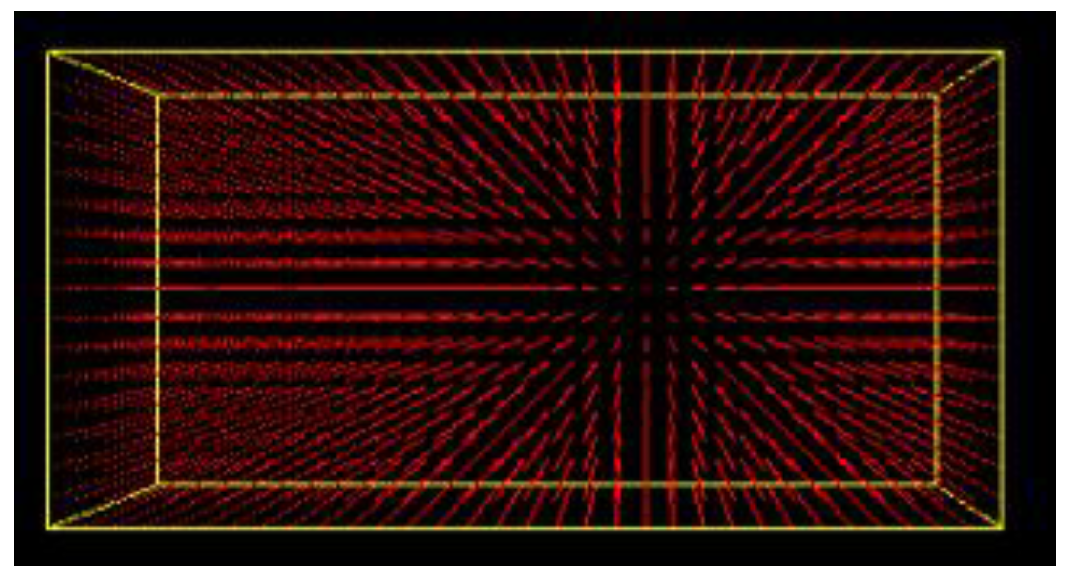
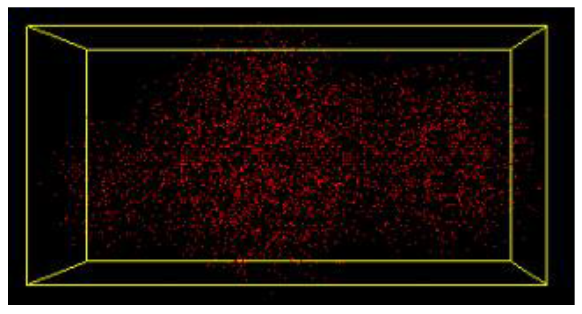
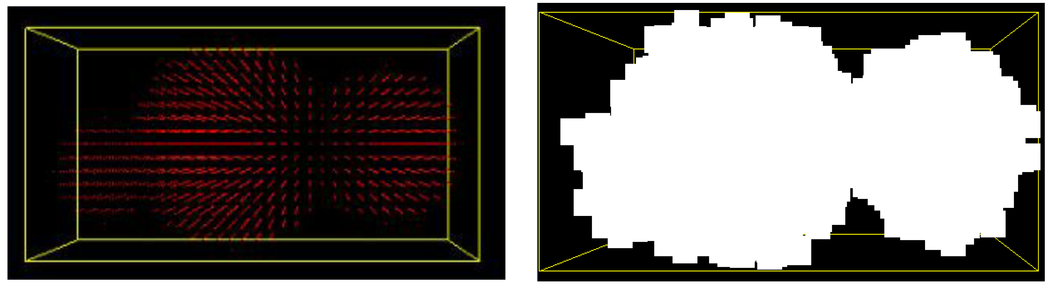
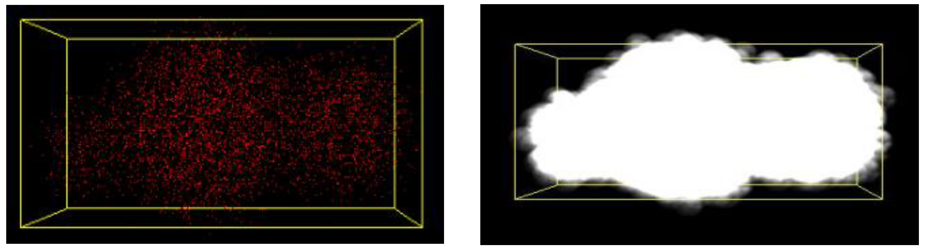
2.4. Generation of Particles in the Bounding Box

The particle system helps generate cloud particles in the bounding box. To produce cloud particles, two aspects should be taken into account. The first is the initial number of particles, followed by the size of the particles.

In the particle system, the generation of new particles is controlled by a random function. The random function randomly generates a certain number of particles within the given particle space, where the number of particles is the number of particles generated in one frame. This number determines the density of the cloud. If the number of particles is too small, then the lifelikeness requirements cannot be met. If it is too large, the data processing time will be increased, failing to meet the real-time requirements [10]. In order to satisfy both lifelikeness and real-time requirements, we use the following random function to determine the number of cloud particles.

$$N_{sum}=N_{frame}+rand()\times N_{\max }$$

(3)

where N_sum is the total number of particles generated in each frame, N_frame is the number of particles in the rendering process of each frame, and N_max is the maximum change of the particle number.

Particle size has a significant impact on the fineness of clouds. According to human visual principles, when the viewpoint is far from the cloud center, human eyes are insensitive to the cloud, so we can use large-size particles. Conversely, if the viewpoint is near to the cloud center, human eyes are sensitive to the cloud and the fineness requirements are high, so we should reduce the particle size for rendering. This method ensures the lifelikeness of clouds and reduces the number of needed particles, improving the rendering speed. Figure 5 shows the drawing effect.

Then we use the three spheres to cut the uniform particles in the bounding box (shown in Figure 6), and delete the left particles and sphere parts. Figure 7 shows the results.

3. Simulating Cloud Particles Using the Cellular Automaton

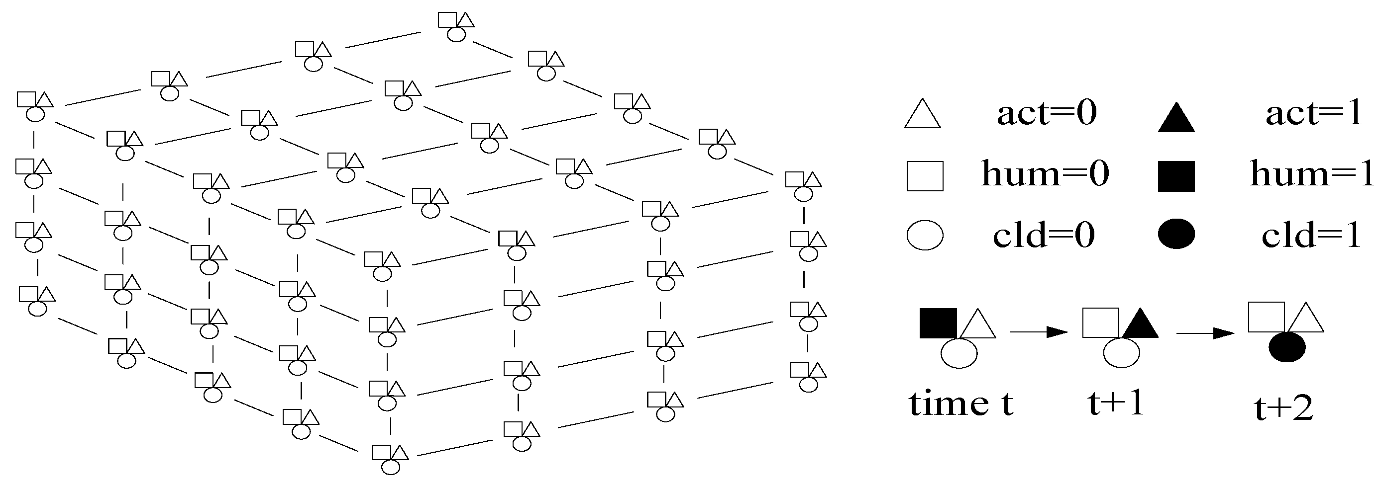
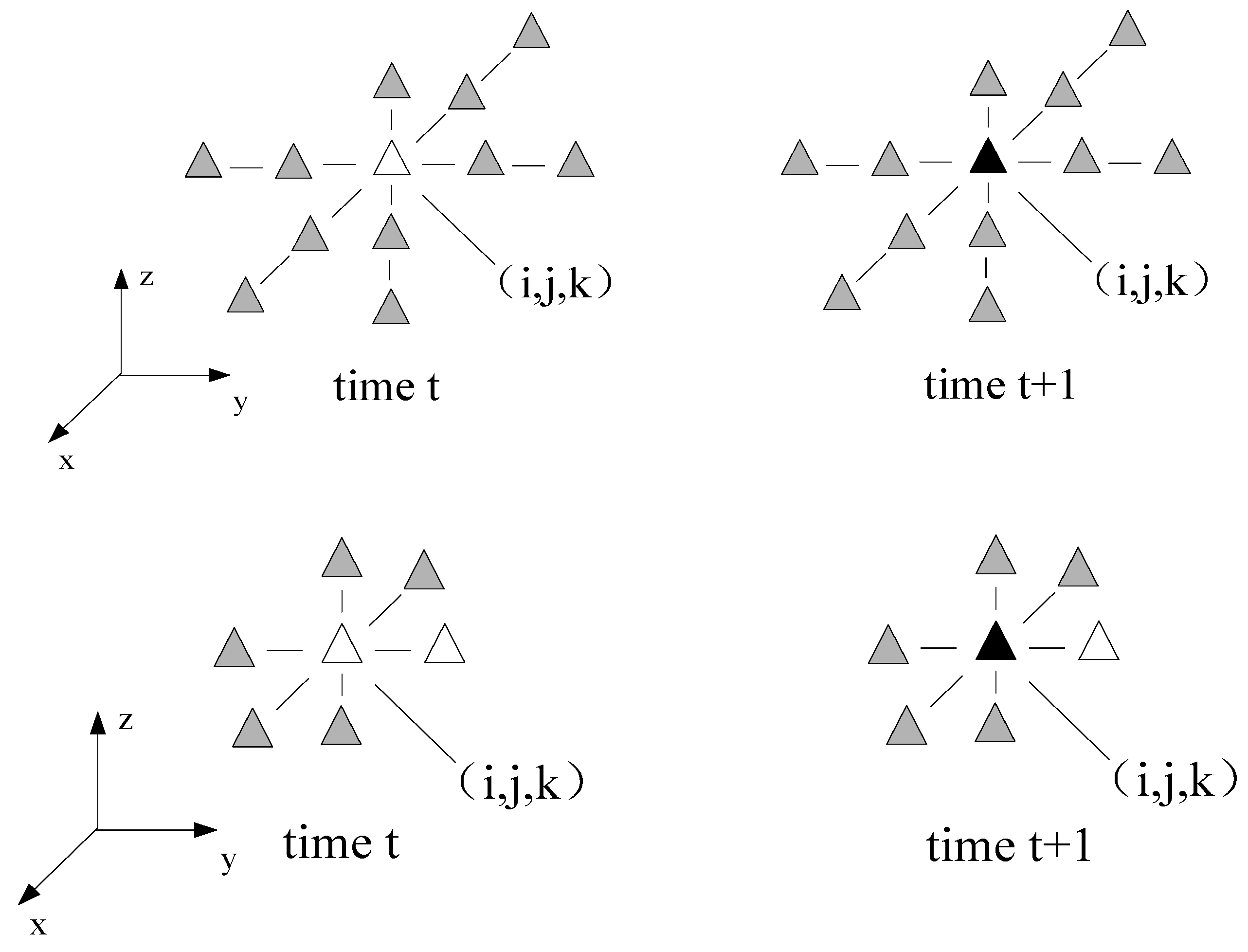
3.1. Overview of the Cellular Automaton

A cellular automaton is an idealized physical model which is discrete in space and time. Its physical parameters only have limited sets of values. According to the cellular automaton theory, the simulation space can be divided using 3D grids, as shown in Figure 8. Each grid represents a cell and each cell represents a vapor particles. All cells are given three state variables: hum, cld, and act, which represent water vapor, the cloud, and the changing state from water vapor to cloud (water) respectively. Each state variable has a value of 1 or 0. 1 indicates that vapor particles exist in the form of water vapor. 0 indicates that vapor particles exist in the form of ice crystals or cooled water droplets.

3.2. Using Cells to Replace the Uniform Particles

hum = 1 indicates that there is enough water vapor to form a cloud. act = 1 indicates the state change from water vapor to the cloud (water) is taking place. cld = 1 indicates that the cloud has been generated. Cloud generating is simulated using Boolean operations. Figure 9 shows the basic rules of cell state transitions. Assume that the states of a cell from t_i to t_i+1 change as follows: act changes from 0 to 1, hum changes from 1 to 0, and cld changes from 0 to 1, then the corresponding conversion formulas are:

$$hum(i,j,k,t_{i+1})=hum(i,j,k,t_i)\wedge \neg act(i,j,k,t_i)$$

(4)

$$cld(i,j,k,t_{i+1})=cld(i,j,k,t_i)\vee act(i,j,k,t_i)$$

(5)

$$act(i,j,k,t_{i+1})=\neg act(i,j,k,t_i)\wedge hum(i,j,k,t_i)\wedge f_{act}(i,j,k)$$

(6)

where f_act(i,j,k) is a Boolean operation function. Taking into account that tiny water droplets will rise and diffuse to the horizontal direction with the atmospheric motion, the value of this function should be determined by the act and hum states of 11 rounding cells. Thus, the function can be expressed as:

$$\begin{array}{l}{f}_{act}(i,j,k)=act(i+1,j,k,t_i)\vee act(i,j+1,k,t_i)\\ \vee act(i,j,k+1,t_i)\vee act(i-1,j,k,t_i)\vee act(i,j-1,k,t_i)\\ \vee act(i,j,k-1,t_i)\vee act(i-2,j,k,t_i)\vee act(i,j-2,k,t_i)\\ \vee act(i+2,j,k,t_i)\vee act(i,j+2,k,t_i)\vee act(i,j,k-2,t_i)\end{array}$$

(7)

We can use Equations (4) to (7) to control the cloud generation. However, we find that the cld will always maintain 1 after it changes to 1. Therefore, a new state variable is introduced to solve this problem. At first, we define a vanishing probability pext and then generate a random value rnd (ranging from 0 to 1) for all cells whose cld is 1. If rnd < pext, then the cld becomes 0. Similarly, the corresponding vanishing probability phum and pact of the hum and act are also defined, respectively. If rnd < phum, then hum = 1. If rnd < pact, then act = 1. The formula is described as follows:

$$cld(i,j,k,t_{i+1})=cld(i,j,k,t_i)\wedge IS(rnd>pext(i,j,k,t_i))$$

(8)

$$hum(i,j,k,t_{i+1})=hum(i,j,k,t_i)\vee IS(rnd<phum(i,j,k,t_i))$$

(9)

$$act(i,j,k,t_{i+1})=act(j,i,k,t_i)\vee IS(rnd<pact(i,j,k,t_i))$$

(10)

With above seven formulas, we can control the state values of each cell, obtaining the discrete density model of the cloud.

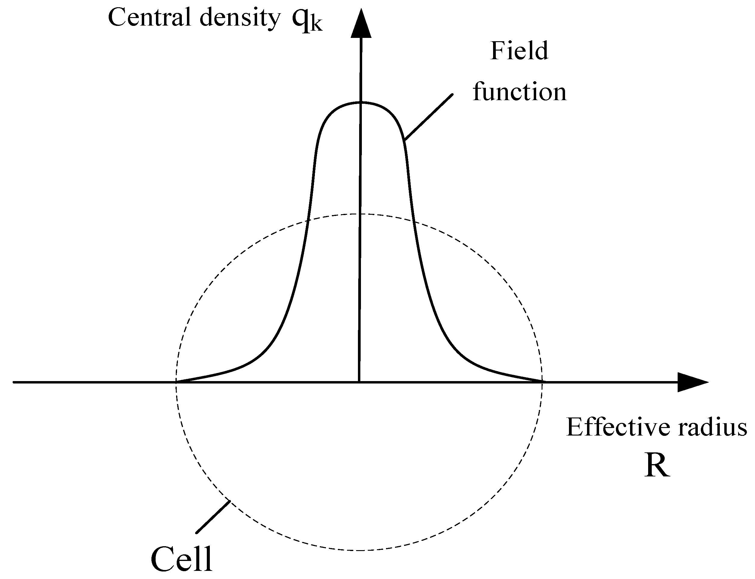
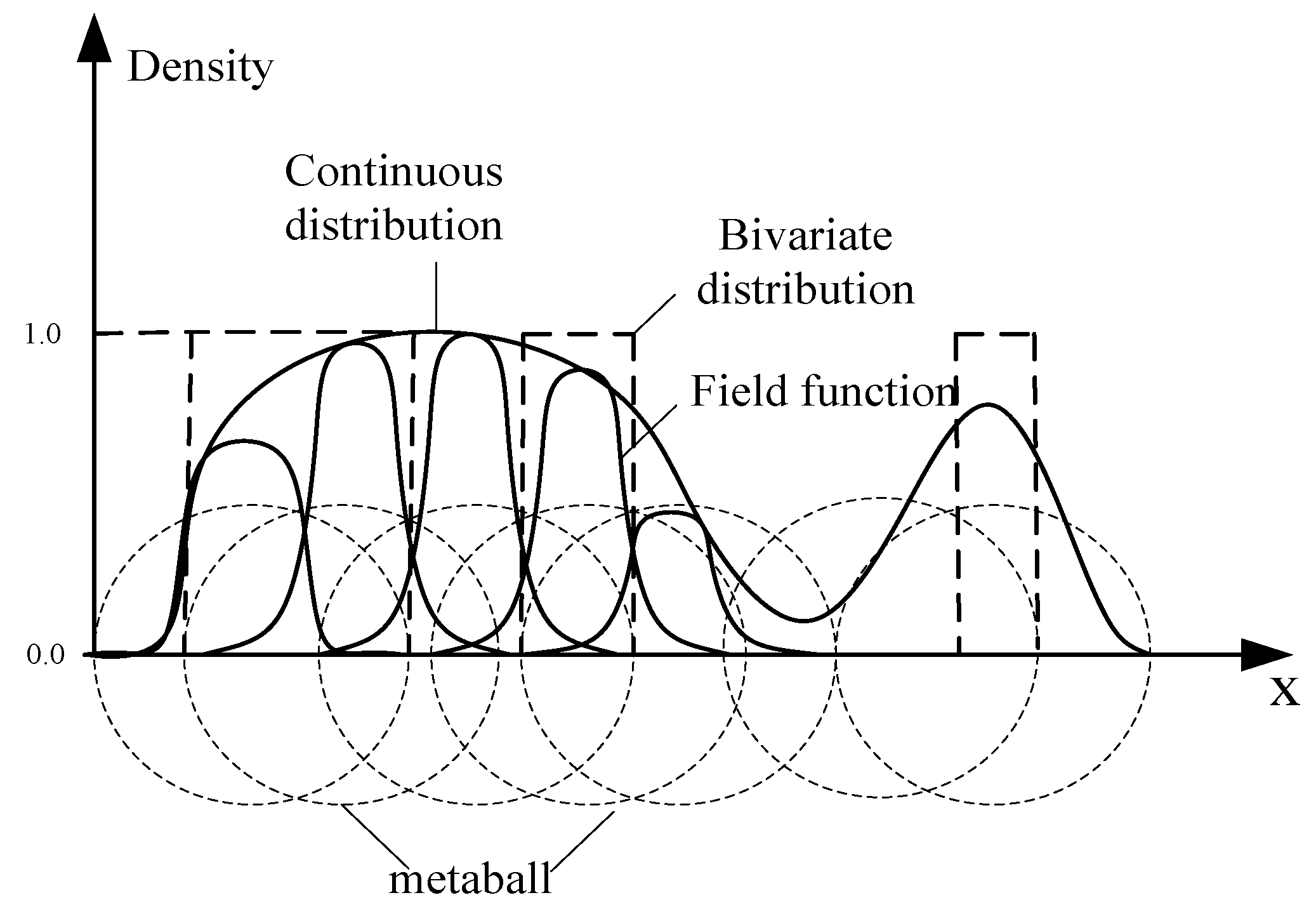
3.3. Calculating Continuous Density

A cell has two parameters: The central density and the effective radius. As shown in Figure 10, the vertical axis represents the density and the horizontal axis represents the distance from the center to the cell. Each cell is a sphere defined by a field function. We use the cellular automaton to calculate the continuous density distribution. For simplicity, we define a dimension to represent the continuous density distribution. As shown in Figure 11, the cells are placed on grid points, then the weighted sum of field functions represents the continuous density distribution. Continuous density distribution can be obtained by adjusting the center density and effective radius based on the binary distribution. The effective radius R can be assigned.

$$f(r)=\{\begin{array}{ll}-\frac{4}{9}{a}^6+\frac{17}{9}{a}^4-\frac{22}{9}{a}^2+1& (r\le R)\\ 0& (\mathrm{r}>R)\end{array}$$

(11)

We assume that cld is the discrete density value. X_l,m,n represents the coordinates of the cell (l,m,n). Ω(X_l,m,n) is the cell set whose cells satisfy |X_i,j,k − X_l,m,n| < R in the metaball. N is the number of cells in the metaball. Then the cell density q at the metaball center can be obtained using (12):

$$q_{\mathrm{i},\mathrm{j},\mathrm{k}}=\frac{1}{n_c}\times {\displaystyle \sum _{l,m,n\in \Omega ({{\rm X}}_{l,m,n})}^{n_c}cld({{\rm X}}_{l,m,n})}$$

(12)

The continuous density of the cloud at some point can be calculated after obtaining the density of the metaball. The continuous density of the cloud can be expressed as:

$$\rho （{\rm X}）={\displaystyle \sum _{i,j,k\in \Omega ({\rm X})}^{\mathrm{N}}{q}_{i,j,k}f(\left|{\rm X}-{{\rm X}}_{i,j,k}\right|)}$$

(13)

where Ω(X) is the set of all cells which are centered at X and have radii of R. The density of each point can be obtained by using the density of each metaball and the sum of products of its weights at this point. The weights of the metaball on this point can be obtained by calculating the Murakami function (a constant function).

The uniform cloud particles produced by the particle system are processed according to the rules of cellular automaton. As shown in Figure 12, the continuous particle density is calculated, obtaining the final simulated cloud particles.

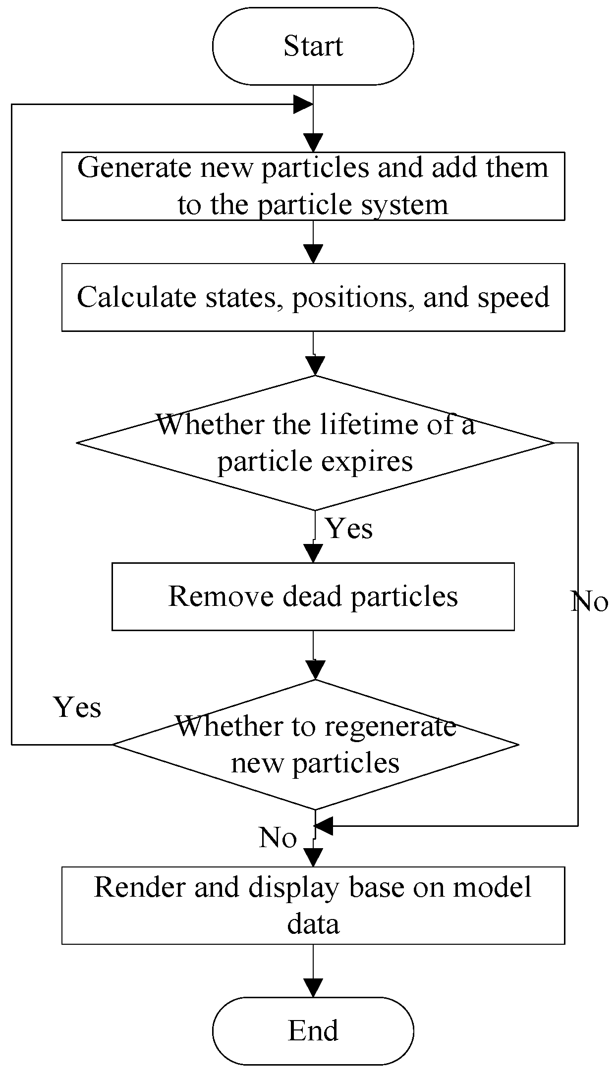
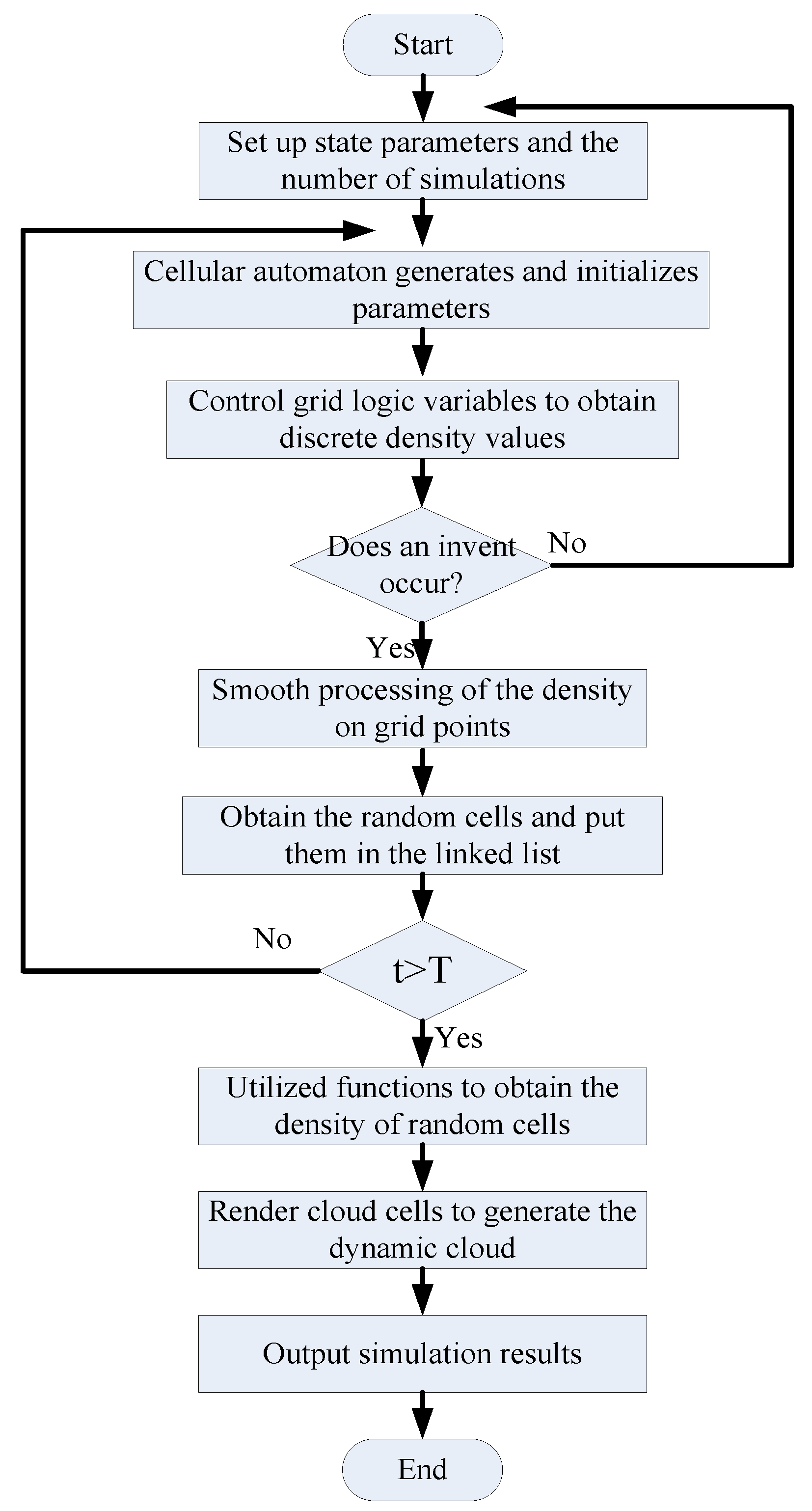
3.4. Flowchart of the Cellular Automaton Simulation

When using a cellular automaton model to simulate three-dimensional clouds, we need to initialize parameters first. Then based on the parameter status of each moment, we need to determine the parameters of the next moment according to certain rules. Figure 13 shows the specific flow chart of the cellular automaton simulation.

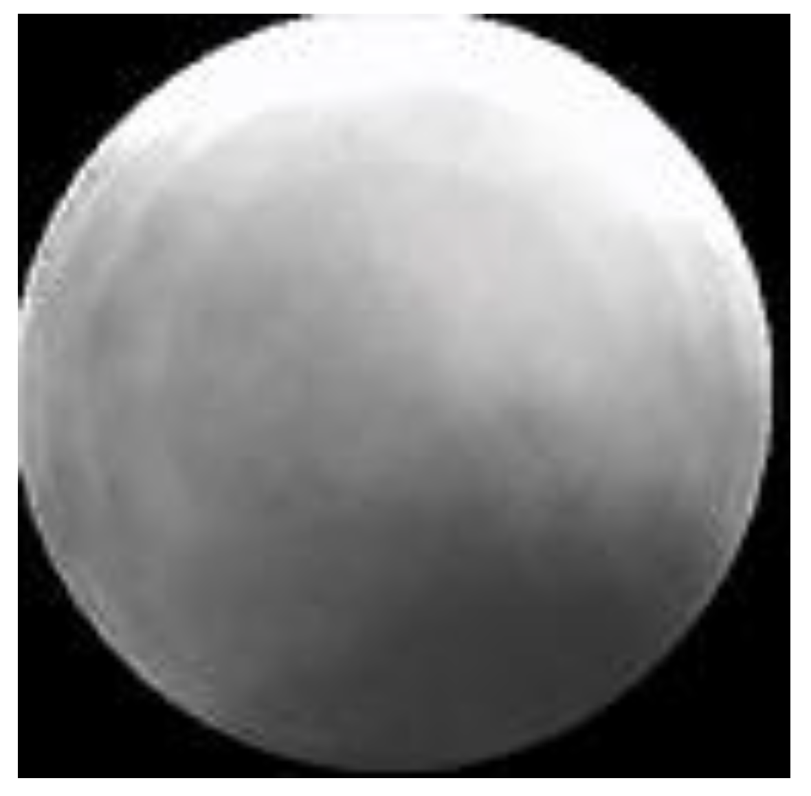
4. Texture Rendering

In the 3D visualization of the cloud, every cloud particle needs to be attached with a texture. The single texture in this paper is described in the RGBA form and R = G = B = A. A is the transparency. Transparency is inversely proportional to the grayscale value because the thickness of the cloud particles decreases from the center to the edge. The grayscale value of cloud particle texture should also be consistent with this rule. It also must have the capability of continuous transition. We can use Gaussian distribution to simulate this trend and the formula is [8,11,12]:

$$h(d)=\frac{\rho }{\sqrt{2\pi }\sigma }\exp (-\frac{d^2}{2{\sigma }^2})$$

(14)

where d represents the distance from the sphere center. h(d) represents the grayscale value of the texture at the d from the sphere center. σ is the variance of Gaussian distribution and we set it to 3. $\rho$ is the modulation value of the central peak. It should be 0.4 according to the simulation results and $\rho$ = σ in this case. Figure 14 shows the generated texture map.

The cloud particles generated in Figure 12 are added with the texture mapping in Figure 14. Figure 15 shows the final effect.

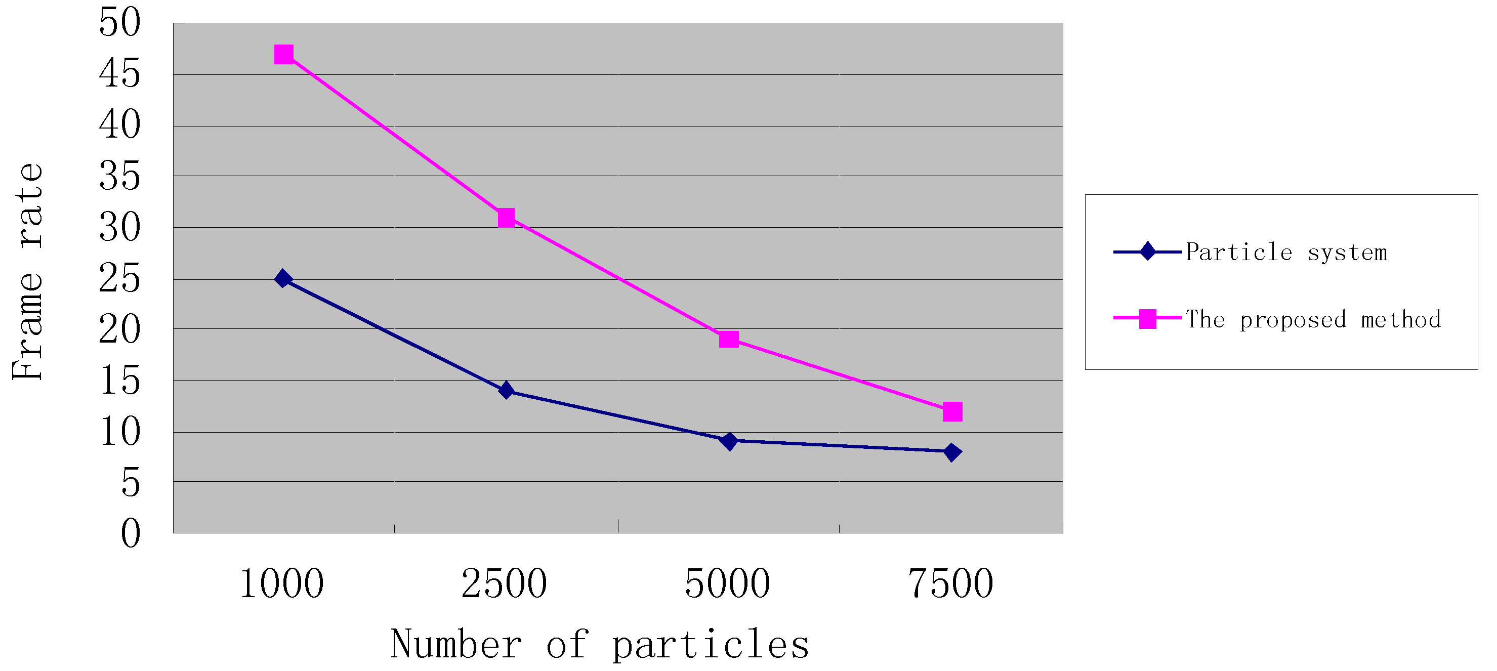
5. Results and Analysis

Harris et al. [13] used Impostor technology to accelerate the clouds using the correlation between frames in order to achieve real-time rendering of the scene requirements. However, in this kind of rendering method, the clouds size, position, and color are fixed. He Huaiqing et al. [14] improved Gardner ellipsoid model, and achieved good effect on penetrating the clouds, but this model has lack of liquidity and light simulation of the clouds. Lu Huaxing [15], Huang Bing et al. [16] used a modeling method based on particle systems, and have combined law motion and illumination model of clouds to obtain real results. Tang Zhao et al. [17] has solved the problems that occurred in using impostor technology application in alpha fusion scene and improved the clouds rendering speed. However, the above method does not solve the problem of large-scale realistic and smooth three-dimensional rendering of the clouds. Wang [18] used camera-oriented regular octagon rings to realize impostor technology, reducing the number of triangles drawn and accelerated the speed of rendering clouds. The advantage of this approach is that the formation of clouds is completed before rendering, and the rendering process does not need to calculate the shape of clouds, so the cloud rendering efficiency is very high and has also a strong sense of reality. However, the approach can not achieve a smooth light processing and self-shadowing effect. Li Gang et al. [19] proposed a framework totally based on the GPU to simulate and rending the three-dimensional clouds. In rendering the clouds, he used bitonic sort method implemented on the GPU to the composition of the three-dimensional clouds patch sorted for proper alpha blending. However, this method requires additional time overhead and hardware support. He Xiaoxi et al. [20] proposed an improved three-dimensional clouds simulation. In real-time rendering of the clouds, he proposed a lighting model based on the sunlight direction and the weather conditions, and used an improved cyclic mpostor technology to improve a wide range of clouds rendering speed.

The proposed method in this paper utilizes the particle system to simulate the user-defined cloud contour quickly and generates the initial cloud particles by taking advantage of the particle system. Then we use the cells in the cellular automaton to replace the initial particles and convert them according to the rules of cellular automaton. Finally, the related OpenGL technologies are used to render the cloud. Figure 16 and Figure 17 show the comparison between the combined methods proposed in this paper and the particle system algorithm.

According to experiments, the method proposed in this paper can implement the 3D simulation of clouds with very good lifelikeness. In addition, various cloud shapes can be obtained by changing the number of simulating spheres. The simulated cloud obtained using the combination of two methods in this section is more real than that obtained using only the particle system.

To better illustrate the advantages of the proposed method, we compare the performance of the proposed method and the particle systems. The experimental hardware includes: Pentium (R) Dual-Core 2.8 GHZ processor, 2.00 GB memory, and Windows XP (OS).

However, it can be seen from

Table 1. Comparison of results of different cloud modeling methods.

Algorithm Comparison	Particle System	Algorithm	Method in This Paper
Modeling method	Particle system	Cellular automaton system	Particle system + cellular automaton system
Whether it can customize the cloud contour	Yes	No	Yes
Lighting simulation	Impostor	Single reflection	Impostor
Three-dimensional cloud	Yes	Yes	Yes
Whether it contains movement	Yes	Yes	Yes
Whether it is a real-time algorithm	Yes	Yes	Yes

that the proposed algorithm and the traditional particle system algorithm are both real-time algorithms. In order to compare the real-time performance of these two methods, performance experiments are carried out. The most important performance of real-time algorithms is the number of rendered frames per second. The number of particles in the experiments is 1000, 2500, 5000, and 7500. Experiment results have shown that the performance of the proposed method in this paper (combining the particle system with the cellular automaton) is better than the traditional particle system. Figure 18 shows the frame rate comparison.

6. Conclusions

The basic concepts, principles, and workflow of the cellular automaton and particle system are described in this paper. First, we use a random function to generate uniform particles in the bounding box of a cloud, establishing a cloud particle system. We also initialize the related properties of particles, such as number, size, and location. Then we utilize the rules of cellular automaton to process the uniform particles simulated by the particle system and calculate its continuous field density, obtaining the final cloud particles. After that, texture mapping is used to render cloud particles, obtaining a lifelike three-dimensional cloud.

According to experiments, the method proposed in this paper can implement the 3D simulation of clouds with very good lifelikeness. In addition, various cloud shapes can be obtained by changing the number of simulating spheres. The simulated cloud obtained using the proposed method is more real than that obtained using only the particle system.

In order to compare the real-time performance of these two methods, performance experiments are carried out. The number of particles in the experiments is 1000, 2500, 5000, and 7500. Experiment results have shown that the performance of the proposed method in the paper is better than the traditional particle system.

This method not only obtains the real effect in the simulation, but also improves the rendering performance.

References

1. Wang, B.; Peng, J.L.; Kwak, Y.; Kuo, C. Efficient and realistic cumulus cloud simulation based on similarity approach. In Proceedings of the International Symposium on Visual Computing’07, Nevada, CA, USA, 26–28 November 2007; pp. 781–791.
2. Wang, B.; Peng, J.L.; Kuo, C.J. Cumulus cloud synthesis with similarity solution and particle/voxel modeling. In Proceedings of the International Symposium on Visual Computing’08, Las Vegas, NV, USA, 1–3 December 2008; pp. 65–74.
3. Dobashi, Y.; Nishita, T.; Yamashita, H. Using metaballs to modeling and animate clouds from satellite images. Vis. Comput. 1999, 15, 471–482. [Google Scholar] [CrossRef]
4. Dobashi, Y.; Yamamoto, T.; Nishita, T. A controllable method for animation of earth-scale clouds. In Proceedings of the CASA’06, Geneva, Switzerland, 5–7 July 2006; pp. 43–52.
5. Liao, H.S.; Ho, T.; Chuang, J.; Lin, C. Fast rendering of dynamic clouds. Comput. Gr. 2005, 29, 29–40. [Google Scholar] [CrossRef]
6. Xu, H.L. Simulation of 3D Cloud Based on Particle System. Master’s Thesis, Wuhan University of Technology, Wuhan, China, 2010. [Google Scholar]
7. Lopes, A.; Brodlie, K. Improving the robustness and accuracy of the marching cubes algorithm for isosurfacing. Vis. Comput. Gr. 2003, 9, 16–29. [Google Scholar] [CrossRef]
8. Nishita, T.; Dobashi, Y.; Nakamae, E. Display of clouds taking into account multiple anisotropic scattering and sky light. In Proceedings of the ACM Siggraph’96, New Orleans, LA, USA, 4–9 August 1996; pp. 379–386.
9. Bi, S.B.; Zeng, X.W.; Pan, Q.Y.; Shi, Y. 3D simulation and predigestion algorithms for clouds images based on particle system. J. Syst. Simul. 2014, 11, 2630–2636. (In Chinese) [Google Scholar]
10. Hu, X.Y.; Sun, B.; Ling, X.H. An improved cloud rendering method. In Proceeding of the International Conference on Image and Graphics, Xi’an, China, 1 June 2009; pp. 853–858.
11. You, Y.J.; Kang, F.J.; Tang, K. Research of sea battlefield distributed virtual environment based on fractal. J. Syst. Simul. 2009, 21, 7190–7194. (In Chinese) [Google Scholar]
12. Tuo, Y.F.; Wang, W.; Qiu, K.; Song, F.H.; Yu, F.F.; Wang, Y.; Wang, Y.S. Application of 3D simulation technology of AWX format infrared satellite cloud image based on OpenGL. J. Meteorol. Environ. 2011, 27, 25–31. (In Chinese) [Google Scholar]
13. Harrism, M.J.; Lastra, A. Real-time cloud rendering. Comput. Gr. Forum 2001, 20, 76–84. [Google Scholar] [CrossRef]
14. He, H.Q.; Liu, H.H.; Liu, J.X.; Yang, G.Q. Improved simulation method on 3D clouds. J. Syst. Simul. 2008, 20, 2620–2623. [Google Scholar]
15. Lu, H.X. Cloud modeling and rendering. Aircr. Des. 2009, 29, 64–68. [Google Scholar]
16. Huang, B.; Chen, J.; Wan, W.G. Cloud rendering in flight simulation and its implementation. J. Shanghai Univ. (Nat. Sci.) 2009, 15, 342–345. (In Chinese) [Google Scholar]
17. Tang, Z.; Wu, P.B. Real-Time modeling and rendering of 3D Cloud and its application in industrial simulations. J. Comput.-Aided Des. Comput. Gr. 2007, 19, 1051–1055. [Google Scholar]
18. Wang, N. Realistic and fast cloud rendering. J. Gr. Tools 2004, 9, 21–40. [Google Scholar] [CrossRef]
19. Li, G.; Li, H. All in GPU real-time 3D cloud simulation. J. Syst. Simul. 2009, 21, 7511–7514. [Google Scholar]
20. He, X.X.; Chen, L.T.; Zhu, Q.X. Simplified fluid method for fast simulation of large three-dimensional cloud scene. Appl. Res. Comput. 2012, 29, 2357–2359. [Google Scholar]
Figure 1. Flow chart of a particle system.
Ijgi 05 00086 g001
Figure 2. Cloud contour composed of different spheres.
Ijgi 05 00086 g002
Figure 3. Bounding box in the side view.
Ijgi 05 00086 g003
Figure 4. Bounding box in the front view.
Ijgi 05 00086 g004
Figure 5. Bounding box filled with particles.
Ijgi 05 00086 g005
Figure 6. Spheres filled with particles.
Ijgi 05 00086 g006
Figure 7. Spheres filled with uniform particles.
Ijgi 05 00086 g007
Figure 8. Space division and cell state variables.
Ijgi 05 00086 g008
Figure 9. Rules for cell state transitions.
Ijgi 05 00086 g009
Figure 10. Definition of a cell.
Ijgi 05 00086 g010
Figure 11. Continuous density distribution of the cells.
Ijgi 05 00086 g011
Figure 12. Final cloud particles.
Ijgi 05 00086 g012
Figure 13. Flow chart of the cellular automation simulation.
Ijgi 05 00086 g013
Figure 14. Texture map of the particle.
Ijgi 05 00086 g014
Figure 15. Cloud added with the texture (front view and side view).
Ijgi 05 00086 g015
Figure 16. The cloud simulated with the particle system before and after adding texture.
Ijgi 05 00086 g016
Figure 17. The cloud simulated with the proposed method before and after adding texture.
Ijgi 05 00086 g017
Figure 18. Frame rate comparison.
Ijgi 05 00086 g018