
Reducing Building Conflicts in Map Generalization with an Improved PSO Algorithm


1
School of Resources and Environmental Science, Wuhan University, Wuhan 430079, China
2
Wuhan Geomatics Institute, Wuhan 430079, China
3
School of Geosciences, Yangtze University, Wuhan 430079, China
*
Author to whom correspondence should be addressed.
ISPRS Int. J. Geo-Inf. 2017, 6(5), 127; https://0-doi-org.brum.beds.ac.uk/10.3390/ijgi6050127
Submission received: 9 December 2016
/
Revised: 23 April 2017
/
Accepted: 23 April 2017
/
Published: 26 April 2017
(This article belongs to the Special Issue Intelligent Spatial Decision Support)
Abstract
:In map generalization, road symbolization and map scale reduction may create spatial conflicts between roads and neighboring buildings. To resolve these conflicts, cartographers often displace the buildings. However, because such displacement sometimes produces secondary spatial conflicts, it is necessary to solve the spatial conflicts iteratively. In this paper, we apply the immune genetic algorithm (IGA) and improved particle swarm optimization (PSO) to building displacement to solve conflicts. The dual-inheritance framework from the cultural algorithm is adopted in the PSO algorithm to optimize the topologic structure of particles. We generate Pareto optimal displacement solutions using the niche Pareto competition mechanism. The results of experiments comparing IGA and the improved PSO show that the improved PSO outperforms IGA; the improved PSO results in fewer graphic conflicts and smaller movements that better satisfy the movement precision requirements.
1. Introduction
During map scale reduction, graphic conflicts can arise between buildings and road symbols. For example, when a map is generalized from 1:5000 to 1:25,000, the area of the map is narrowed. This reduces the space available for symbol representation, and road and building symbols may become too dense or overlap as a result. Cartographers use map generalization operators (e.g., aggregation, elimination, typification, and displacement) to preserve the ability for humans to recognize the symbols. A primary operator in resolving graphic conflicts is the displacement operator.
During the displacement process, because road symbols typically have a higher priority than building symbols [1], the overlapping building symbols are often moved. Cartographers move the symbols based on the following cartographic constraint conditions: the symbol should move as little as possible, and its geometrical characteristics should not change [2]. Every building has different possible movement vectors, and the different movement vectors and different building positions constitute different displacement candidate solutions. The purpose of an optimal displacement algorithm is to search for a candidate displacement solution with minimal or no conflict. Due to the size of the randomly generated candidate solutions set, performing an exhaustive search to find the optimal solution is not practical. Instead, intelligent search algorithms such as maximum gradient descent, simulated annealing, Tabu search, the genetic algorithm (GA), and the immune genetic algorithm (IGA) [3,4,5,6,7] have been used to solve the displacement problem.
The particle swarm optimization (PSO) algorithm was first introduced by Kennedy and Eberhart [8]. Similar to a flock of birds foraging in a valley, every individual bird (a particle) determines the best location for acquiring food. At the individual level, this is called the personal best (pbest) solution. However, overall, the entire flock finds the best location for food; this is called the global best (gbest) solution. By exchanging velocity and location information among the pbest solutions, gbest solution, and every individual bird’s solution, the best solution for acquiring food is obtained.
The building displacement solution can be represented as chromosomes in IGA or as particles in PSO. In IGA, selection, crossover, and mutation are three transpositional operations used to find the best chromosome in the search space. In PSO, the best solution is generated through ‘flying’. Each individual solution is treated as a non-volumetric particle in the D-dimensional search space, and flies at a certain speed in the searching space. Its velocity is adjusted by considering its own and its companions’ flight experiences.
We employ the same immune genetic algorithm (IGA) implementation used by Sun [7] for building displacement; however, the IGA displacement result contains too many conflicts. Consequently, we devised an improved PSO algorithm in which PSO is combined with the cultural algorithm computational framework. We calculate the initial movement vector using cartographic displacement rules, and adopt that as an initial flying velocity template for the particles, using the buildings’ original positions as the initial particles’ positions. This approach reduces the graphic conflicts. Moreover, the total distance that buildings must be moved is below that found by the IGA.
The remainder of this paper is organized as follows. Section 2 summarizes previous studies on the displacement problem. Section 3 describes the basic concepts underlying the improved PSO algorithm. Section 4 introduces the map graphic conflict detection method and discussed the details of the improved PSO algorithm applied to building displacement, the initial movement vector template calculations and the movement vector adjustment mechanism. Section 5 describes the experiments performed to compare IGA with the improved PSO displacement algorithm, compares the results by analyzing the reductions in conflicts and displacement distance, and demonstrates that the improved PSO algorithm performs better than the IGA. Section 6 concludes our study.
2. Related Works
A successful displacement algorithm should address two main issues: it should resolve multiple conflicts and avoid generating secondary conflicts. Displacement is an interactive process among the map symbols. Additionally, displacement is triggered by conflicts between map objects during the map scale reduction process. Displacement is a map generalization operator that is sensitive to context; some building movements inevitably affect neighboring buildings as well. This situation is called displacement propagation. Because modeling displacement is a complex process, the displacement of map objects is a spatial optimization problem. Previous studies that modeled the displacement process using function optimization were at somewhat of a disadvantage [7].
Some pseudo-mechanical models include the Springs, the Finite Element Method (FEM), and the Beams models. The Springs model proposed by Bobrich [9] may be the first displacement-solving method to propose an energy minimization concept. The Springs method compares the linear features of cartographic conflicts to different types of springs [9,10]. Using the mechanics of materials and finite element analysis, Højholt [11] modeled displacement as a continuous shift in the elastic deformation of a plate. In the FEM model, the map space is divided into discrete triangular elastic plates using Constrained Delaunay Triangulation (CDT), and the plates are assigned different rigidity and boundary conditions to simulate the cartographic constraints among different map symbols. However, the method simulates the displaced map symbol using triangular elastic panel deformation; when the displacement distance is large, a triangular graphic traversal arises, resulting in an abnormal result.
Borrowing from computer visual pattern recognition, Burghardt and Meier [12] proposed a linear feature displacement model based on the Snakes model. A Snake is an energy-minimizing spline whose movement is affected by both internal and external forces. The external force is a displacement driving force, while the internal force maintains the spline’s geometric shape. This method is very suitable for determining linear feature displacement but is not suitable for determining object displacement within an area.
The Beams model was proposed by Bader [13,14]. This model not only inherits the advantages of the Snakes model but also has a graphic constraint structure that is more consistent with map objects. A ductile truss is used to conserve building relationships. The ductile truss is an elastic bar-and-chain structure composed of an elastic bar and a hinge. Under these assumptions, a stress analysis model using the mechanics of materials is established that finds an optimal displacement solution using the energy minimization principle. To apply the Beams model to building displacement, Bader [13] demonstrated a mechanism that could maintain the building relationships. However, the internal energy required to maintain the spatial structure was too large; thus, Liu’s work [15] reported that some map symbol conflicts could not be solved.
The most classical mathematical analytical model for displacement is the least squares method proposed by Harrie [2], which transforms the map object displacement problem into one of finding an optimum solution under interior and exterior constraints. Harrie [2] stated that the process for solving conflicts is restricted to a rubber sheet transformation. Although it borrows some concepts from the Snake and FEM models, this solution is an adjustment theory in geodesy.
Some intelligent combination optimization methods have been used for the displacement problem [3,4,5,6,7]. Ware [4] adopted a trial map symbol configuration, in which the map symbols are assigned to trial positions, and the goal of the algorithm is to reduce conflicts, using the simulated annealing approach, and map symbol displacement solutions were searched heuristically within the solution search space. Wilson [6] discretized the candidate displacement solutions and mapped them to chromosomes, using the genetic algorithm to search for the best displacement solution. Ware [5] authored a similar paper that illustrated how the genetic algorithm (GA) could be applied to the map symbol displacement problem, emphasizing how the crossover and mutation operations changed the solutions. Fei [16] categorized building symbols into four types according to their adjacent relationships with roads, and moved them using four different methods. Sun [7] combined the building symbol classification idea with the GA to establish an immune genetic algorithm (IGA).
Some scholars have explored the displacement problem using geometric and morphologic methods; Mackaness [17] introduced an algorithm to determine displacement based on Dewdney’s “unhappiness” algorithm which optimizes people’s positions at social gatherings. Basaraner [18] used a Voronoi graph to determine building displacement. In this approach, an operational area for displacement is formed by the overlay of the Voronoi area and a building buffering area. Lonergan and Jones [19] designed a method that combined iterative improvement based on maximizing nearest neighbor distances and compared the displacement results with the simulated annealing approach. Li used dilation and erosion operators for line displacement [20] and Li and Yan [21] illustrated the group morphological characteristics of building symbols. Zhang [22] developed a method to recognize center and side pattern alignments. Ai [23] proposed the idea that a building’s displacement vector can be considered as a vector in a vector field, introduced a movement vector recession function to describe movement propagations, and incorporated the building pattern recognition results by following Zhang’s work.
All these displacement optimization algorithms move map symbols with minimum displacement precision costs (a single building symbol moves no more than 0.5 mm [7]) in exchange for a minimum number of conflicts and secondary conflicts, and they preserve topological relationships and spatial structure. However, in the results, the map symbols have no regular distribution pattern; there are no appropriate mathematics, physics or mechanical models that can describe the distribution pattern of the resulting map objects.
The success of using intelligent combination optimization methods for displacement rests upon their cost function, which is a measurement that evaluates the displacement quality. The cost function used in this essay is a weighted summation formula of the conflict reduction and the distance by which the map symbols moved.
3. Improved Particle Swarm Optimization Algorithm
3.1. Ordinary PSO
The PSO algorithm regards a candidate solution for a problem as a particle [8]. First, the algorithm randomly initializes a swarm of particles, which can be considered as many random solutions. Through information exchange among the personal best particles, the global best particle and all other particles, a final best solution is found. This approach can be applied to virtually any problem that can be expressed in terms of an evaluation function called a fitness function in this paper. The particles fly through the D-dimensional search space by updating the position of the i-th particle at iteration k as shown in Equations (1) and (2).
where denotes the i-th particle’s position in the n-th dimension at the k-th iteration, and denotes the i-th particles’ velocity in the n-th dimension at the k-th iteration. Here, represents the i-th particle’s best position in the n-th dimension, and represents the best position of the entire particle group in the n-th dimension. The parameters w, c1, and c2 are constants, and r1 and r2 are random numbers between 0 and 1. In Equation (1), the inertia weight w is used to control the effect of the previous ‘flying’ velocity on the current velocity; a larger inertia weight indicates that the search is more global, whereas a smaller inertia weight indicates a local search. In our study, the n-th dimension means the n-th building symbol.
3.2. Cultural Algorithm and PSO
The PSO algorithm generates the final solution as the particle population evolves; PSO is a simulation of a biotic community behavioral pattern. A more precise description for the group evolution process can be found in the Cultural Algorithm.
The Cultural Algorithm (CA) was proposed by Reynolds [24] and is designed to incorporate the concept of human social culture and simulate human social-evolutionary processes. In human society, culture is considered a carrier that preserves information obtained by all the individuals in a society and is used to guide their behavior. Cultural inheritance provides information and guidance to new individuals of a society to help them adapt to their environment. Cultural inheritance is achieved at both micro and macro levels and consists of two spaces: the population space and the belief space. Micro-level evolution occurs in the population space, while macro-level evolution occurs in the belief space. At the micro-level, individual solutions are calculated in the evolving community and develop into knowledge information. At the macro-level, the knowledge group preserves prior knowledge information, and through exchange with the micro-level, guides the subsequent evolution at the micro-level, preserves acceptable knowledge, and abandons unacceptable knowledge.
Compared to the cultural inheritance framework of the CA, in the PSO algorithm, the belief space information is contained in the global best particle, the individual in the population space is a single particle, and the guidance of the belief space to the population space is achieved using a velocity evolution equation, as shown in Equations (1) and (2). Therefore, ordinary PSO is a simplified form of the CA.
The improved PSO algorithm adopted for building displacement in this paper is integrated with the CA computational frame proposed in previous works [25,26]. The topologic structure of particles means the pattern in which the particles are connected, and the topologic structure of particles in the PSO algorithm can be improved by the dual inheritance framework in CA; moreover, the dual inheritance framework in CA enhances displacement information exchange and sharing among the particles in the PSO. In the belief space, we adopt the crossover operation and a niche competition strategy to ensure that the best solutions are equally distributed on the Pareto front. A Pareto solution pool is used to maintain the optimality of the current Pareto solution. Following these alterations, the improved PSO algorithm can overcome the poor global searching ability of the PSO algorithm, which can easily become trapped in local optima.
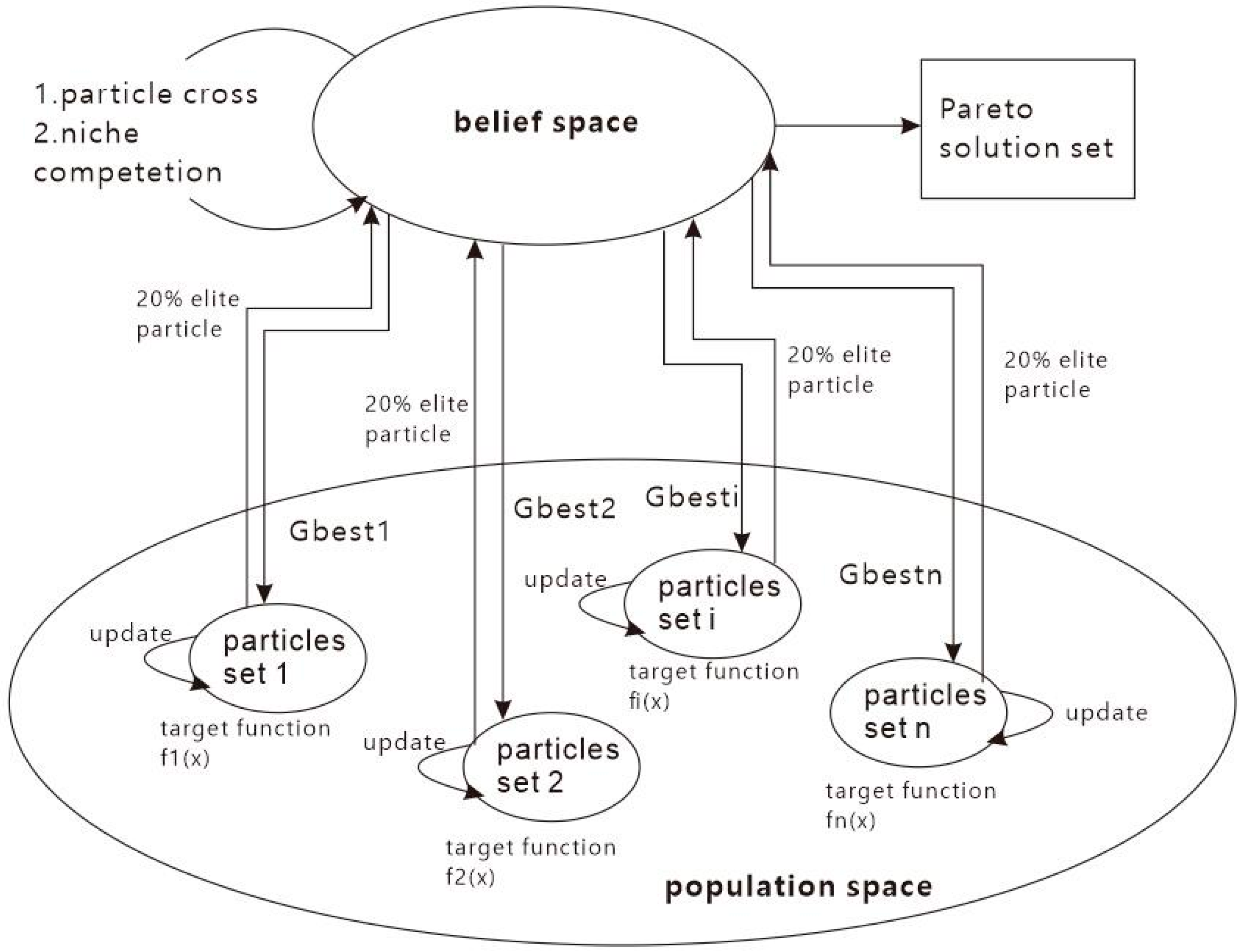
If there are n sub-populations in the population space as shown in Figure 1 and every i-th sub-population is assigned a fitness si(x) (i = 1, 2, …, q) function as its optimal objective function, then there are n optimal objective functions corresponding to n sub-populations. At the end of k-iterations, each sub-population group provides 20% of its elite particles to the belief space. These elite particles from different sub-populations constitute the belief space, and they adopt the crossover operation and niche competition to generate the Pareto optimal solution.
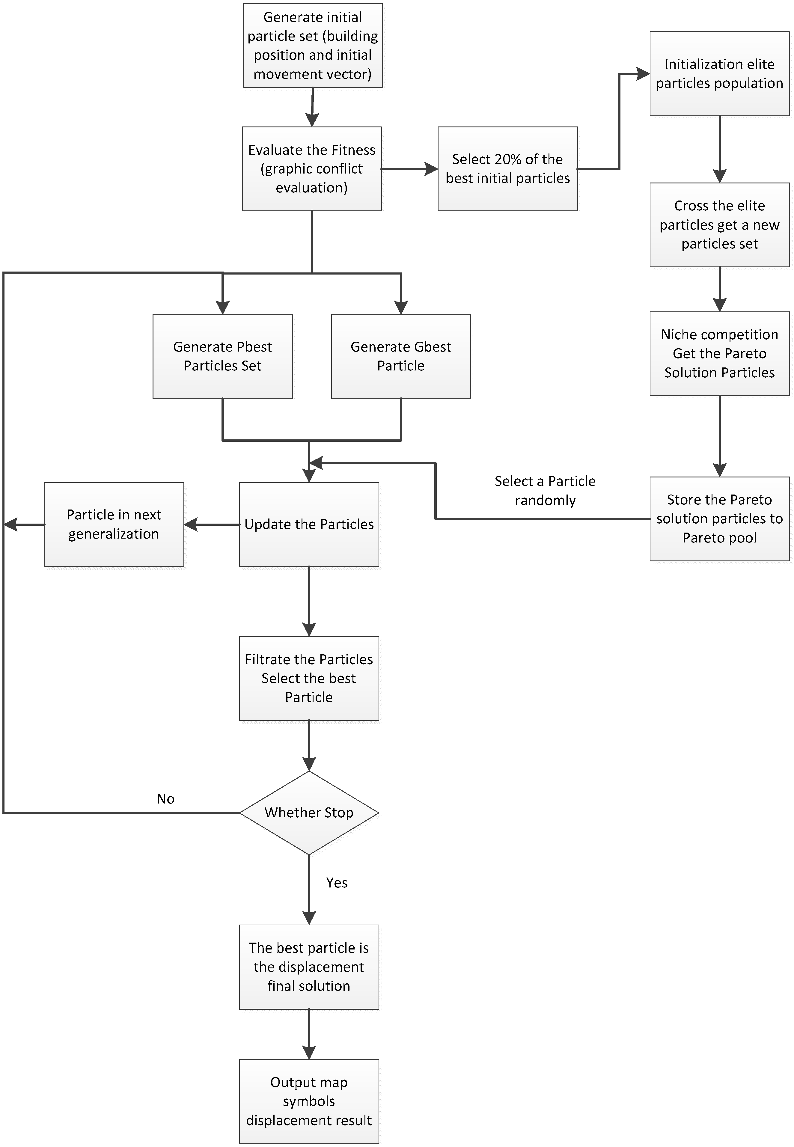
This improved PSO algorithm retains much similarity to the ordinary PSO algorithm. As described in Figure 2, the algorithm operates as follows:
- (1)
- Initialize the set of initial particles, calculate the fitness, and rank the particles according to their fitness values.
- (2)
- Select the top 20% of the elite particles that have the smallest fitness values from Step 1.
- (3)
- Generate the personal best (pbest) particle for each initial particle, and generate the gbest particle from the pbest sets.
- (4)
- Perform a crossover operation using the elite particles set from Step 2 to obtain a crossed particles set, conduct the niche competition for this set, obtain a Pareto solution particle, and store it in the Pareto solution pool.
- (5)
- Generate the next generation of particles.
- (6)
- Determine whether the terminal condition is met. When it is, stop the iteration and output the displacement result. When it is not, return to step 2.
3.3. The Pareto Optimal Solution
Because of the independence and complexity involved in comparing different candidate solutions, one solution may be best for some characteristics but poor for others. In the displacement problem, this means that a solution may solve some or all graphic conflicts in some parts of the map, but not in other parts. Hwang and Masud [27] illustrated the notion of a non-dominated solution or Pareto solution for optimality problems. A non-dominated solution is one in which no one objective function can be improved without simultaneously degrading to at least one of the other objectives. In the building symbol displacement problem, this means that one displacement solution cannot be improved without introducing new conflicts.
The Pareto solution (i.e., the non-dominated solution) is defined as follows. Assume any two solutions S1 and S2 in the solution set in which S1 is superior to S2 for all N targets; then, S1 dominates S2. When S1 is not dominated by the other solutions, S1 is called the non-dominated solution, i.e., the Pareto solution. Equation (3) shows a comparison of S1 and S2, where fk() represents the solution’s performance comparison function on target k.
The set of these non-dominated solutions is called a Pareto front. All solutions in the Pareto front are non-dominated by solutions outside the Pareto front.
Equation (3) can be explained in the evolutionary displacement algorithm discussed in this essay as follows. The function f represents the evaluation of the displacement result. S1 and S2 are the two candidate displacement solutions being compared. The Pareto optimal solution for displacement means that the movement solution has reached an optimal state and the algorithm cannot improve the movement solution. For each building k, the S1 displacement solution effect is better than the S2 solution.
4. Improved PSO Algorithm and Its Application in Building Displacement
In our improved PSO algorithm adapted to the building displacement problem, one particle represents one solution for displacing building symbols. The final best particle is the final building symbol displacement result. The particle’s flying velocity is a n-dimensional vector, denoted as ; this is the movement vector. The i-th particle position at time k is ; which represents the collection of building positions. The index i from 1 to n represents the building symbol id number. The PSO algorithm has a simple structure and requires fewer parameters than the GA, and it converges quickly.
As described in Equation (3), fk represents the solution performance on every single building k. To briefly evaluate the different solution particles, we define the fitness function in Equation (4).
where parameter n1 represents the building and a building conflict number, n2 represents the building and a road conflict number, and d3 represents the displacement distance of the building symbols. The parameters w1, w2, and w3 are weights.
The i-th particle flies to its best position using the fitness value evaluation defined in Equation (4). The pbest (personal best) particle set contains all the particles’ personal best positions which have minimum fitness values, and the gbest (global best) particle is the particle with the minimum fitness value from the pbest set.
The different particles represent the various positions and movement vectors of different building symbols. These particles share displacement knowledge through the dual inheritance framework described in Section 3.2.
4.1. Conflict Detection and Initial Movement Vector Calculation
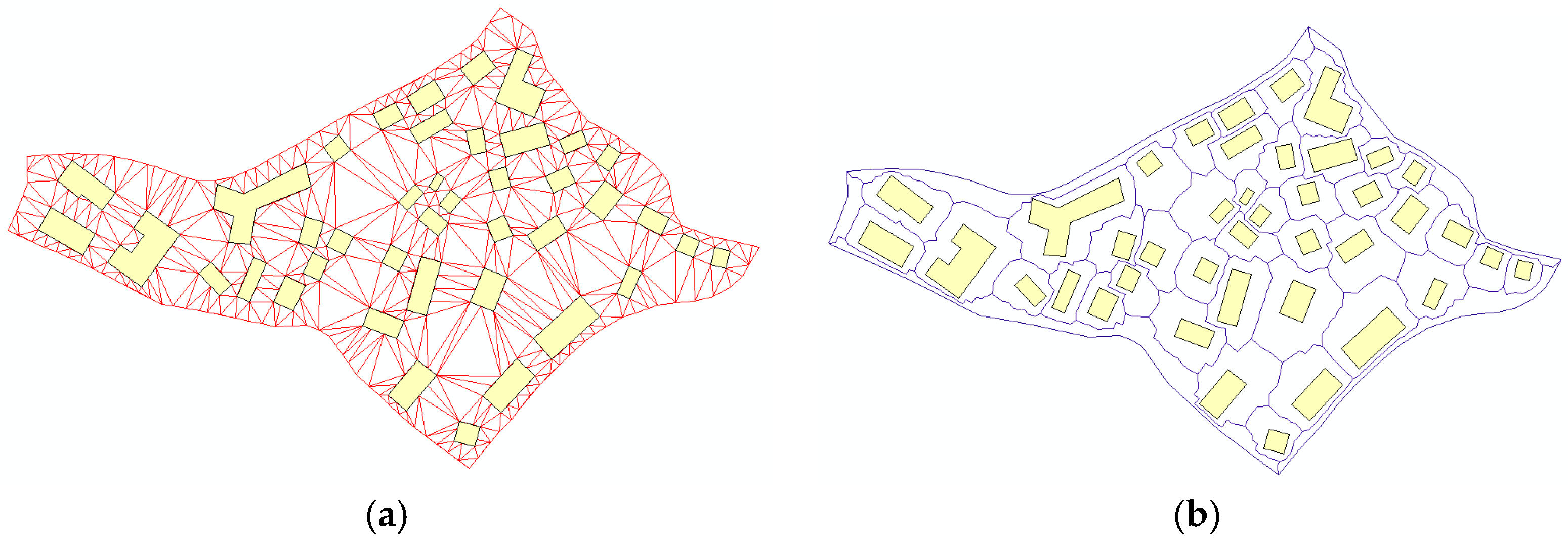
We generated a skeleton partition network based on CDT to explore the neighboring map symbol graphic conflicts (shown in Figure 3). The minimum distance threshold between two neighboring map symbols dmin is calculated using Equation (5).
where r1 is the rendering width of the map object symbol at the skeleton’s left, r2 is the rendering with of the map object symbol at the skeleton’s right, and dc is the minimum humanly recognizable resolution distance on the map and is set to 0.2 mm [6]. A conflict index is generated, which is convenient for conflict detection during the iterative movement process. The minimum distance between two map symbols is D. When D is less than the dmin threshold, a conflict occurs. The severity of the conflict sl is determined via Equation (6):
For clarity, Figure 3 does not show the width of the rendering symbol, but during graphic conflict detection, the rendering width of the symbol is calculated.
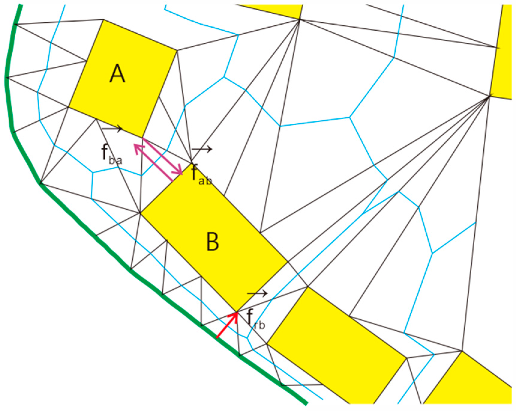
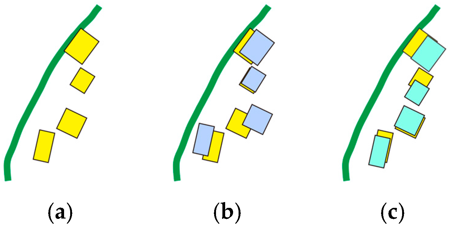
The combined initial movement vector template is calculated using the method in Liu et al. [15]. Two types of conflicts are distinguished: one is a conflict between a building and another building, called BB-conflict; the other is conflict between a building and a road, called BR-conflict. For BB-conflict, the area of two neighboring buildings is adopted as the weight for the movement vector calculation. For BR-conflict, the road segment is immovable; therefore, the movement vector template does not need to consider the area, as shown in Figure 4.
In Equations (7)–(9), AA and AB denote the areas of polygons A and B, respectively. and are weighted movement vectors, while and are the graphic movement vector directions between the two buildings in conflict (A and B). is the building B movement vector adjacent to the road, and is the graphic movement vector direction by the side of building B adjacent to the road.
Figure 5 depicts three graphic conflicts for building A: FB, FC, and FD. For the synthesis graphic vector calculation, we first assign the maximum graphic conflict vector FD as the main direction, establish the x-axis along it, assign the center of the conflict building as the origin point, and establish a local coordinate system. Then, we decompose all of the other conflict vectors (FB and FC) along the local coordinate system. Next, we find that the maximum decomposed conflict vectors in the positive direction and negative direction of the x-axis are FD and 0, while the maximum decomposed conflict vectors in the positive direction and negative direction of the y-axis are FBY and 0. The synthesizing vector on x-axis is ∑FX while on the y-axis it is ∑FY. Then we calculate the combined graphic conflict vector FC (shown as the green arrow in Figure 5d) with the ∑FX and ∑FY according to the parallelogram law from physics and mechanics.
In contrast to the work of Ware [4], we do not select a discrete random position as the candidate movement position; instead, we choose the combined graphic conflict vector as the initial possible movement template vector for the improved PSO algorithm. The movement template vector is shown in Figure 6. The green lines represent the roads.
4.2. Movement Vector Adjustment Mechanism
The initial movement template vector is defined in Equation (10), where F is the composition vector of the graphic conflicts that is calculated by the method described in Section 4.1 and is a random number between 0 and 1:
The initial displacement template vector set is vinit = {vinit_1, vinit_2, …, vinit_n}; this represents the velocity information in a displacement solution particle Pi, n is the number of buildings, and every velocity vector vinit_i (i = 1, 2, …, n) corresponds to information about a building’s movement.
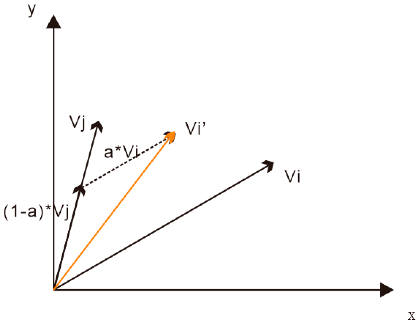
To enhance the polymorphism of the individual solutions’, we adopt the crossover operator applied to the elite particles. The crossover operation is defined in Equations (11) and (12). For every particle in the selected elite particle set, we cross the velocity of the two particles to generate two new velocities, which we assign to the two newly generated particles:
where vi is the velocity of particle Pi, vj is the velocity of particle Pj, and and are the two new velocities. This process resembles two vector combinations that cause the adjustment of the building movement vector. Therefore, the movement vector is modified in two ways in our work: one modification occurs during velocity updating as shown in Equations (1) and (2); the other occurs during the elite particles’ velocity crossover operation. If the velocities vi and vj have different directions, then the movement vector direction is modified as shown in Figure 7. The velocity vi’ is denoted by an orange arrow in Figure 7. After the crossover operation, the velocities vi and vj generate a new velocity vi’.
After performing the crossover operation, a selection mechanism based on the niche Pareto competition will be performed to pick the excellent particles for replication. These excellent particles are copied into the Pareto solution pool. The niche Pareto competition operates as follow:
Select any two particles from the crossed particles set. If one dominates the particle set and the other does not, copy the non-dominated particle to the Pareto solution pool. Domination is judged according to Equations (3) and (4).
When both particles dominate or are dominated by the particle set, the particle with the smaller niche number is selected and copied to the Pareto solution pool. The niche number mi is calculated by summing the sharing function within the whole population as shown in Equations (13)–(15).
In the preceding equations, mi is the niche number, SN is the particles’ swarm size, sh(·) is the sharing function that represents the similarity between two individual particles, a is set to two in our work, and σshare is the niche sharing radius. To reduce the computational time required, we calculate only the particles’ similarity within the niche sharing radius, dij is the normalized fitness value distance between particle i and particle j, fmin is the minimum fitness value, and fmax is the maximum fitness value. The elite particles are copied to the Pareto solution pool. As stated in Section 3.2, the belief space is composed of the elite particles, enabling the entire population to share the excellent displacement information contained in the elite particles. Consequently, after the crossover and selection operations are complete, the belief space should guide the evolution of the population space. This goal is achieved by adding a correction term to the particle velocity updating operation in Equation (1), as shown in Equation (16).
The , , , , w, c1, c2, r1, and r2 notations are defined in Section 3.1. The is a randomly selected Pareto optimal solution from the Pareto pool, and is the correction term added to Equation (1).
5. Comparative Experiments
5.1. Two Experiments
We applied the GA and the improved PSO displacement algorithm to the same region of Wuhan City in China. The region consists of 256 polygons and 7 closed roads. The buildings are separated into 7 blocks by the closed roads: these are partitions D1B, D2B, D3B, D4B, D5B, D6B and D7B. The original scale was 1:5000, which was reduced to a scale of 1:25,000. The road width is 0.2 mm. Due to the map scale reduction, there are initially 222 graphic conflicts, as shown in Figure 8a. We implemented the displacement procedure using Microsoft Visual Studio 2010 in the C# language, running on the ArcGIS engine on a PC with a Windows10 OS and Intel Core™ i5-4210M CPU.
The displacement procedure includes the initial movement vector calculation, the intermediate movement solution searching process, the displacement evaluation and outputs the displacement result.
We implemented the immune genetic displacement algorithm by Sun Yageng; the IGA theory is given in Sun’s work [7]. We defined the population size as 1280 following Sun’s work, the crossover rate as 0.8, and the mutation rate as 0.08.
We randomly generated 50 particles, each of which contained a randomly generated movement vector. Using the synthesis graphic conflict vector calculated by the method described in Section 4.1, we defined the initial movement vector as a random number between 0.2 and 0.5 multiplied by the movement template vector described in Section 4.1. According to Equation (1), the inertia weight w is used to determine how much of the particles’ previous velocity is preserved; a larger inertia weight indicates that the search is more global, while a smaller inertia weight indicates a local search: we set w to 0.9. For the particles’ “flying” operations (Equation (16)), c1 was set to 1.2, c2 to 2.3 and c3 to 1.2. Note that we set c2 larger than c1 to obtain a global search result; the settings used here are the same as those used in Gao et al.’s work [25]. At the end of each iteration, the top 20% of the elite particles from the particle set are selected, and the velocity crossover operation is performed according to Equations (11) and (12).
5.2. Analysis of Experimental Results
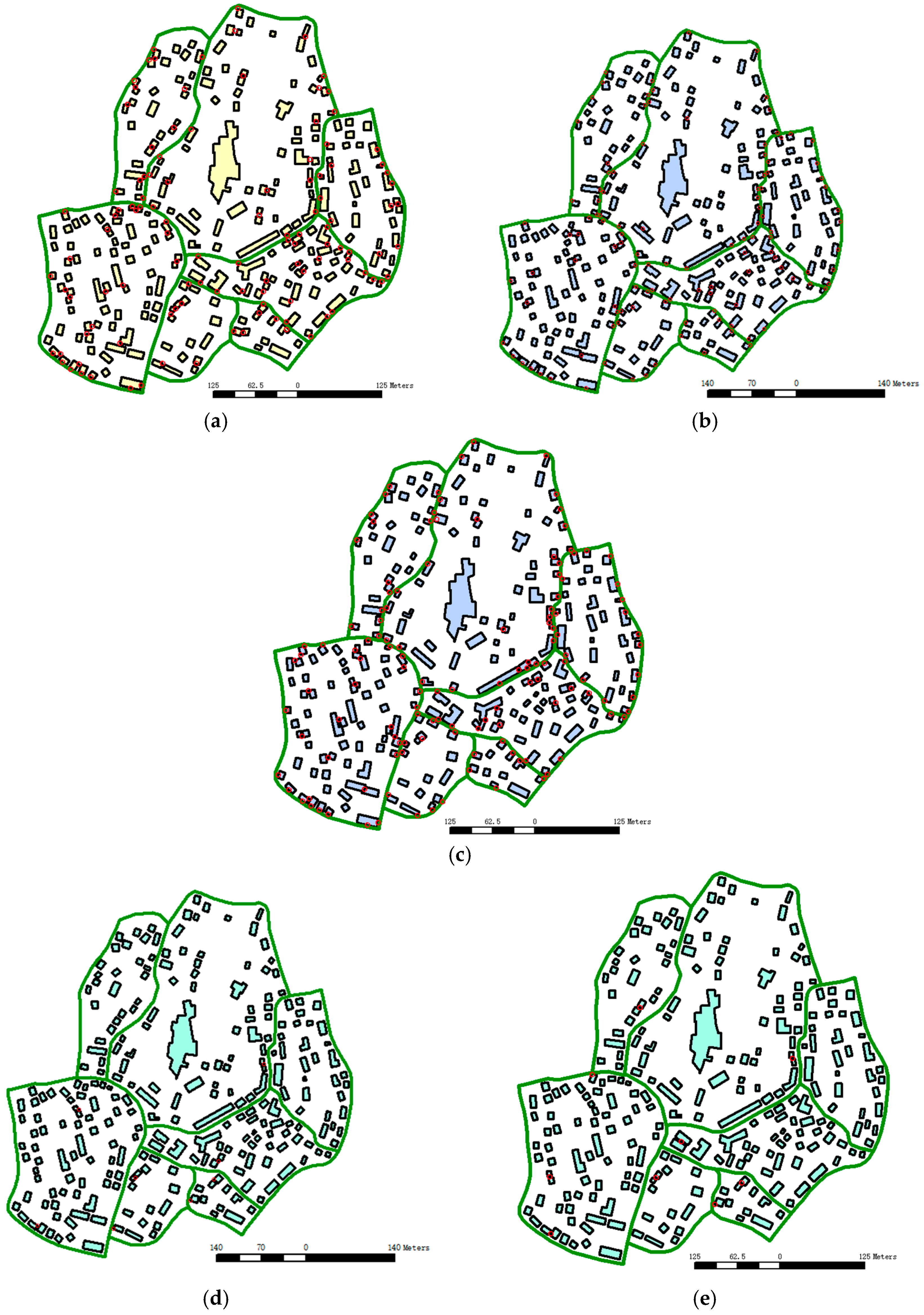
The displacement result evaluation considers two points. One is the reduction in total conflicts; the other is the total displacement distance. A shorter displacement distance represents a better displacement result. The original map, the displacement result map resulting from IGA, and the displacement result map resulting from the improved PSO are presented in Figure 8a–e.
We find that secondary conflicts occur in the IGA displacement result. Some concave polygons overlap with other polygons, and some polygons overlap at road corners. We suspect that the mutation operator applied to the movement vector in the IGA may cause buildings to overlap that initially had no graphic conflicts. The IGA algorithm has no memory and cannot preserve information concerning well-behaved displacement solutions. From Equations (2) and (16), we can deduce that the child solutions in the improved PSO have stronger connections with their parent solutions, because they inherit the movement information contained in the elite particles [26].
The building symbol displacement result is a slight adjustment that should satisfy the minimum legibility requirements (0.2 mm) [7]. In contrast, the genetic displacement result occurs with some secondary graphic conflicts; the improved PSO algorithm performs better.
As can be observed from the two displacement results shown in Figure 9, the IGA movement vector is longer and has a different movement direction than the improved PSO; through velocity information exchange, the movement vector of the improved PSO is shorter and represents a more reasonable direction. There are two reasons for this phenomenon: one is because the movement template vector initialization calculation method is different and the other is because the evolution mechanisms of PSO and IGA are different.
A comparison of the numerical indices of the displacement results from the IGA and the improved PSO algorithm are shown in Table 1, Table 2 and Table 3. The two algorithms were applied to the same map. Interestingly, we can see that the IGA produces secondary conflicts in some local regions; however, the improved PSO algorithm ameliorates this problem. In some crowded regions, the movement is often accompanied by movement vector propagation, which shows that displacement is a context-sensitive operation. This accompanying movement vector propagation refers to the process in which a building does not initially need be moved; however, the movement of adjacent buildings produces new conflicts. Subsequently, the building must be moved to reduce these new conflicts. The evaluation of a displacement result usually involves assessing whether secondary conflicts have been reduced.
After 10 iterations, IGA reduces the conflicts to 117, but nearly half of the initial conflicts remain unresolved. After 15 iterations, IGA reduces the conflicts to 95, but after 20 iterations, the conflicts have increased to 131, and the number of conflicts increases as the iteration number increases. There is a possible correlation between the IGA performance results and the number of iterations.
The improved PSO results solve the conflicts adequately. After 10 iterations, the conflicts have been reduced to eight and the conflicts remain almost the same after 15 and 20 iterations. The improved PSO algorithm solves the conflicts more successfully than does the IGA.
The improved PSO algorithm also performs well regarding the displacement distance. After 10 iterations, the IGA moves buildings a total of 232.21 m, whereas the improved PSO moves buildings by 34.79 m, only 15% of the displacement distance achieved by the IGA. After 15 iterations, the IGA displacement distance is reduced to 98.13 m, but the improved PSO displacement distance increased to 41.95 m, with only one conflict reduction. After 20 iterations, the IGA moved the buildings by 94.37 m, and the improved PSO moved the buildings by 42.02 m. This represents a slight increase in the displacement distance by the improved PSO without a corresponding improvement in conflict reduction.
As shown in Figure 10, the IGA performs abnormally with respect to the buildings in partition D3B. The displacement distance of the improved PSO after iterations 15 and 20 remains almost the same. The x-axis represents the partition number of the buildings, and the y-axis represents the displacement distance.
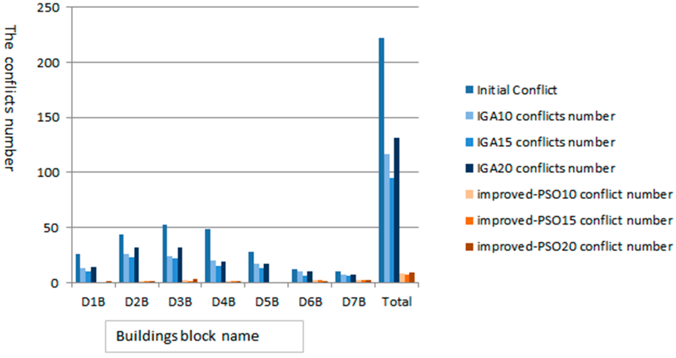
The IGA cannot effectively reduce the number of graphic conflicts, but the improved PSO algorithm can. From Figure 11, we know that after 20 iterations, the IGA displacement result includes more graphic conflicts than after 10 and 15 iterations. This result illustrates the IGA’s instability. The improved PSO results contain similar reductions in the number of conflicts and displacement distance after the three different numbers of iterations.
6. Summary
Our results indicate that the improved PSO displacement algorithm performs better than the IGA on the map data used in this experiment. The IGA displacement result with constrained movement directions resulted in more secondary conflicts than did the improved PSO algorithm. One reason for this result is that the improved PSO algorithm abandons the fitness function in IGA; instead, it adopts the fitness function in Equation (4) and does not calculate the displacement distance of buildings with the tangent relation constraint. Another reason is that the improved PSO’s mutation-like behavior is directional; the solution for the next generation takes advantage of the displacement knowledge from the elite solution of the previous generation. In IGA, the mutation operation is considered to be omnidirectional [28]; therefore, in the IGA result, the direction of building movements are significantly changed compared to the movement template vectors and, thus, cause the secondary conflicts.
The Pareto optimal solution is a global optimal solution that causes fewer secondary conflicts during the displacement process. The global displacement optimal solution considers every building movement situation. Through the movement vector adjustment mechanism, the symbols of every building move according to the displacement knowledge learned from the belief space.
The spatial structure cannot be precisely described by mechanical or mathematical analysis methods due to the irregular arrangement of the map symbols. We plan to address the map symbol secondary conflict-recurrence mechanism in our future work.
The improved PSO algorithm does not explicitly describe the spatial relationship maintenance schema because the fitness function is only a simple conflict number and displacement distance summation function. If the spatial structure and the relationship between the buildings were accurately described by the fitness function, the displacement results could be improved.
The graphic conflicts of buildings close to road corners is difficult to resolve. In narrow road corners, displacement problems are difficult to resolve because of the crowded building distribution. Therefore, we need to select fewer buildings for generalization. The experiments in this study involved low building densities, so that buildings would have sufficient space to move. When the change in map scale becomes large, buildings are necessarily arranged with high densities. Therefore, selection, deletion and aggregation operators for the buildings need to be considered, which is a different artificial intelligence decision problem beyond the scope of this paper.
Acknowledgments
This work was supported by the National Natural Science Foundation of China (Grant No. 41471384), and by the Scientific Research Program of Hubei Provincial department of education of China (Grant No. B2015448). The funders had no role in the study design, data collection and analysis, decision to publish, or preparation of this manuscript.
Author Contributions
Huang Hesheng designed and implemented the improved PSO algorithm for building displacement and wrote the paper. Guo Qingsheng reviewed the paper. Sun Yageng provided the source code for the IGA building displacement implementation. Liu Yuangang provided the source code for generating the constrained Delaunay triangulation.
Conflicts of Interest
The authors declare no conflict of interest.
References
- Ruas, A. A method for building displacement in automated map generalisation. Int. J. Geogr. Inf. Sci. 1998, 12, 789–803. [Google Scholar] [CrossRef]
- Harrie, L.E. The constraint method for solving spatial conflicts in cartographic generalization. Cartogr. Geogr. Inf. Sci. 1999, 26, 55–69. [Google Scholar] [CrossRef]
- Ware, J.M.; Jones, C.B. Conflict reduction in map generalization using iterative improvement. GeoInformatica 1998, 2, 383–407. [Google Scholar] [CrossRef]
- Ware, J.M.; Jones, C.B.; Thomas, N. Automated map generalization with multiple operators: A simulated annealing approach. Int. J. Geogr. Inf. Sci. 2003, 17, 743–769. [Google Scholar] [CrossRef]
- Ware, J.M.; Wilson, I.D.; Ware, J.A. A knowledge based genetic algorithm approach to automating cartographic generalisation. Knowl.-Based Syst. 2003, 16, 295–303. [Google Scholar] [CrossRef]
- Wilson, I.D.; Ware, J.M.; Ware, J.A. A genetic algorithm approach to cartographic map generalisation. Comput. Ind. 2003, 52, 291–304. [Google Scholar] [CrossRef]
- Sun, Y.; Guo, Q.; Liu, Y.; Ma, X.; Weng, J. An immune genetic algorithm to buildings displacement in cartographic generalization. Trans. GIS 2016, 20, 585–612. [Google Scholar] [CrossRef]
- Kennedy, J.; Eberhart, R.C. Particle swarm optimization. Proceeding of the IEEE International Conference on Neural Networks, Piscataway, NJ, USA, 27 November–1 December 1995; pp. 1942–1948. [Google Scholar]
- Bobrich, J. Ein Neuer Ansatz zur Kartographischen Verdrängung auf der Grundlage Eines Mechanischen Federmodels; Deutsche Geodätische Kommission: München, Germany, 1996. [Google Scholar]
- Bobrich, J. Cartographic displacement by minimization of spatial and geometric conflicts. Proceedings 2001, 3, 2032–2042. [Google Scholar]
- Højholt, P. Solving space conflicts in map generalization: Using a finite element method. Cartogr. Geogr. Inf. Sci. 2000, 27, 65–74. [Google Scholar] [CrossRef]
- Burghardt, D.; Meier, S. Cartographic displacement using the snakes concept. In Semantic Modeling for the Acquisition of Topografic Information from Images and Maps; Förstner, W., Pluemer, L., Eds.; Birkhaeuser-Verlag: Basel, Switzerland, 1997; pp. 59–71. [Google Scholar]
- Bader, M. Energy Minimization Methods for Feature Displacement in Map Generalization; Universität Zurich: Zurich, Switzerland, 2001. [Google Scholar]
- Bader, M.; Barrault, M.; Weibel, R. Building displacement over a ductile truss. Int. J. Geogr. Inf. Sci. 2005, 19, 915–936. [Google Scholar] [CrossRef]
- Liu, Y.; Guo, Q.; Sun, Y.; Ma, X. A combined approach to cartographic displacement for buildings based on skeleton and improved elastic beam algorithm. PLoS ONE 2014, 9, e113953. [Google Scholar] [CrossRef] [PubMed]
- Fei, L. A Method of Automated Cartographic Displacement: On the Relationship between Streets and Buildings; Institute of Cartographic and Geoinformation, University of Hannover: Hannover, Germany, 2002. [Google Scholar]
- Mackaness, W.A.; Purves, R.S. Automated displacement for large numbers of discrete map objects. Algorithmica 2001, 30, 302–311. [Google Scholar] [CrossRef]
- Basaraner, M. A zone-based iterative building displacement method through the collective use of Voronoi tessellation, spatial analysis and multicriteria decision making. Bol. Cienc. Geod. 2011, 17, 161–187. [Google Scholar] [CrossRef]
- Lonergan, M.; Jones, C.B. An iterative displacement method for conflict resolution in map generalization. Algorithmica 2001, 30, 287–301. [Google Scholar] [CrossRef]
- Li, Z.; Su, B. Algebraic models for feature displacement in the generalization of digital map data using morphological techniques. Cartographica 1995, 32, 39–56. [Google Scholar] [CrossRef]
- Li, Z.; Yan, H.; Ai, T.; Chen, J. Automated building generalization based on urban morphology and gestalt theory. Int. J. Geogr. Inf. Sci. 2004, 18, 513–534. [Google Scholar] [CrossRef]
- Zhang, X.; Ai, T.; Stoter, J.; Kraak, M.-J.; Molenaar, M. Building pattern recognition in topographic data: Examples on collinear and curvilinear alignments. Geoinformatica 2013, 17, 1–33. [Google Scholar] [CrossRef]
- Ai, T.; Zhang, X.; Zhou, Q.; Yang, M. A vector field model to handle the displacement of multiple conflicts in building generalization. Int. J. Geogr. Inf. Sci. 2015, 29, 1310–1331. [Google Scholar] [CrossRef]
- Reynolds, R.G. An introduction to cultural algorithms. In Proceedings of the Third Annual Conference on Evolutionary Programming, Singapore, 24–26 February 1994; p. 131139. [Google Scholar]
- GAO, F.; Zhao, Q.; Liu, H.; Cui, G. Cultural particle swarm algorithms for constrained multi-objective optimization. In Computational Science—ICCS; Shi, Y., van Albada, G.D., Dongarra, J., Sloot, P.M.A., Eds.; Springer: Berlin, Germany, 2007; pp. 1021–1028. [Google Scholar]
- Daneshyari, M.; Yen, G.G. Cultural-based multiobjective particle swarm optimization. IEEE Trans. Syst. Man Cybern. B Cybern. 2011, 41, 553–567. [Google Scholar] [CrossRef] [PubMed]
- Hwang, C.; Masud, A.S.M. Multiple Objective Decision MakingMethods and Applications; Springer: Berlin, Germany, 1979. [Google Scholar]
- Eberhart, R.C.; Shi, Y. Comparison between genetic algorithms and particle swarm optimization. In Proceedings of the International Conference on Evolutionary Programming, San Diego, CA, USA, 25–27 March 1998; pp. 611–616. [Google Scholar]
Figure 1.
Schematic of the improved PSO algorithm.

Figure 2.
The flowchart of the improved PSO displacement algorithm.

Figure 3.
(a) The constrained Delaunay triangulation (CDT); (b) The skeleton partition network for conflict detection.
Figure 3.
(a) The constrained Delaunay triangulation (CDT); (b) The skeleton partition network for conflict detection.

Figure 4.
BB-conflict and BR-conflict.

Figure 5.
(a) The three conflict graphic vectors for building A; (b) Establish a local coordinate system; (c) Locate the maximum decomposed vector in the local coordinate system; (d) Calculate the synthesis vector.
Figure 5.
(a) The three conflict graphic vectors for building A; (b) Establish a local coordinate system; (c) Locate the maximum decomposed vector in the local coordinate system; (d) Calculate the synthesis vector.
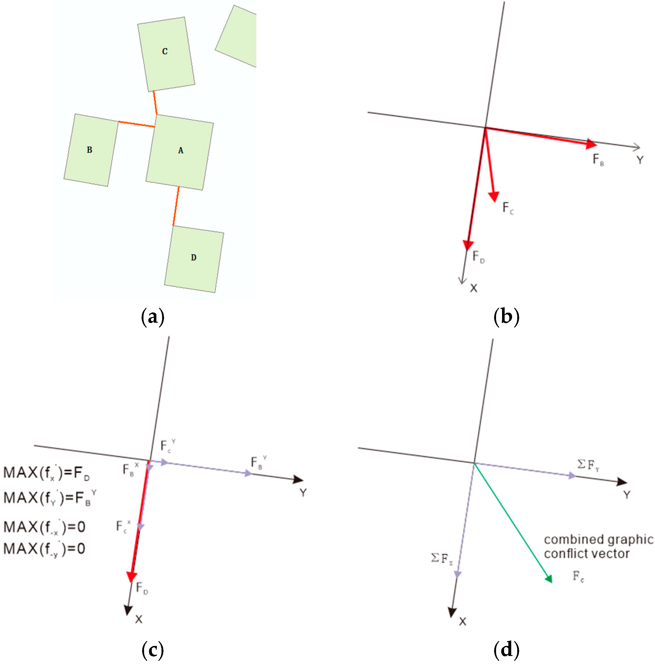
Figure 6.
The initial movement template vector.
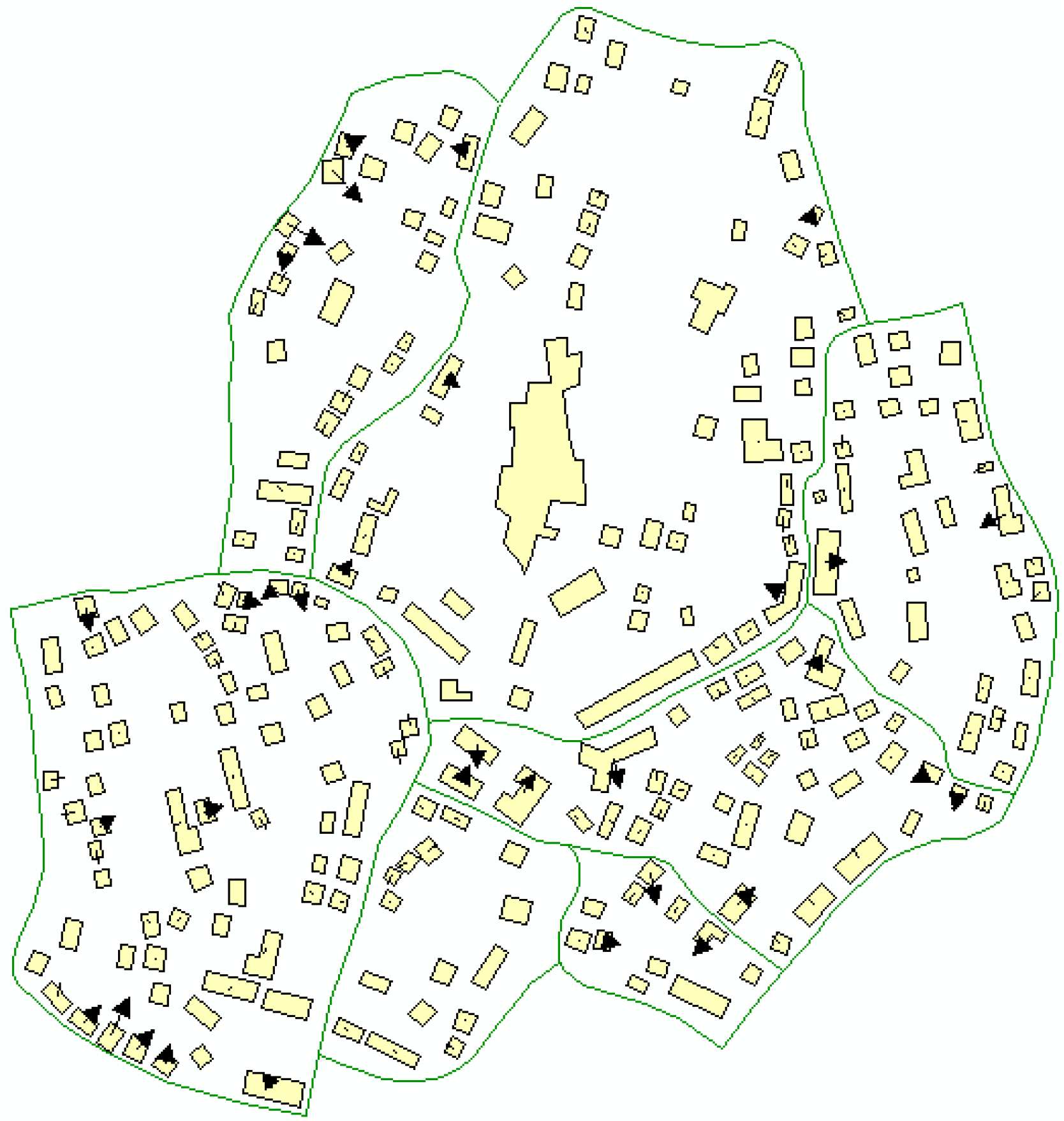
Figure 7.
The crossed velocity is depicted by the orange vector.

Figure 8.
Building conflicts and displacements: (a) The original map with graphic conflicts; (b) the displacement result of the immune genetic algorithm IGA after 10 iterations; (c) the displacement result of IGA after 20 iterations; (d) the displacement result of the improved PSO after 10 iterations; (e) the displacement result of the improved PSO after 20 iterations. (The scale of all five maps is 1:25,000).

Figure 9.
Building displacement results from IGA and the improved PSO: (a) the original buildings close to a road segment; (b) the IGA building displacement result; (c) the improved PSO building displacement result.
Figure 9.
Building displacement results from IGA and the improved PSO: (a) the original buildings close to a road segment; (b) the IGA building displacement result; (c) the improved PSO building displacement result.

Figure 10.
Displacement distance comparison graph (unit: meter).

Figure 11.
Graphic conflict reduction (unit: meter).


Table 1.
Displacement results after 10 iterations.
| Buildings Partition | Building Number | Conflict Number before | IGA (Iteration Number = 10) | Improved PSO (Iteration Number = 10) | ||||
|---|---|---|---|---|---|---|---|---|
| Conflict Number after | Total Displacement Distance (m) | Average Displacement on Map (mm) | Conflict Number after | Total Displacement Distance (m) | Average Displacement Distance on Map (mm) | |||
| 1 | 28 | 26 | 13 | 5.49 | 0.008 | 0 | 2.71 | 0.004 |
| 2 | 60 | 44 | 26 | 42.68 | 0.028 | 1 | 0.03 | 2 × 10⁻⁵ |
| 3 | 69 | 53 | 24 | 141.51 | 0.082 | 2 | 11.18 | 0.006 |
| 4 | 41 | 49 | 20 | 15.75 | 0.015 | 1 | 8.48 | 0.008 |
| 5 | 31 | 28 | 17 | 15.15 | 0.020 | 0 | 3.71 | 0.005 |
| 6 | 16 | 12 | 10 | 0.70 | 0.002 | 2 | 1.62 | 0.004 |
| 7 | 11 | 10 | 7 | 10.93 | 0.040 | 2 | 7.06 | 0.03 |
| sum | 256 | 222 | 117 | 232.21 | 0.036 | 8 | 34.79 | 0.005 |
Table 2.
Displacement results after 15 iterations.
| Buildings Partition | Building Number | Conflict Number before | IGA (Iteration Number = 15) | Improved PSO (Iteration Number = 15) | ||||
|---|---|---|---|---|---|---|---|---|
| Conflict Number after | Total Displacement Distance (m) | Average Displacement on Map (mm) | Conflict Number after | Total Displacement Distance (m) | Average Displacement on Map (mm) | |||
| 1 | 28 | 26 | 10 | 15.31 | 0.021 | 0 | 0.69 | 0.001 |
| 2 | 60 | 44 | 23 | 15.48 | 0.010 | 1 | 0.12 | 8 × 10⁻⁵ |
| 3 | 69 | 53 | 22 | 40.19 | 0.023 | 1 | 20.55 | 0.012 |
| 4 | 41 | 49 | 15 | 3.39 | 0.003 | 1 | 8.54 | 0.008 |
| 5 | 31 | 28 | 13 | 6.28 | 0.008 | 0 | 3.43 | 0.004 |
| 6 | 16 | 12 | 6 | 8.17 | 0.020 | 2 | 1.62 | 0.004 |
| 7 | 11 | 10 | 6 | 9.31 | 0.034 | 2 | 7.00 | 0.025 |
| sum | 256 | 222 | 95 | 98.13 | 0.015 | 7 | 41.95 | 0.007 |
Table 3.
Displacement results after 20 iterations.
| Buildings Partition | Building Number | Conflict Number before | IGA (Iteration Number = 20) | Improved PSO (Iteration Number = 20) | ||||
|---|---|---|---|---|---|---|---|---|
| Conflict Number after | Total Displacement Distance (m) | Average Displacement on Map (mm) | Conflict Number after | Total Displacement Distance (m) | Average Displacement on Map (mm) | |||
| 1 | 28 | 26 | 14 | 7.07 | 0.010 | 1 | 0.90 | 0.001 |
| 2 | 60 | 44 | 32 | 31.25 | 0.021 | 1 | 0.23 | 0.0002 |
| 3 | 69 | 53 | 32 | 13.81 | 0.008 | 3 | 15.89 | 0.009 |
| 4 | 41 | 49 | 19 | 16.56 | 0.016 | 1 | 12.61 | 0.012 |
| 5 | 31 | 28 | 17 | 4.53 | 0.006 | 0 | 3.71 | 0.005 |
| 6 | 16 | 12 | 10 | 13.94 | 0.035 | 1 | 1.62 | 0.004 |
| 7 | 11 | 10 | 7 | 7.21 | 0.026 | 2 | 7.06 | 0.026 |
| sum | 256 | 222 | 131 | 94.37 | 0.015 | 9 | 42.02 | 0.007 |
© 2017 by the authors. Licensee MDPI, Basel, Switzerland. This article is an open access article distributed under the terms and conditions of the Creative Commons Attribution (CC BY) license (http://creativecommons.org/licenses/by/4.0/).
Share and Cite
MDPI and ACS Style
Huang, H.; Guo, Q.; Sun, Y.; Liu, Y. Reducing Building Conflicts in Map Generalization with an Improved PSO Algorithm. ISPRS Int. J. Geo-Inf. 2017, 6, 127. https://0-doi-org.brum.beds.ac.uk/10.3390/ijgi6050127
AMA Style
Huang H, Guo Q, Sun Y, Liu Y. Reducing Building Conflicts in Map Generalization with an Improved PSO Algorithm. ISPRS International Journal of Geo-Information. 2017; 6(5):127. https://0-doi-org.brum.beds.ac.uk/10.3390/ijgi6050127
Chicago/Turabian StyleHuang, Hesheng, Qingsheng Guo, Yageng Sun, and Yuangang Liu. 2017. "Reducing Building Conflicts in Map Generalization with an Improved PSO Algorithm" ISPRS International Journal of Geo-Information 6, no. 5: 127. https://0-doi-org.brum.beds.ac.uk/10.3390/ijgi6050127
Note that from the first issue of 2016, this journal uses article numbers instead of page numbers. See further details here.