A Remote Sensing Algorithm of Column-Integrated Algal Biomass Covering Algal Bloom Conditions in a Shallow Eutrophic Lake

Abstract

Column integrated algal biomass provides a robust indicator for eutrophication evaluation because it considers the vertical variability of phytoplankton. However, most remote sensing-based inversion algorithms of column algal biomass assume a homogenous distribution of phytoplankton within the water column. This study proposes a new remote sensing-based algorithm to estimate column integrated algal biomass incorporating different possible vertical profiles. The field sampling was based on five surveys in Lake Chaohu, a large eutrophic shallow lake in China. Field measurements revealed a significant variation in phytoplankton profiles in the water column during algal bloom conditions. The column integrated algal biomass retrieval algorithm developed in the present study is shown to effectively describe the vertical variation of algal biomass in shallow eutrophic water. The Baseline Normalized Difference Bloom Index (BNDBI) was adopted to estimate algal biomass integrated from the water surface to 40 cm. Then the relationship between 40 cm integrated algal biomass and the whole column algal biomass at various depths was built taking into consideration the hydrological and bathymetry data of each site. The algorithm was able to accurately estimate integrated algal biomass with R² = 0.89, RMSE = 45.94 and URMSE = 28.58%. High accuracy was observed in the temporal consistency of satellite images (with the maximum MAPE = 7.41%). Sensitivity analysis demonstrated that the estimated algal biomass integrated from the water surface to 40 cm has the greatest influence on the estimated column integrated algal biomass. This algorithm can be used to explore the long-term variation of algal biomass to improve long-term analysis and management of eutrophic lakes.

1. Introduction

Inland freshwater ecosystems play an important role in the economic, cultural, aesthetic, scientific and educational aspects of their local and regional populations [1]. However, due to the sharply increasing human demands for freshwater in the past century, inland freshwater ecosystems are globally undergoing increased modification [2,3]. An increased anthropogenic input of nitrogen and phosphorus from agriculture, industrial waste and sewage has caused widespread eutrophication [4,5,6,7]. Affected locations include the Baltic Sea [8], Lake Garda in Italy [9,10], the East China Sea [11], Lake Taihu in China [12], Lake Bogoria in Kenya [13,14], Lake Victoria in Africa [15,16], Lake Erie in the United States [17,18], Lake Michigan in the United States [19,20], Lake Columbia in Canada [21,22], Bahía Blanca Estuary in Argentina [23,24] and the Great Barrier Reef in Australia [25,26]. Inland eutrophication has led to increasing occurrences of cyanobacteria blooms, with impact on water, fisheries and biodiversity [27,28].

Remote sensing has been used to assess eutrophication status with major success. In addition, it is less labor-intensive and time-consuming [29]. Traditional remote sensing provides information on the extent of cyanobacterial blooms [30,31,32,33], the cyanobacterial blooms intensity [30] and pigment concentrations including chlorophyll (Chl-a) [13,34,35,36,37] and phycocyanin [38,39,40]. However, these estimations focus on near-surface investigations, which are not accurate because they do not consider the vertical migration of algae. In reality, some algae (i.e., cyanobacterial) are able to adjust their vertical position within the water column [29,41]. Temperature, light conditions, nutrient availability and interactions with other micro-organisms, grazers and pathogens also have an influence on algae’s vertical migration [42,43,44]. Moreover, the vertical distribution can variate between seasons and algae species [45].

The limited relationship between surface and total column algal biomass has been evidenced by rapid changes observed in remote sensing of surface investigation over a short time. For instance, the bloom area has been observed to double even within 6 h in the East China Sea from Geo-stationary Ocean Color Imager (GOCI) observation [11]. Neither algal growth rate nor environmental conditions would allow bloom areas to expand at such a rapid pace, indicating that vertical migration of algae is a likely cause [46]. Thus, column integrated algal biomass is considered to be a more robust indicator of eutrophication.

Empirical estimation of heterogeneous column-integrated algal biomass is often conducted using in situ measurements, such as the vertical profile of Chl-a. For Case I waters, for example, open sea, where the optical signal is only dominated by phytoplankton and related materials, a Gaussian profile is often observed for profile description [47]. Specific parameters describing the vertical profiles are retrieved from their linkage with surface Chl-a concentrations, remote sensing reflectance and other environmental parameters, such as wind speed [48,49,50]. However, these algorithms are appropriate for Case I waters only, where water leaving reflectance signal is mainly determined by phytoplankton and related breakdown products. Additionally, a large sampling dataset is needed to obtain the profile parameters [8,51]. For Case II waters, that is, coastal and inland waters, the optical signal is more complicated and the influences of phytoplankton, total suspended matter and Colored Dissolved Organic Matter (CDOM) need to be considered [52]. In eutrophicated Case II waters, Chl-a concentration can be extremely high, further complicating the vertical distribution. Past studies have shown that surface information and local physical/hydrologic conditions, such as water depth, influences the vertical profile for Case II waters [53,54]. However, this relationship has been retrieved limited to the non-bloom condition. During algal blooms, higher surface Chl-a concentrations occur, with a sharp decrease of Chl-a concentration, especially for depths below 1 m. An exponential or hyperbolic vertical profile type has been observed, making the use of a Gaussian profile inappropriate due to overestimation of total column-integrated algal biomass.

Estimations of column-integrated algal biomass under algal bloom conditions commonly assumes homogenous mixing within a nutrient-rich upper layer [55]. Integrating surface Chl-a concentrations and a homogenous layer “critical” depth allows for algal biomass estimation. This “critical depth” replaces the mixed layer depth used in the classic assumption (suitable for most of the non-algal bloom conditions). The critical depth can be estimated from surface irradiance and the diffuse attenuation coefficient, which can be further retrieved from satellite observation [55,56,57]. However, the homogeneous layer assumption is not suitable for eutrophic inland lakes, where high variability can occur in the upper 0.1 m [58]. A more comprehensive approach is needed to better estimate column integrated algal biomass under these conditions.

This study focuses on developing a new remote sensing-based algorithm to determine the column integrated algal biomass during algal bloom conditions. Validation was conducted using in situ measurement and image inversion. Sensitivity analysis and comparison with other algorithms were all conducted. The limitations and further applications in column-integrated algal biomass estimation are also discussed.

2. Study Area and Data

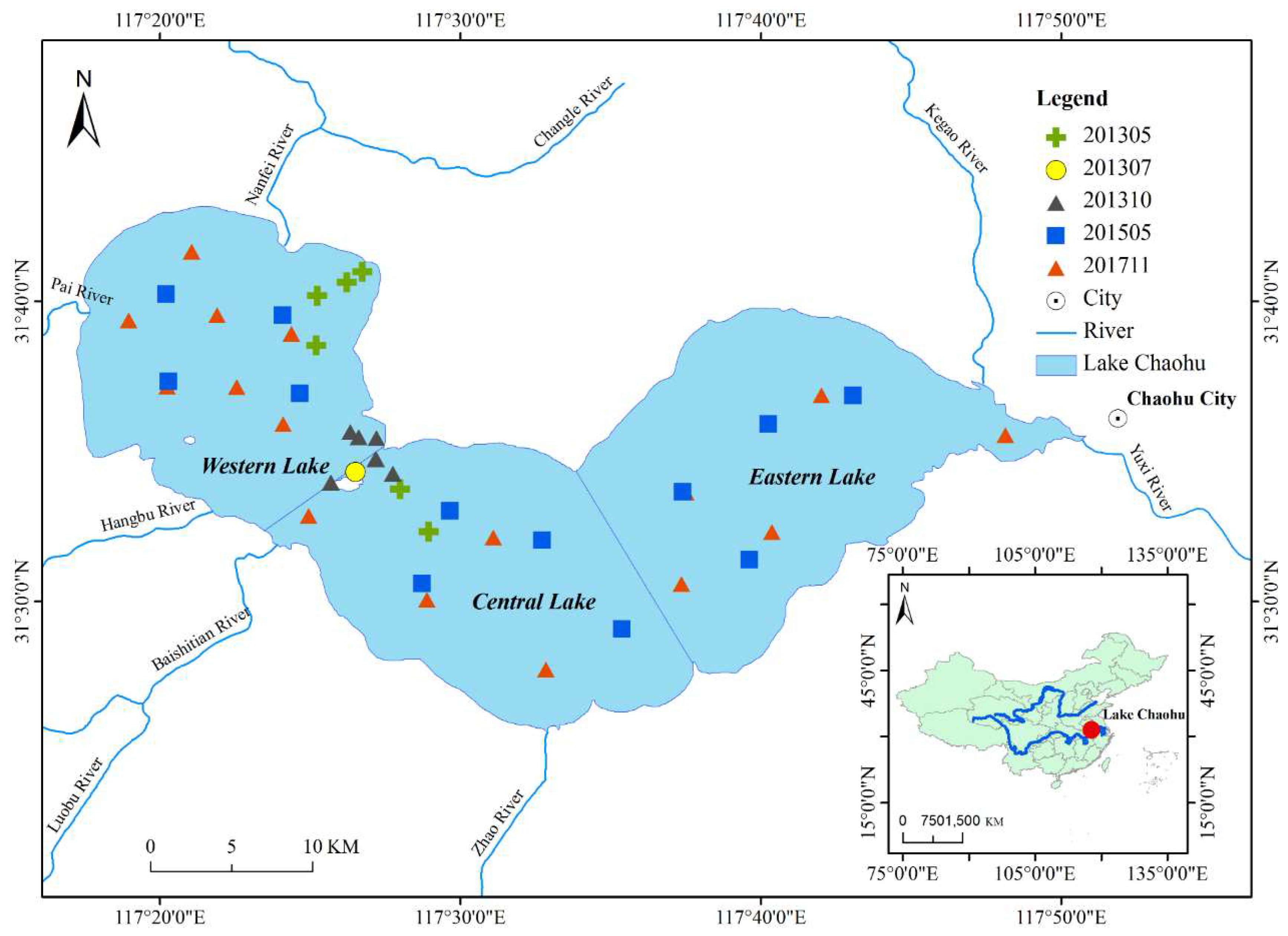
2.1. Study Site

Lake Chaohu is located in Anhui province, the southeast part of China (Figure 1). It is the fifth largest freshwater lake in China, with an average area of 770 km² and a mean water depth of 3.3 m [59,60]. Thirty-three rivers discharges in Lake Chaohu. These rivers belong to seven river systems: the Hangbuhe, the Fenglehe Rivers, the Paihe River, the Nanfei River, the Dianbuhe River, the Baishishanhe River, the Zhegaohe River, the Yuxihe River and the Zhaohe River (Figure 1). The first four rivers contribute more than 90% of the total runoff volume to Lake Chaohu. Finally, the Yuxi River discharges into the Yangtze river [61]. The lake serves as an essential water resource to two large cities, Hefei and Chaohu with nearly 1 million people between them [62]. The lake also plays an important role in tourism and recreation.

The lake has been heavily polluted and suffered from increasing harmful algal blooms since the 1990s. Although several algae species have been observed, cyanobacterial blooms commonly occur from May to November of each year throughout the lake [63,64]. The lake is commonly divided into three parts based on their eutrophication levels; the western part is in severely eutrophic status while the central and eastern parts are considered to be mesotrophic. [65,66].

2.2. In Situ Data

Five surveys were conducted in Lake Chaohu during May, July and October 2013, May 2015 and November 2017 (Figure 1). For each survey, field measurements focused on the vertical distribution of Chl-a concentration and remote sensing reflectance. Water samples to retrieve Chl-a concentrations were collected at nine different depths (surface, 0.1, 0.2, 0.4, 0.7, 1.0, 1.5, 2 and 3 m) using a customized profiling instrument [54]. The instrument consists of four parts: a graduated profiling sampling wire, a small vacuum pump, a connective tube and a portable battery. The graduated profiling sampling wire was used to collect water at specific depths. Surface water was collected directly through the sampling bottle. Water samples were filtered on board using 25-mm Whatman GF/C glass fiber filters (pore size of 1.2 μm) and then stored in darkness at 4 °C until laboratory analysis. Besides water samples, wind speed and direction were also measured by a handheld anemometer. Additionally, cloud conditions were also recorded simultaneously. In total, 54 water samples were collected in specific locations (Figure 1).

Chl-a concentrations ($\mathsf{\mu }$g/L) was measured according to NASA recommended protocols [67]. Filtered water was extracted with 90% acetone for 24 h in the dark at 4 °C before analysis. Chl-a concentrations were calculated using absorbance at 630, 645, 663 and 750 nm measured by a UV-2600 spectrophotometer (Shimadzu Corp., Kyoto, Japan) [68].

Column-integrated algal biomass was calculated based on the nine discrete Chl-a concentrations. For each sampling site, nine depth Chl-a concentrations were evaluated using regression analysis for profile shape: Gaussian, exponential and hyperbolic. Root mean square error and coefficient of determination (R²) for each fitted model were recorded and compared with the Curve Fitting Toolbox of MATLAB R2016a software (The Math Works, Inc., Natick, MA, USA). The fitted model with the lowest RMSE and highest R² (Coefficient of determination) were selected to describe the corresponding vertical profile of Chl-a. Column integrated algal biomass was calculated through the integration of each determined vertical profile. The result has been validated by in situ measurements, with a mean absolute error less than 5%.

2.3. Remote Sensing Data

In situ remote sensing reflectance $R_{rs}$ was measured by the a FieldSpec Pro Dual VNIR (Analytical Spectral Devices, Boulder, CO, USA) following NASA Ocean optics protocols. The instrument has a spectral wavelength range from 350 to 1050 nm. Two probes have a 25-degree field of view. Water leaving radiance $L_t$, the radiance of gray reference panel $L_g$ and sky radiance $L_s$ were measured via this instrument. Under extreme bloom conditions, the algae can be easily disturbed by boat movement. To solve this difficulty, only large and homogenous lake area with algal bloom were selected for field measurement. For these sites, the $R_{rs}$ measurements were conducted 5 times to obtain the average value.

Moderate Resolution Imaging Spectroradiometer (MODIS) 250-m and 500-m resolution Level-0 data from 2003 to 2016 were downloaded from the U.S. NASA Goddard Space Flight Center (http://oceancolor.gsfc.nasa.gov). Level-0 data were processed to calibrated radiance (Level-1B) within SeaDAS software (version 7.0). Rayleigh-correction, which corrected for gaseous absorption and Rayleigh scattering effects, was conducted on Level-1B data. Partial atmospheric correction was used to avoid incorrect data masking when using SeaDAS to do a full atmospheric correction [69]. Over highly turbid coastal and inland waters, saturation of the MODIS ocean band is possible [70]; therefore, we used the terrestrial instead of ocean band.

3. Development of Column-Integrated Algal Biomass Algorithm

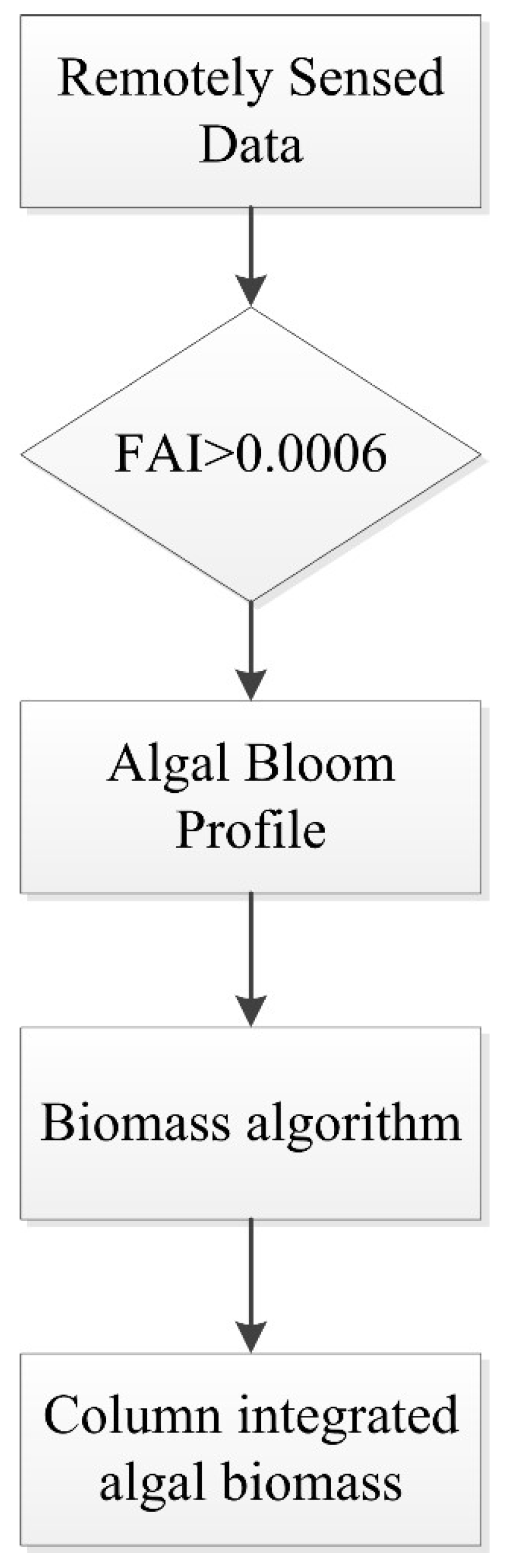
3.1. Algorithm Approach (Flow Chart)

The general approach consisted of a multistep process (Figure 2). MODIS L1b data was processed to determine reflectance R_rc. The floating algae index (FAI) was applied to each satellite image to identify algal bloom conditions for each pixel. FAI has been successfully applied to identify surface bloom in coastal and inland waters under various environmental and observation conditions. For MODIS, FAI was described as:

$$\begin{gathered} \mathrm{FAI}=R_{rc}{}^{\prime }\left(859\right)-R_{rc}\left(859\right) \\ {R}_{rc}{}^{\prime }\left(859\right)=R_{rc}\left(859\right)-\left[R_{rc}\left(1240\right)-R_{rc}\left(645\right)\right]*\left(\left(859-645\right)/\left(1240-645\right)\right) \end{gathered}$$

(1)

where $R_{rc}\left(645\right)$, $R_{rc}\left(859\right)$, $R_{rc}\left(1240\right)$ stands for Rayleigh-corrected reflectance with the central band at 645, 859 and 1240 nm respectively, referring to band 1, band 2 and band 5 for MODIS. Following an earlier study, the time-independent threshold FAI = 0.0006 was adopted to identify algal bloom conditions in Lake Chaohu.

Then, column integrated algal biomass estimation was applied to the extract algal bloom conditions only. An algorithm was built based on an empirical relationship between surface investigation and depth-integrated algal biomass. Parameters to describe the relationship were retrieved from the regression model. Finally, the algorithm was used in combination with the bathymetry data and remote sensing data to estimate column-integrated algal biomass. A more detailed algorithm building process is described in the following paragraph.

3.2. Depth-Integrated Algal Biomass Retrieval from the Surface Investigation

(1) Principles of the algorithm

Based on the field observation, R_rs under algal bloom conditions has two minima around 440 and 625. This was due to the absorption by Chl-a and phycocyanin respectively. Additionally, significantly higher R_rs was also observed at NIR range compared to non-algal bloom conditions. This is contributed by the dense surface phytoplankton under algal bloom conditions. Therefore, bands of blue, red and NIR were considered to characterize the column integrated algal biomass under algal bloom conditions.

The BNDBI index uses a combination of the wave bands that has been shown to accurately estimate algal biomass under algal bloom conditions. The index was built based on the normalized difference of R_rc at 555 nm and a corrected R_rc 645 nm, derived from the baseline by R_rc at 469 nm and 859 nm [71].

BNDBI = [R_rc(555)’ − R_rc(645)’]/[R_rc(555)’ + R_rc(645)’]
R_rc(555)’ = R_rc(555) − [R_rc(469)] × (859 − 555)/(859 − 469) + R_rc(859) × (555 − 469)/(859 − 469)]
R_rc(645)’ = R_rc(645) − [R_rc(469)] × (859 − 645)/(859 − 469) + R_rc(859) × (645 − 469)/(859 − 469)]

(2)

where R_rc(469), R_rc(555), R_rc(645), R_rc(859) are Rayleigh-corrected reflectance with the wavebands centered at 469 nm, 555 nm, 645 nm and 859 nm, corresponding to band 3, band 4, band 1 and band 2 of MODIS, respectively.

The relationship between BNDBI index and Chl-a is nonlinear and the column integrated algal biomass algorithm was developed with a non-linear relationship.

(2) Depth-integrated algal biomass algorithm procedure

Based on sampling results under algal bloom conditions, the relationship between surface information and column integrated algal biomass was retrieved. A high correlation was observed between the Baseline Normalized Difference Bloom Index (BNDBI) and algal biomass present in the surface layers (from the surface to 10, 20 and 40 cm respectively) (Figure 3).

Algal biomass integrated to 40 cm had the highest correlation with the BNDBI index. Hence this layer, surface to 40 cm, was selected to retrieve column algal biomass at other depths. The relationship between BNDBI index and algal biomass integrated to 40 cm (Bio(40))can be described as:

Bio(40) = 4.217 × exp(10.771 × BNDBI)

(3)

As the water depth of Lake Chaohu is less than 6 m, the algorithm was built to include algal biomass up 6 m [54]. A good linear relationship was observed between $Bio\left(40\right)$ and column integrated algal biomass at different depth layers, with R² = 0.81, NRMSD = 0.43. The specific relationship was illustrated in Figure 4a–f). For instance, from the surface to depth of 3 m in Figure 4c, the relationship can be quantified as y = 1.702x + 16.740 with R² of 0.82.

Therefore, the relationship between algal biomass integrated from the surface to 40 cm and column integrated algal biomass can be described as follows:

AI = a × Bio(40) + b

(4)

where AI (mg·m⁻²) is column integrated algal biomass at different water depths. a, b are empirical coefficients related to water depth.

(3) Parameters retrieval

The coefficient a and b were obtained based on in situ measurements. For each sampling depth, the corresponding a and b were estimated following Equation (4) using Matlab (R2015a). For the depths where in situ data were not covered, a linear interpolation was used to estimate the column algal biomass and further derived coefficients a and b (Figure 5). Multiple regression models were tested and the one with maximum R² was adopted. Finally, a log model was selected to derive coefficient a from water depth. The good fitness was ascribed to the shape of Chl-a’s vertical distribution under algal bloom conditions. A linear model was used to describe coefficient b, which is closely related to water depth. The good correlation was attributed to a relatively stable background Chl-a concentration at different depth intervals. The specific relationship between coefficients a and b and water depth can be described as:

a = 0.337 × ln(z) + 1.312
b = 6.453 × z − 2.028

(5)

where z refers to water depth. It was calculated based on hydrological data and DEM data of Lake Chaohu. More details on water depth calculation were described in the previous paper [54].

3.3. Performance Evaluation

The accuracy of algal biomass estimation was evaluated using four statistical indicators: mean absolute percentage error (MAPE), root mean square error (RMSE), unbiased RMSE (URMSE) and normalized root-mean-square deviation (NRMSD):

$$\mathrm{MAPE}=\frac{1}{N}{\displaystyle {\displaystyle \sum }_{i=1}^N}\frac{\left|x_i-y_i\right|}{x_i}\times 100$$

(6)

$$\mathrm{RMSE}=\sqrt{\frac{1}{N}{\displaystyle {\displaystyle \sum }_{i=1}^N}{(x_i-y_i)}^2}$$

(7)

$$\mathrm{URMSE}=\sqrt{\frac{1}{N}{\displaystyle {\displaystyle \sum }_{i=1}^N}(\frac{x_i-y_i}{0.5\times (x_i + y_i)})}$$

(8)

$$\mathrm{NRMSD}=\frac{\sqrt{\frac{1}{N}{\sum }_{i=1}^N{\left(x_i-y_i\right)}^2}}{x_{max}-x_{min}}$$

(9)

where $x_i$ and $y_i$ refer to the measured and estimated values for the ith sample and N is the sample number. URMSE was chosen to avoid deviations by skewed error distributions.

4. Results

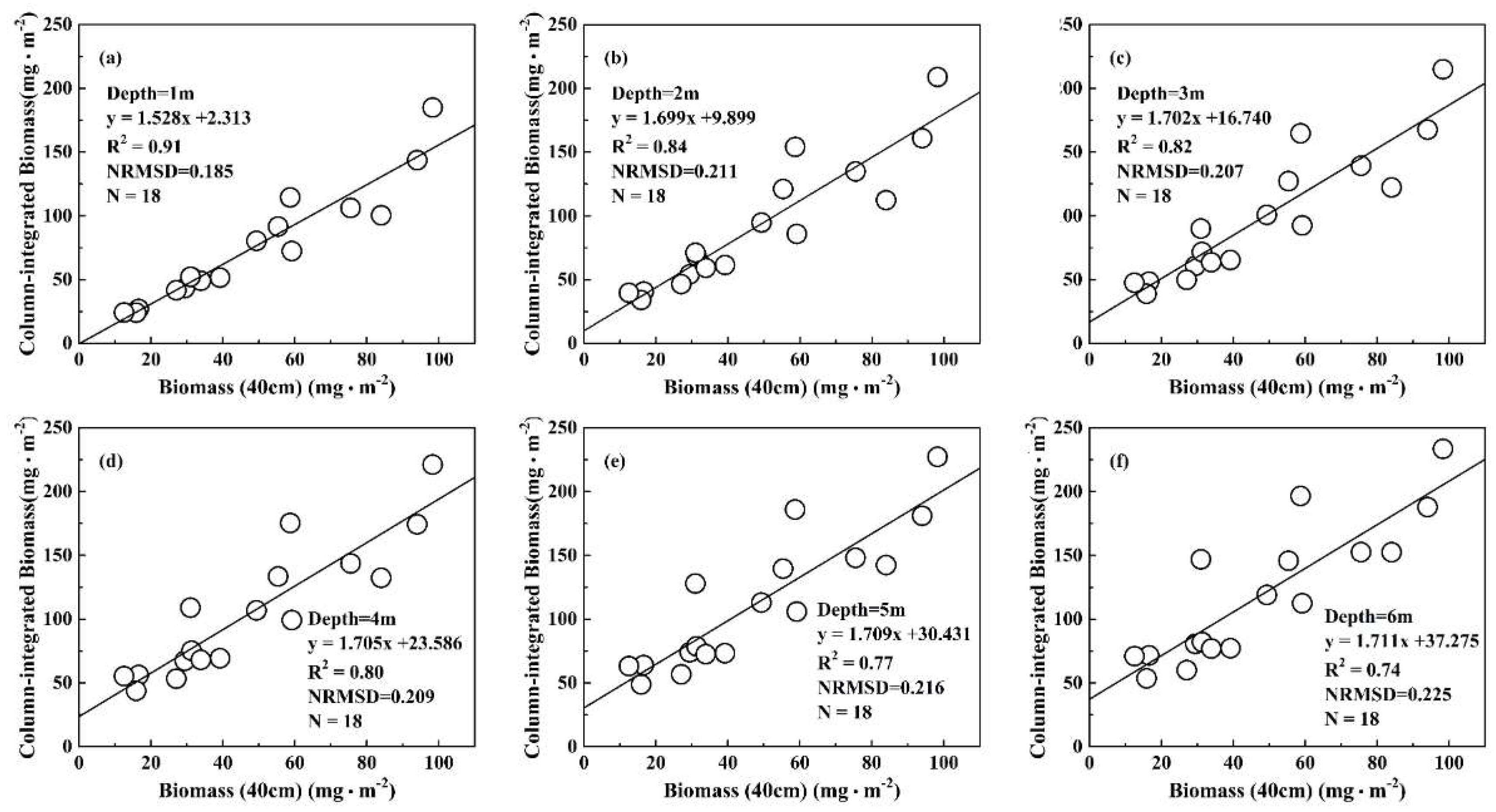
4.1. Field Observation of Column-Integrated Algal Biomass under Algal Bloom Conditions

Chl-a and column integrated algal biomass were retrieved based on the methods mentioned in Section 2.2.

Table 1. Measurements from sampling campaigns in Lake Chaohu from during May, July and October 2013, May 2015 and November 2017: chlorophyll concentration (Chl-a, $\mathsf{\mu }\mathrm{g}/\mathrm{L}$), algal biomass (mg · m⁻²) at each different water depth.

	Chl-a					Algal Biomass
Depth (m)	Mean	Max	Min	SD	CV(%)	Mean	Max	Min	SD	CV(%)
0.1	136.40	313.85	55.43	71.44	52.37	14.82	33.10	5.85	7.51	50.69
0.2	96.70	217.50	24.67	59.73	61.77	11.65	26.57	4.01	6.42	55.09
0.4	70.83	195.62	20.91	43.13	60.89	14.45	33.14	4.54	8.37	57.97
0.7	47.77	113.88	15.20	29.59	61.94	17.79	46.43	6.49	10.54	59.25
1	32.56	90.16	12.39	20.96	64.36	12.05	27.91	4.14	7.29	60.51
1.5	23.52	59.40	6.19	13.93	59.22	14.02	37.39	6.61	8.56	61.08
2	12.95	36.54	3.39	8.88	68.59	9.12	20.97	2.40	5.32	58.39
3	9.31	36.54	3.39	8.42	90.48	11.13	36.54	3.39	8.25	74.12

Note: Algal biomass stands for a 0.1 m integration at the specific depth layer. For instance, algal biomass at 0.2 m refers to algal biomass integrated from 0.15 to 0.25 m.

demonstrated the statistical result of the Chl-a concentration and the corresponding column integrated algal biomass at each depth layer. For instance, Chl-a concentration at 0.2 m is retrieved from field measurement directly, while algal biomass at 0.2 m refers to algal biomass integrated from 0.15 to 0.25 m. Both Chl-a and column integrated algal biomass exhibited large vertical variability. For Chl-a, the maximum concentration was located at the surface layer with the average value of 136.40 $\mathsf{\mu }\mathrm{g}/\mathrm{L}$, with a large range of 55.43 to 313.85 $\mathsf{\mu }\mathrm{g}/\mathrm{L}$. The Chl-a concentration generally decreases with the water depth. For algal biomass, the maximum average value was located around 0.7 m. This demonstrated that higher Chl-a concentration had a weak correlation to increasing algal biomass. Additionally, the CV value of both Chl-a and algal biomass increased with water depth, indicating that the relationship between surface concentrations and those of each layer should be carefully considered. The column integrated algal biomass was used in algorithm validation.

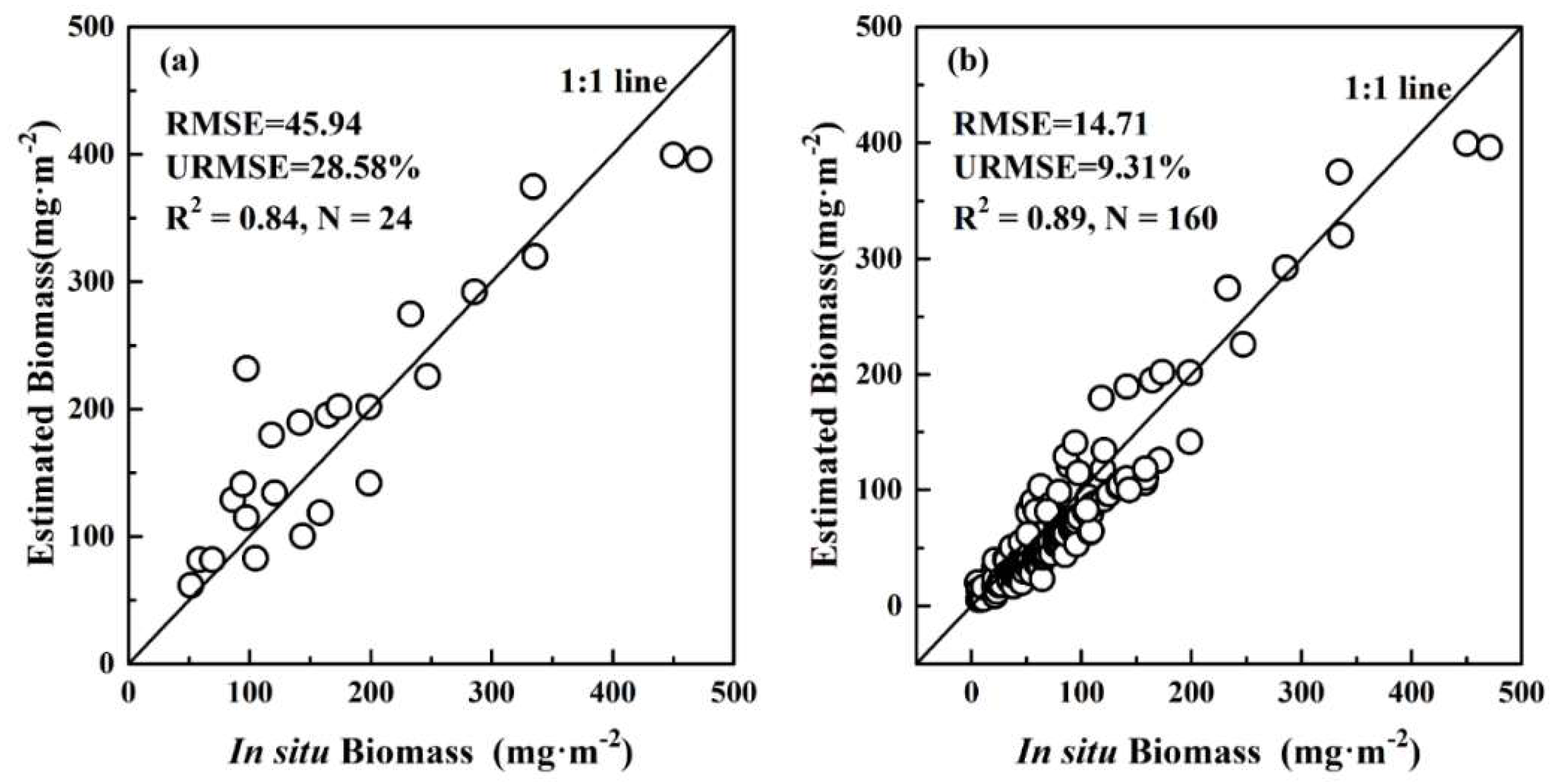
4.2. Algorithm Validation

The algorithm validation was processed in two ways. One is based on the water column validation and the other is based on the temporal consistency of remote sensing images from different time periods. For water column validation, in situ water samples in algal bloom conditions were selected to examine the algorithm’s accuracy. The temporal consistency of satellite derived algal biomass is another effective method of algorithm validation; the total algal biomass should remain consistent over short time periods.

4.2.1. Water Column Validation

Water column validation was conducted comparing in situ measurements and estimations from satellite images. The in situ validation dataset (N = 24) contains column integrated algal biomass and measured water depth under algal bloom conditions. Synchronous satellite data were used to calculate BNDBI index and estimate column algal biomass (Figure 6a). A significant correlation was observed, with R² = 0.84, RMSE = 45.94 and URMSE = 28.58%. For extremely high algal biomass conditions, an underestimation was observed.

Including the validation dataset under non-algal bloom conditions, a high correlation was found with R² = 0.89, RMSE = 14.71 and URMSE = 9.31% (Figure 6b). The result demonstrated that the developed algorithm is quite reliable.

4.2.2. Area-Integrated Validation

This validation method was based on the temporal consistency of satellite images over time. Temporal consistency of algal biomass estimations was also examined by comparing the estimated result from satellite images over different time periods on consecutive days.

Observation from MODIS data on consecutive days demonstrated good consistency (Figure 7a,b). Algal biomass changed from 25.91 t to 23.99 t in February 2004. Satisfying results were obtained with MAPE of 7.41%. Similar results were derived from consecutive images’ observation. Algal biomass on consecutive days ranged from 26.76 t to 28.63 t in May 2016. The variation was 1.87 t with MAPE of 6.98%. A lower error was observed in area integrated algal biomass compared to in situ points. Generally, the high correlation and temporal consistency show the built algorithm was applicable and reliable for both in situ and satellite data.

4.3. Sensitivity Analysis

A sensitivity analysis was conducted to observe which parameters have the greatest impact on the results. A simulation was conducted by a HydroLight radiative transfer model with highly variable integrated column algal biomass while keeping all other input parameters constant. Based on in situ datasets (see Table 1), two input parameters, Bio(40) and depth, were modified by $\pm$5%, $\pm$10% and $\pm$20%, respectively based on the average value. Bio(40) was found to have greater influence than depth in algal biomass calculation under algae bloom conditions (

Table 2. Sensitivity analysis of the total algal biomass algorithm under algal bloom conditions.

Total Algal Biomass Variation (%)
Parameter variation	5%	10%	20%
Bio(40)	4.10	8.20	16.41
z	1.03	2.05	4.07

). When Bio(40) was altered by $\pm$20%, the calculated algal biomass was $\pm$16.41%, while in term of depth, the corresponding variation was only $\pm$4.07%. Thus, the algorithm was less sensitive to depth than algal biomass integrated from the surface to 40 cm. This revealed different results under non-algal bloom conditions, where surface investigation was less sensitive to water depth [54].

5. Discussion

5.1. Comparison with Other Algorithms

Three proposed algorithms were evaluated and compared with our algorithm using the in situ validation dataset. The comparison result was illustrated in

Table 3. Comparison of the performance of the column integrated algal biomass algorithm applied to the in situ dataset from the present study.

Algorithms	R2	RMSE	URMSE(100%)	Reference
MB89	0.6204	278.9908	0.8503	[72]
Uitz proposed	0.6201	599.0637	1.1607	[49]
Critical depth based	0.0721	252.8243	1.6160	[57]
This study	0.84	45.94	0.2858	--

. For the Morel and Uitz algorithms, the in situ surface Chl-a concentration data was used directly to estimate the column integrated algal biomass at each site. For the Chriswell algorithm, the calculation of “critical depth,” derived from the diffuse attenuation coefficient (K_d), surface irradiance and equivalence irradiance (where depth production equals losses), was not measured in our field surveys. Therefore, we used the radiative transfer model—HydroLight—to simulate these parameters. The input parameters (including Chl-a vertical concentration, SPIM, CDOM, absorption coefficient etc.) were kept the same as in the field measurements.

Morel’s algorithms (in short for MB89 here below) were built based on nearly 4000 vertical profiles of Chl-a in ocean water only [72]. In this dataset, most maximum Chl-a concentrations were typically located in the subsurface, which can be more than two orders different from the surface layer. This is not consistent with the vertical profile in lake water under algal bloom conditions, where the maximum Chl-a value is in the surface layer. Therefore, the overestimation of MB89 resulted in a RMSE = 278.9908, URMSE = 0.8503. However, a good correlation was observed, as the MB89 algorithm is based on the theory that the integrated algal biomass and the near-surface Chl-a concentration are highly but nonlinearly related. Our algorithm is also based on similar observations. Therefore, a good correlation was observed when applying MB89 to our dataset with the R² = 0.6204. The result was retrieved following the Utiz algorithm. The overestimation from the Utiz algorithm results from a variable background Chl-a value applied to replace the constant background value. The depth variable background value was derived from the surface concentration with a linear relationship. Due to the much higher surface Chl-a in lake water than ocean water, a larger background Chl-a was estimated, resulting in a large overestimation.

For the critical depth-based algorithm, surface Chl-a concentration is a key input parameter. The much higher surface Chl-a concentration commonly leads to an extremely high algal biomass value at each water column. This also made the estimated value more discrete and resulted in the observation of the lowest R².

Comparing to other algorithms, our algorithm performs best with R² = 0.84, RMSE = 45.94, URMSE = 0.2858.

5.2. Analysis of Variation in Spatial Distribution

The seasonal changes in spatial distribution variation are attributed to the succession of dominant algae species. Three main algae species observed in Lake Chaohu were: Cyanobacteria, Bacillariophytes and Chlorophytes. A high abundance of Cyanobacteria was observed in summer, which contributes to the heavy cyanobacterial bloom [62]. Starting in the autumn, cyanobacterial blooms degrade and are replaced by Bacillariophytes and Chlorophytes. Bacillariophytes are dominant in later winter and spring. Chlorophytes is the dominant species in spring and autumn. Moreover, Bacillariophytes and Chlorophytes are observed to be higher in the east lake segment of Lake Chaohu [73].

According to Figure 6a,b, a nearly homogeneous spatial distribution was observed in Lake Chaohu. This is because the dominant algae species is Bacillariophytes during this time was evenly distributed in the lake. In May, higher algal biomass was observed in the east lake driven by Chlorophytes. In Figure 6c,d, a growing trend could be observed in the west lake, showing the increasing Cyanobacteria concentrations, which lead to high spatial variation between the west lake and other segments.

5.3. Extension and Application of the Algorithm

5.3.1. Extending Application to other Lakes

When applying this algorithm to other lakes, such as Lake Taihu, two points should be noted. First, the threshold of FAI index used to identify the algal bloom conditions should be recalculated. This FAI threshold is based on a long time series of statistics and can be different from one lake to another [30,54]. The algorithm is applied for algal bloom conditions only. Therefore, the accurate threshold may have an influence on the inversion result. The other factor is the specific coefficients in the algorithm. Even if the algorithm from Equations (2) and (4) can be applied to other lakes, the specific coefficients need to be adjusted (or validated) using local sampled data, as the coefficients in this study were determined from empirical regression with the Lake Chaohu dataset. The composition of in-water optical constituents may vary between lakes, which will lead to various different vertical distributions of phytoplankton [38].

5.3.2. Algorithm for Data from Other Sensors

The most significant strength of the algorithm comes from its use of green and red MODIS bands (band 1 and band 4). These broad wavebands allow the algorithm to be applied to other satellite systems (such as Landsat, Sentinel and SPOT). In theory, the algorithm could be applied to datasets with different temporal or spatial resolution when an appropriate atmospheric correction is conducted. In particular, the algorithm can be applied to the ocean and coastal sensors, such as ESA’s Sentinel-3 OLCI and NASA’s planned hyperspectral Plankton-Aerosol-Cloud-ocean Ecosystem (PACE)’s primary sensor, the Ocean Color Instrument (OCI). All of these missions will provide chances to further develop, refine and validate the algorithm to retrieve more accurate inversion results.

5.4. Algorithm Limitations

Our algorithm illustrated robust estimation of column-integrated algal biomass under algal bloom conditions. However, the algorithm may have problems in extremely high bloom conditions. In the validation process, points with surface Chl-a concentration over 700 ($\mathsf{\mu }$g/L) were removed. Usually, under such conditions, cyanobacteria floats on the surface and accumulates to form scums [74]. The corresponding remote sensing reflectance is similarly observed with terrestrial plants, rather than water [32]. Large overestimation may occur if the built algorithm is applied. For this extreme condition, additional measurement and algorithm development is needed.

Another challenge in applying the algorithm is the difference in spatial resolution and the temporal gap between satellite and field measurements. Satellite data have a spatial coverage (i.e., MODIS has 250 m resolution) that may not be completely covered by algal bloom. Differences in local environmental factors, may also lead to differences in the vertical migration of algae. Furthermore, a temporal gap may exist between satellite data and field measurements, leading to an error when calibrating the algorithm.

6. Conclusions

The remote sensing-based algorithm to retrieve the column algal biomass in shallow eutrophic lakes under algal bloom condition was developed and validated by both in situ measurements and spatial consistency from the inversion of satellite images. Validation results demonstrated the algorithm is quite reliable and stable for Lake Chaohu. Sensitivity analysis showed the most sensitive input parameters involved algal biomass integrated from the water surface to 40 cm. The limitations and further applications were also discussed.

This algorithm allows the estimation of the vertical variability of phytoplankton in the eutrophic shallow lakes under algae bloom conditions. Except for extremely conditions, when surface Chl-a concentrations is over 700 ($\mathsf{\mu }$g/L). In general, the algorithm will ultimately improve the monitoring of algal biomass variability and eutrophication status, providing new, more accurate information for lake management.

References

1. Dudgeon, D.; Arthington, A.H.; Gessner, M.O.; Kawabata, Z.-I.; Knowler, D.J.; Lévêque, C.; Naiman, R.J.; Prieur-Richard, A.-H.; Soto, D.; Stiassny, M.L. Freshwater biodiversity: Importance, threats, status and conservation challenges. Boil. Rev. 2006, 81, 163–182. [Google Scholar] [CrossRef] [PubMed]
2. Strayer, D.L.; Dudgeon, D. Freshwater biodiversity conservation: Recent progress and future challenges. J. N. Am. Benthol. Soc. 2010, 29, 344–358. [Google Scholar] [CrossRef]
3. Schindler, D.W. Recent advances in the understanding and management of eutrophication. Limnol. Oceanogr. 2006, 51, 356–363. [Google Scholar] [CrossRef] [Green Version]
4. Smith, V.H. Eutrophication of freshwater and coastal marine ecosystems a global problem. Environ. Sci. Pollut. Res. 2003, 10, 126–139. [Google Scholar] [CrossRef]
5. Paerl, H.W.; Otten, T.G. Harmful cyanobacterial blooms: Causes, consequences, and controls. Microb. Ecol. 2013, 65, 995–1010. [Google Scholar] [CrossRef] [PubMed]
6. Dodds, W.K.; Smith, V.H. Nitrogen, phosphorus, and eutrophication in streams. Inland Waters 2016, 6, 155–164. [Google Scholar] [CrossRef]
7. Padisák, J.; Reynolds, C.S. Shallow lakes: The absolute, the relative, the functional and the pragmatic. Hydrobiologia 2003, 506, 1–11. [Google Scholar] [CrossRef]
8. Hunter, P.D.; Matthews, M.W.; Kutser, T.; Tyler, A.N. Remote Sensing of Cyanobacterial Blooms in Inland, Coastal, and Ocean Waters. In Handbook of Cyanobacterial Monitoring and Cyanotoxin Analysis; John Wiley & Sons: Hoboken, NJ, USA, 2016; pp. 89–99. [Google Scholar]
9. Brivio, P.; Giardino, C.; Zilioli, E. Determination of chlorophyll concentration changes in Lake Garda using an image-based radiative transfer code for Landsat TM images. Int. J. Remote Sens. 2001, 22, 487–502. [Google Scholar] [CrossRef]
10. Giardino, C.; Brando, V.E.; Dekker, A.G.; Strömbeck, N.; Candiani, G. Assessment of water quality in Lake Garda (Italy) using Hyperion. Remote Sens. Environ. 2007, 109, 183–195. [Google Scholar] [CrossRef]
11. Lou, X.; Hu, C. Diurnal changes of a harmful algal bloom in the East China Sea: Observations from GOCI. Remote Sens. Environ. 2014, 140, 562–572. [Google Scholar] [CrossRef]
12. Duan, H.; Ma, R.; Hu, C. Evaluation of remote sensing algorithms for cyanobacterial pigment retrievals during spring bloom formation in several lakes of East China. Remote Sens. Environ. 2012, 126, 126–135. [Google Scholar] [CrossRef]
13. Tebbs, E.; Remedios, J.; Harper, D. Remote sensing of chlorophyll-a as a measure of cyanobacterial biomass in Lake Bogoria, a hypertrophic, saline–alkaline, flamingo lake, using Landsat ETM+. Remote Sens. Environ. 2013, 135, 92–106. [Google Scholar] [CrossRef]
14. Omondi, R.; Yasindi, A.; Magana, A. Spatial and temporal variations of zooplankton in relation to some environmental factors in Lake Baringo, Kenya. Egerton J. Sci. Technol. 2015, 11, 29–50. [Google Scholar]
15. Hecky, R. The eutrophication of lake Victoria. Int. Ver. Theor. Angew. Limnol. Verh. 1992, 25, 39–48. [Google Scholar] [CrossRef]
16. Mbonde, A.S.; Sitoki, L.; Kurmayer, R. Phytoplankton composition and microcystin concentrations in open and closed bays of Lake Victoria, Tanzania. Aquat. Ecosyst. Health Manag. 2015, 18, 212–220. [Google Scholar] [CrossRef] [PubMed] [Green Version]
17. Scavia, D.; Allan, J.D.; Arend, K.K.; Bartell, S.; Beletsky, D.; Bosch, N.S.; Brandt, S.B.; Briland, R.D.; Daloğlu, I.; DePinto, J.V. Assessing and addressing the re-eutrophication of Lake Erie: Central basin hypoxia. J. Great Lakes Res. 2014, 40, 226–246. [Google Scholar] [CrossRef] [Green Version]
18. Kane, D.D.; Conroy, J.D.; Richards, R.P.; Baker, D.B.; Culver, D.A. Re-eutrophication of Lake Erie: Correlations between tributary nutrient loads and phytoplankton biomass. J. Great Lakes Res. 2014, 40, 496–501. [Google Scholar] [CrossRef]
19. LaBuhn, S.; Klump, J.V. Estimating summertime epilimnetic primary production via in situ monitoring in an eutrophic freshwater embayment, Green Bay, Lake Michigan. J. Great Lakes Res. 2016, 42, 1026–1035. [Google Scholar] [CrossRef]
20. Sawyers, J.E.; McNaught, A.S.; King, D.K. Recent and historic eutrophication of an island lake in northern Lake Michigan, USA. J. Paleolimnol. 2016, 55, 97–112. [Google Scholar] [CrossRef]
21. Kulkarni, A. Water quality retrieval from Landsat TM imagery. Procedia Comput. Sci. 2011, 6, 475–480. [Google Scholar] [CrossRef]
22. Cumming, B.F.; Laird, K.R.; Gregory-Eaves, I.; Simpson, K.G.; Sokal, M.A.; Nordin, R.; Walker, I.R. Tracking past changes in lake-water phosphorus with a 251-lake calibration dataset in British Columbia: Tool development and application in a multiproxy assessment of eutrophication and recovery in Osoyoos Lake, a transboundary lake in Western North America. Front. Ecol. Evol. 2015, 3, 84. [Google Scholar]
23. Spetter, C.V.; Popovich, C.A.; Arias, A.; Asteasuain, R.O.; Freije, R.H.; Marcovecchio, J.E. Role of nutrients in phytoplankton development during a winter diatom bloom in a eutrophic South American estuary (Bahía Blanca, Argentina). J. Coast. Res. 2013, 31, 76–87. [Google Scholar] [CrossRef]
24. Guinder, V.; Popovich, C.; Perillo, G. Phytoplankton and physicochemical analysis on the water system of the temperate estuary in South America: Bahía Blanca Estuary, Argentina. Int. J. Environ. Res. 2012, 6, 547–556. [Google Scholar]
25. Brodie, J.; Devlin, M.; Haynes, D.; Waterhouse, J. Assessment of the eutrophication status of the Great Barrier Reef lagoon (Australia). Biogeochemistry 2011, 106, 281–302. [Google Scholar] [CrossRef]
26. Blondeau-Patissier, D.; Schroeder, T.; Brando, V.E.; Maier, S.W.; Dekker, A.G.; Phinn, S. ESA-MERIS 10-year mission reveals contrasting phytoplankton bloom dynamics in two tropical regions of Northern Australia. Remote Sens. 2014, 6, 2963–2988. [Google Scholar] [CrossRef]
27. Otten, T.G.; Crosswell, J.R.; Mackey, S.; Dreher, T.W. Application of molecular tools for microbial source tracking and public health risk assessment of a Microcystis bloom traversing 300 km of the Klamath River. Harmful Algae 2015, 46, 71–81. [Google Scholar] [CrossRef]
28. Meneely, J.P.; Elliott, C.T. Microcystins: Measuring human exposure and the impact on human health. Biomarkers 2013, 18, 639–649. [Google Scholar] [CrossRef] [PubMed]
29. Hunter, P.; Tyler, A.; Willby, N.; Gilvear, D. The spatial dynamics of vertical migration by Microcystis aeruginosa in a eutrophic shallow lake: A case study using high spatial resolution time—Series airborne remote sensing. Limnol. Oceanogr. 2008, 53, 2391–2406. [Google Scholar] [CrossRef]
30. Hu, C.; Lee, Z.; Ma, R.; Yu, K.; Li, D.; Shang, S. Moderate resolution imaging spectroradiometer (MODIS) observations of cyanobacteria blooms in Taihu Lake, China. J. Geophys. Res. Oceans 2010, 115. [Google Scholar] [CrossRef]
31. Wynne, T.; Stumpf, R.; Tomlinson, M.; Warner, R.; Tester, P.; Dyble, J.; Fahnenstiel, G. Relating spectral shape to cyanobacterial blooms in the Laurentian Great Lakes. Int. J. Remote Sens. 2008, 29, 3665–3672. [Google Scholar] [CrossRef]
32. Gower, J.; Doerffer, R.; Borstad, G. Interpretation of the 685 nm peak in water-leaving radiance spectra in terms of fluorescence, absorption and scattering, and its observation by MERIS. Int. J. Remote Sens. 1999, 20, 1771–1786. [Google Scholar] [CrossRef]
33. Gower, J.; King, S.; Borstad, G.; Brown, L. Detection of intense plankton blooms using the 709 nm band of the MERIS imaging spectrometer. Int. J. Remote Sens. 2005, 26, 2005–2012. [Google Scholar] [CrossRef]
34. Matthews, M.W.; Bernard, S.; Robertson, L. An algorithm for detecting trophic status (chlorophyll-a), cyanobacterial-dominance, surface scums and floating vegetation in inland and coastal waters. Remote Sens. Environ. 2012, 124, 637–652. [Google Scholar] [CrossRef]
35. Li, L.; Li, L.; Song, K. Remote sensing of freshwater cyanobacteria: An extended IOP Inversion Model of Inland Waters (IIMIW) for partitioning absorption coefficient and estimating phycocyanin. Remote Sens. Environ. 2015, 157, 9–23. [Google Scholar] [CrossRef]
36. Ogashawara, I.; Moreno-Madriñán, M.J. Improving inland water quality monitoring through remote sensing techniques. ISPRS Int. J. Geo-Inf. 2014, 3, 1234–1255. [Google Scholar] [CrossRef]
37. Ha, N.T.T.; Thao, N.T.P.; Koike, K.; Nhuan, M.T. Selecting the Best Band Ratio to Estimate Chlorophyll-a Concentration in a Tropical Freshwater Lake Using Sentinel 2A Images from a Case Study of Lake Ba Be (Northern Vietnam). ISPRS Int. J. Geo-Inf. 2017, 6, 290. [Google Scholar] [CrossRef]
38. Qi, L.; Hu, C.; Duan, H.; Cannizzaro, J.; Ma, R. A novel MERIS algorithm to derive cyanobacterial phycocyanin pigment concentrations in a eutrophic lake: Theoretical basis and practical considerations. Remote Sens. Environ. 2014, 154, 298–317. [Google Scholar] [CrossRef]
39. Randolph, K.; Wilson, J.; Tedesco, L.; Li, L.; Pascual, D.L.; Soyeux, E. Hyperspectral remote sensing of cyanobacteria in turbid productive water using optically active pigments, chlorophyll a and phycocyanin. Remote Sens. Environ. 2008, 112, 4009–4019. [Google Scholar] [CrossRef]
40. Gorham, T.; Jia, Y.; Shum, C.; Lee, J. Ten-year survey of cyanobacterial blooms in Ohio’s waterbodies using satellite remote sensing. Harmful Algae 2017, 66, 13–19. [Google Scholar] [CrossRef]
41. Hu, L.; Hu, C.; Ming-Xia, H. Remote estimation of biomass of Ulva prolifera macroalgae in the Yellow Sea. Remote Sens. Environ. 2017, 192, 217–227. [Google Scholar] [CrossRef]
42. Reynolds, C.S.; Oliver, R.L.; Walsby, A.E. Cyanobacterial dominance: The role of buoyancy regulation in dynamic lake environments. N. Z. J. Mar. Freshw. Res. 1987, 21, 379–390. [Google Scholar] [CrossRef] [Green Version]
43. Walsby, A.; Utkilen, H.; Johnsen, I. Buoyancy changes of a red coloured Oscillatoria agardhii in Lake Gjersjoen, Norway. Arch. Hydrobiol. 1983, 97, 18–38. [Google Scholar]
44. Walsby, A.; Schanz, F. Light—Dependent growth rate determines changes in the population of Planktothrix rubescens over the annual cycle in Lake Zürich, Switzerland. New Phytol. 2002, 154, 671–687. [Google Scholar] [CrossRef]
45. Walsby, A.E. Stratification by cyanobacteria in lakes: A dynamic buoyancy model indicates size limitations met by Planktothrix rubescens filaments. New Phytol. 2005, 168, 365–376. [Google Scholar] [CrossRef] [PubMed]
46. Qi, L.; Hu, C.; Visser, P.M.; Ma, R. Diurnal changes of cyanobacteria blooms in Taihu Lake as derived from GOCI observations. Limnol. Oceanogr. 2018, 63, 1711–1726. [Google Scholar] [CrossRef] [Green Version]
47. Sathyendranath, S.; Prieur, L.; Morel, A. A three-component model of ocean colour and its application to remote sensing of phytoplankton pigments in coastal waters. Int. J. Remote Sens. 1989, 10, 1373–1394. [Google Scholar] [CrossRef]
48. Frolov, S.; Ryan, J.; Chavez, F. Predicting euphotic-depth-integrated chlorophyll-afrom discrete-depth and satellite-observable chlorophyll-a off central California. J. Geophys. Res. Oceans 2012, 117. [Google Scholar] [CrossRef]
49. Uitz, J.; Claustre, H.; Morel, A.; Hooker, S.B. Vertical distribution of phytoplankton communities in open ocean: An assessment based on surface chlorophyll. J. Geophys. Res. Oceans 2006, 111. [Google Scholar] [CrossRef] [Green Version]
50. Lewis, M.R.; Cullen, J.J.; Platt, T. Phytoplankton and thermal structure in the upper ocean: Consequences of nonuniformity in chlorophyll profile. J. Geophys. Res. Oceans 1983, 88, 2565–2570. [Google Scholar] [CrossRef]
51. Odermatt, D.; Gitelson, A.; Brando, V.E.; Schaepman, M. Review of constituent retrieval in optically deep and complex waters from satellite imagery. Remote Sens. Environ. 2012, 118, 116–126. [Google Scholar] [CrossRef] [Green Version]
52. Moore, G.; Aiken, J.; Lavender, S. The atmospheric correction of water colour and the quantitative retrieval of suspended particulate matter in Case II waters: Application to MERIS. Int. J. Remote Sens. 1999, 20, 1713–1733. [Google Scholar] [CrossRef]
53. Nouchi, V.; Odermatt, D.; Wüest, A.; Bouffard, D. Effects of non-uniform vertical constituent profiles on remote sensing reflectance of oligo-to mesotrophic lakes. Eur. J. Remote Sens. 2018, 51, 808–821. [Google Scholar] [CrossRef]
54. Li, J.; Zhang, Y.; Ma, R.; Duan, H.; Loiselle, S.; Xue, K.; Liang, Q. Satellite-based estimation of column-integrated algal biomass in nonalgae bloom conditions: A case study of Lake Chaohu, China. IEEE J. Sel. Top. Appl. Earth Obs. Remote Sens. 2017, 10, 450–462. [Google Scholar] [CrossRef]
55. Matsumoto, K.; Honda, M.C.; Sasaoka, K.; Wakita, M.; Kawakami, H.; Watanabe, S. Seasonal variability of primary production and phytoplankton biomass in the western Pacific subarctic gyre: Control by light availability within the mixed layer. J. Geophys. Res. Oceans 2014, 119, 6523–6534. [Google Scholar] [CrossRef] [Green Version]
56. Sverdrup, H. On conditions for the vernal blooming of phytoplankton. J. Cons. 1953, 18, 287–295. [Google Scholar] [CrossRef]
57. Chiswell, S.M. Annual cycles and spring blooms in phytoplankton: Don’t abandon Sverdrup completely. Mar. Ecol. Prog. Ser. 2011, 443, 39–50. [Google Scholar] [CrossRef]
58. Xue, K.; Zhang, Y.; Duan, H.; Ma, R.; Loiselle, S.; Zhang, M. A remote sensing approach to estimate vertical profile classes of phytoplankton in a eutrophic lake. Remote Sens. 2015, 7, 14403–14427. [Google Scholar] [CrossRef]
59. Chen, J.; Quan, W. An improved algorithm for retrieving chlorophyll-a from the Yellow River Estuary using MODIS imagery. Environ. Monit. Assess. 2013, 185, 2243–2255. [Google Scholar] [CrossRef]
60. Yin, H.; Deng, J.; Shao, S.; Gao, F.; Gao, J.; Fan, C. Distribution characteristics and toxicity assessment of heavy metals in the sediments of Lake Chaohu, China. Environ. Monit. Assess. 2011, 179, 431–442. [Google Scholar] [CrossRef]
61. Jiang, Y.-J.; He, W.; Liu, W.-X.; Qin, N.; Ouyang, H.-L.; Wang, Q.-M.; Kong, X.-Z.; He, Q.-S.; Yang, C.; Yang, B. The seasonal and spatial variations of phytoplankton community and their correlation with environmental factors in a large eutrophic Chinese lake (Lake Chaohu). Ecol. Indic. 2014, 40, 58–67. [Google Scholar] [CrossRef]
62. Zhang, Y.; Ma, R.; Zhang, M.; Duan, H.; Loiselle, S.; Xu, J. Fourteen-year record (2000–2013) of the spatial and temporal dynamics of floating algae blooms in Lake Chaohu, observed from time series of MODIS images. Remote Sens. 2015, 7, 10523–10542. [Google Scholar] [CrossRef]
63. Cai, Y.; Kong, F.; Shi, L.; Yu, Y. Spatial heterogeneity of cyanobacterial communities and genetic variation of Microcystis populations within large, shallow eutrophic lakes (Lake Taihu and Lake Chaohu, China). J. Environ. Sci. 2012, 24, 1832–1842. [Google Scholar] [CrossRef]
64. Jiang, Y.; Cheng, B.; Liu, M.; Nie, Y. Spatial and temporal variations of taste and odor compounds in surface water, overlying water and sediment of the Western Lake Chaohu, China. Bull. Environ. Contam. Toxicol. 2016, 96, 186–191. [Google Scholar] [CrossRef] [PubMed]
65. Yu, L.; Kong, F.; Zhang, M.; Yang, Z.; Shi, X.; Du, M. The dynamics of Microcystis genotypes and microcystin production and associations with environmental factors during blooms in Lake Chaohu, China. Toxins 2014, 6, 3238–3257. [Google Scholar] [CrossRef]
66. Zhou, Y.; Jin, J.; Liu, L.; Zhang, L.; He, J.; Wang, Z. Inference of reference conditions for nutrient concentrations of Chaohu Lake based on model extrapolation. Chin. Geogr. Sci. 2013, 23, 35–48. [Google Scholar] [CrossRef]
67. Mueller, J.L.; Fargion, G.S.; McClain, C.R.; Pegau, S.; Zanefeld, J.; Mitchell, B.G.; Kahru, M.; Wieland, J.; Stramska, M. Ocean Optics Protocols for Satellite Ocean Color Sensor Validation, Revision 4, Volume IV: Inherent Optical Properties: Instruments, Characterizations, Field Measurements and Data Analysis Protocols; Aeronautics and Space Administration of USA: Greenbelt, MD, USA, 2003.
68. Welschmeyer, N.A. Fluorometric analysis of chlorophyll a in the presence of chlorophyll b and pheopigments. Limnol. Oceanogr. 1994, 39, 1985–1992. [Google Scholar] [CrossRef] [Green Version]
69. Qi, L.; Hu, C.; Duan, H.; Barnes, B.B.; Ma, R. An EOF-based algorithm to estimate chlorophyll a concentrations in Taihu Lake from MODIS land-band measurements: Implications for near real-time applications and forecasting models. Remote Sens. 2014, 6, 10694–10715. [Google Scholar] [CrossRef]
70. Franz, B.A.; Werdell, P.J.; Meister, G.; Kwiatkowska, E.J.; Bailey, S.W.; Ahmad, Z.; McClain, C.R. MODIS land bands for ocean remote sensing applications. In Proceedings of the Ocean Optics XVIII, Montreal, QC, Canada, 9–13 October 2006. [Google Scholar]
71. Zhang, Y.; Ma, R.; Duan, H.; Loiselle, S.; Zhang, M.; Xu, J. A novel MODIS algorithm to estimate chlorophyll a concentration in eutrophic turbid lakes. Ecol. Indic. 2016, 69, 138–151. [Google Scholar] [CrossRef]
72. Morel, A.; Berthon, J.F. Surface pigments, algal biomass profiles, and potential production of the euphotic layer: Relationships reinvestigated in view of remote-sensing applications. Limnol. Oceanogr. 1989, 34, 1545–1562. [Google Scholar] [CrossRef] [Green Version]
73. Deng, D.G.; Xie, P.; Zhou, Q.; Yang, H.; Guo, L.G. Studies on temporal and spatial variations of phytoplankton in Lake Chaohu. J. Integr. Plant Boil. 2007, 49, 409–418. [Google Scholar] [CrossRef]
74. Wynne, T.T.; Stumpf, R.P.; Tomlinson, M.C.; Dyble, J. Characterizing a cyanobacterial bloom in western Lake Erie using satellite imagery and meteorological data. Limnol. Oceanogr. 2010, 55, 2025–2036. [Google Scholar] [CrossRef]
Figure 1. Lake Chaohu, China and the Western, Central and Eastern parts. In situ measurements were conducted in five surveys on 28 May 2013 (N = 6), 24 July 2013 (N = 2), 10–12 October 2013 (N = 25), 25 May 2015 (N = 12) and 27 November 2017 (N = 9). The blue lines in the small frame show the Yangtze and Huang river.
Ijgi 07 00466 g001
Figure 2. Schematic of the processing procedure of column-integrated algal biomass estimation.
Ijgi 07 00466 g002
Figure 3. The relationship between BNDBI index and algal biomass integrated from the surface to different water depth. (ac) refers to the depth of 10, 20, 40 cm respectively. (e.g., in (c), Y-axis refers to algal biomass integrated from surface to 40 cm).
Ijgi 07 00466 g003
Figure 4. The relationship between algal biomass integrated from surface to 40 cm and total algal biomass integrated from surface to various depth based on in situ measurements. (af) represent depth from 1 to 6 m respectively (e.g., in (e), column-integrated algal biomass refers to algal biomass integrated from the surface to 6 m).
Ijgi 07 00466 g004
Figure 5. The relationship between (a) coefficient a, (b) coefficient b and water depth. The black line refers to the fitting line. The corresponding formulas are shown in each figure.
Ijgi 07 00466 g005
Figure 6. Validation results between in situ measured algal biomass and estimated algal biomass from MODIS observation. (a) results under algal bloom conditions; (b) results under all bloom and non-bloom conditions.
Ijgi 07 00466 g006
Figure 7. Area integrated validation results based on satellite images. Estimated algal biomass results from MODIS observation in consecutive days: (a) on 15 February 2004 (b) on 16 February 2004. The variation between (a,b) is 1.08 t with MAPE = 7.41%. Comparison of MODIS derived algal biomass in the adjacent day: (c) on 15 May 2016 (d) on 19 May 2016. The variation is 1.87 t, MAPE = 7.41%.
Ijgi 07 00466 g007