1. Introduction
The main point of this paper is the creation of a 3D model of buildings, using stereoscopic images and control points. The 3D reconstruction of building façades has become an important task for different applications, such as architectural design, cultural heritage, urban planning, cadaster, and virtual tourism. Building façades differ in their structures, shapes and geometries. On one hand, there are historical buildings in old cities, and on the other hand, there are large modern buildings with different architectural designs. The continuous expansion and renewal of cities results in the need for process automation for the buildings documentation.
A number of façade reconstruction methods are based on close-range images or terrestrial laser data [
1]. Close-range photogrammetry has been used to produce heritage building façade maps [
2] for the documentation of historical buildings [
3] and for architectural documentation [
4]. The terrestrial laser point cloud has been extensively used to collect large datasets. Laser scanning technology is a widely accepted and frequently used method for 3D reconstruction. LiDAR (light detection and ranging) has revolutionized mapping for close-range objects [
5]. It has been used for highly-detailed city models and façade reconstruction [
6]. An approach based on the segmentation of building façades using terrestrial laser data is described in [
7]. An automatic extraction of building features from laser-scanned data is presented in [
8]. In recent years there have been approaches that create dense 3D models of exteriors of historical buildings [
9]. Most existing state-of-the-art 3D model reconstruction approaches use 3D laser scanner technology as an increasingly important tool in the fields of archaeological survey and restoration work [
10,
11]. However, the weakness of this method lies in the cost of the equipment and the post-processing needed in order to arrive at the final reconstruction. The raw data from the laser scanner cannot be directly processed and referenced to a geographical coordinated system. To do so, existing approaches utilize a method called registration which is semi-automated in most cases [
12,
13]. The reasoning behind semi-automation lies in the limitations of laser scanning. The technology is highly susceptible to the existence of gaps along laser points. These gaps can lead to reconstruction distortions manifested in the form of offsets between the represented and the actual positions of the structure’s edges. Moreover, to obtain photorealistic results, textures must be mapped from images to the geometric models [
14]. An accurate alignment between the laser space and image space is required which is semi-automatic. Moreover, laser-based methods are constrained by the requirement of large amounts of data points to produce accurate reconstructions. Even so, despite the density of the laser-produced point clouds they often create inconsistencies between the laser and image spaces, leading to texture mapping discontinuities. Laser-based systems are also susceptible to surface material-induced distortions in the form of reflections from glass surfaces and moving objects, thus requiring further data processing in order to counteract them and increase the reconstruction accuracy. To resolve these limitations and obstacles, various approaches have been proposed which combine laser and image sensor data [
15,
16,
17]. The idea behind such methods is that image data can be used to enrich the laser-driven depth information by extracting semantic information from the ground view images in the form of texture and morphological information [
18,
19]. For this task, well-studied machine learning and image processing techniques have been used to determine structural information cues of the structure/building, such as its basic skeleton or boundary information, through morphological operations or edge and contour extraction techniques, and then, combine them with a laser-driven 3D reconstruction of the model [
19,
20]. Combining these data sources has proven to result to an increase in reconstruction accuracy, as well as a broadening of the reconstruction capabilities for a variety of structures [
21,
22,
23].
In the existing 3D building reconstruction approaches, only a few approaches attempt to do it fully automatically [
24]. The reason can be traced back to the complexity of the methods and their requirements/constraints, as well as the structural variety amongst structures. In multimodal methods, the complexity lies in relating the different data sources accurately. The reconstruction methods rely on special targets/key points measured from each scan position with a total station in a ground coordinate system as a means of relating the two coordinate systems. In an automated approach these targets can be found automatically using radiometric and geometric information. Other approaches use key points extracted from the reflection data of the scans for the automatic marker-free registration of terrestrial laser scans [
25]. There is also an approach using image-based assistance to the total stations to empower the surveying instrumentation [
26]. In essence, laser-based approaches cannot be considered ideal for reconstruction due to equipment cost and reconstruction limitations.
In addition, Structure from Motion is proposed to solve some of these problems. Structure from Motion [
27] extracts sparse depth point-clouds that are combined with laser sensor [
28,
29,
30] or georeferenced data [
26,
31,
32] to construct the final 3D model of the structure. However, the performance of Structure from Motion architectures depends highly on the viewing positions and the presence of a sufficient number of common points between each view (large number) in order to be able to relate the different views. Additionally, in Structure from Motion only the interior information of the sensors is considered and, thus, the resulting depth maps are more susceptible to projection errors.
Our method proposes a solution using terrestrial surveying techniques and stereoscopic data of the structure. For that purpose we use common total stations and low cost CCD cameras. We compensate the low-cost, highly-available equipment with sophisticated post-processing. Specifically, in our approach we initially create a point cloud which can be georeferenced using a set of control points obtained by a total station. The point cloud is then enriched with morphological information derived from the image data using image processing methods and a registration process between the two coordinate systems. Moreover, the use of two cameras on the same rig provides us with an image-driven depth of the scene and a second image view of the structure. We only utilize the image-driven depth maps of close range viewing cases where the depth information is accurate enough to approximate structural information about the façade details of the structure/building.
In our approach, the multimodal information is combined into a reconstruction model suitable to be imported in the Unity 3D game engine to create the final 3D model of the viewed structure. Unity 3D is a game development platform, developed by Unity Technologies, that is widely used in architectural visualization by introducing the necessary framework to realistically render 3D content. The provided illumination effects, along with texture mapping, simulate real lighting conditions, enhancing the photorealism of the scene. Our approach was tested in a highly-textured historical building in Chania, Crete, as well as in a homogeneously-textured modern building on the campus of the Technical University of Crete. As a remark we would like to mention that all prior data processing and modeling stages were implemented in Matlab.
In
Section 2 the proposed approach is presented in more detail with a special focus on the methodology applied in order to extract meaningful and useful information from the multimodal sensors.
Section 3 presents the coordinate system registration process that enables the relation of the multimodal datasets.
Section 4 presents results and additional comments on the limitations and constraints of the proposed approach. Finally,
Section 5 offers conclusions and proposes future work for addressing the limitations and constraints of the approach.
2. Proposed Method
The proposed method aims to reconcile data requirements and reconstruction accuracy for accurate building façade 3D reconstruction by fusing multimodal information. Our approach combines information from image sensors and ground control points with the goal of reducing the complexity of the model reconstruction by discarding the dependency of depth information from laser-based systems [
15,
16,
28,
29,
30]. The presented approach is an extension to our previous work [
31] on the specific topic.
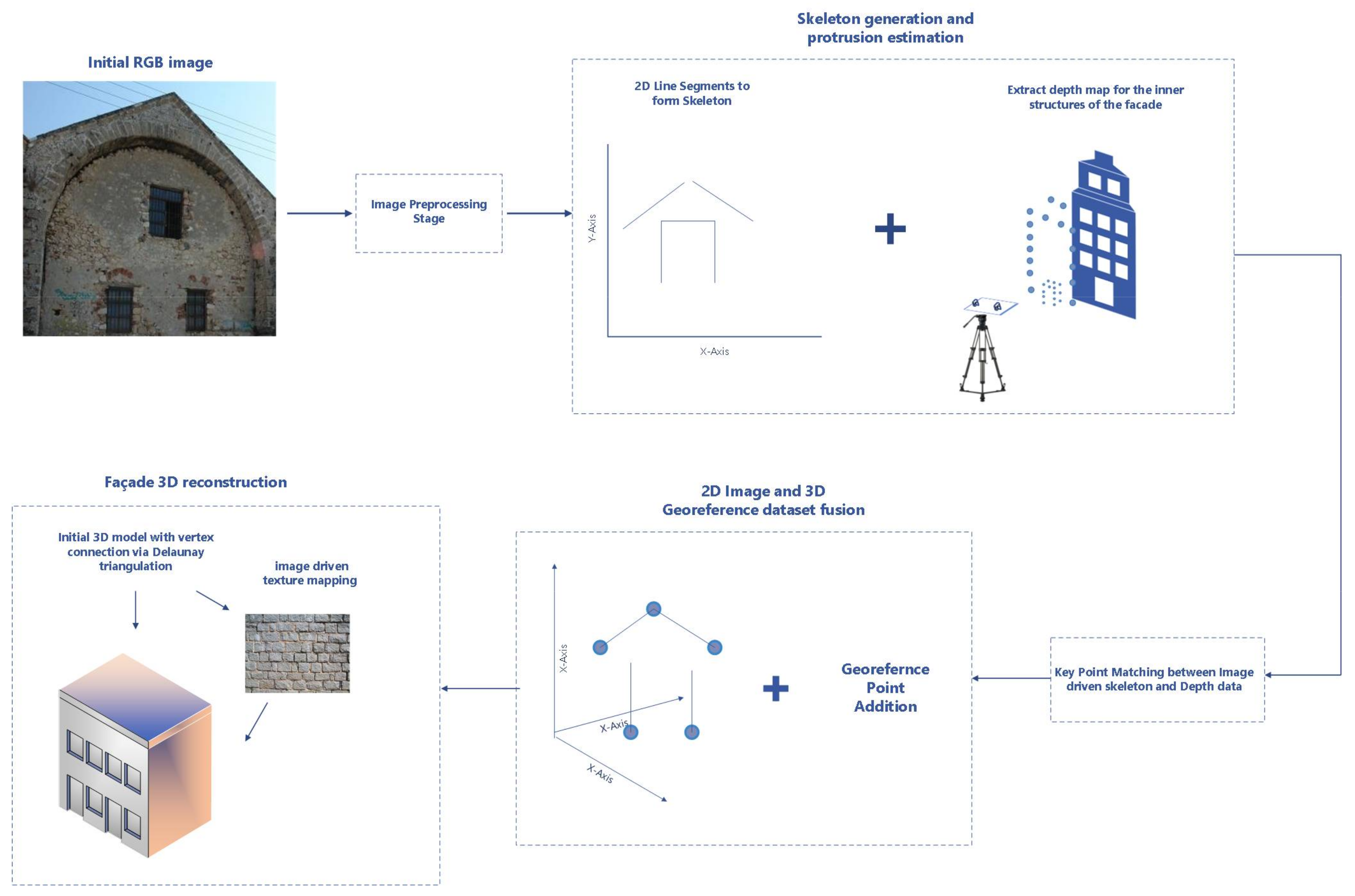
In the first stage of our approach the outer-skeleton of a mosaic building view, is extracted using morphological image processing methods. Subsequently, in the second stage, the 2D skeleton is transformed to a georeferenced 3D point cloud by relating the georeferenced point datasets of the building. This stage will essentially produce the basis for an initial crude 3D building model. Finally, the model is further refined through the addition of depth information for the building’s inner façade features (e.g., windows or doors) that have been extracted from depth point clouds. The overall process of our approach is depicted in
Figure 1. As two examples we use an archeological monument called “Neoria”, located in the old port of Chania and a building on the campus of the University called “campus building”.
The key contributions of the presented scheme concern the introduction of a pre-processing stage which extends the capabilities of our approach on wider structures, as well as the enrichment of the building extraction and 2D building skeleton extraction stages. More specifically, the contributions include (a) the incorporation of a multi-view approach, expanding the viewed structure scene, (b) a more elaborate color segmentation approach, that results in accurate structure isolation/segmentation from the background, and (c) a multi-stage contour extraction refinement scheme, compared to the one introduced in [
31], for the 2D building skeleton process. In the following sections, we will present the components of our approach emphasizing the key features of the methodology, introducing the new contributions and commenting on assumptions and constraints that were used.
2.1. Stereoscopic Camera Layout
We begin by presenting our image acquisition equipment, which is a non-convergent stereoscopic layout consisting of two high-resolution CCD cameras (Prosilica GC1020) facing each side of the structure. The role of the stereoscopic layout is that it allows the extraction of a depth-map estimate for the examined structure.
The use of a stereoscopic camera layout enables the extraction of the depth map of the scene through the relation of the 2D image planes with the 3D scene coordinate systems, a process known as triangulation. The accuracy of the depth estimates depend upon many factors, such as the camera parameters, the camera-object distance, as well as the morphology of the monitored scene (i.e., structural complexity of objects being present) and the monitoring conditions (illumination effects and weather conditions). In order to achieve the best depth estimation accuracy we follow a calibration approach [
33] that enables the estimation of the camera related parameters (interior and exterior). These parameters enable the correction of distortions (lens distortion), up to similarity reconstructions, that preserve line parallelism, angles, and ratios of volume and length. However, in long-range image monitoring, a necessity for building with large dimensions, the reprojection errors increase as the camera-object distance increases [
33,
34]. These reprojection errors lead to ambiguous depth estimates that for the case of 3D building façade models tend to be more severe in the outer structure of the building. The degrading depth information quality due to the increase of the camera-object distance will lead to inaccuracies in the reconstructed model. Nevertheless, we can still retrieve information about the inner building façade features, such as windows or doors, in the form of protrusion indices which can be used in the reconstruction process, a process briefly presented in
Section 2.5.
In the case of old buildings and structures, whose structure or shapes do not satisfy the necessary constraints, we have difficulties in the accurate and meaningful depth estimation from the stereoscopic layout. In such cases, we may fail on the estimation of the protrusion of inner façade structures, but we are still able to produce a 3D approximate reconstruction of the façade, relying on the 2D image and the georeferenced datasets. The subsequent subsections illustrate the steps to extract relevant information from these data sources.
2.2. Image Stitching and Building Extraction
2.2.1. Multiple View Relation and Image Stitching
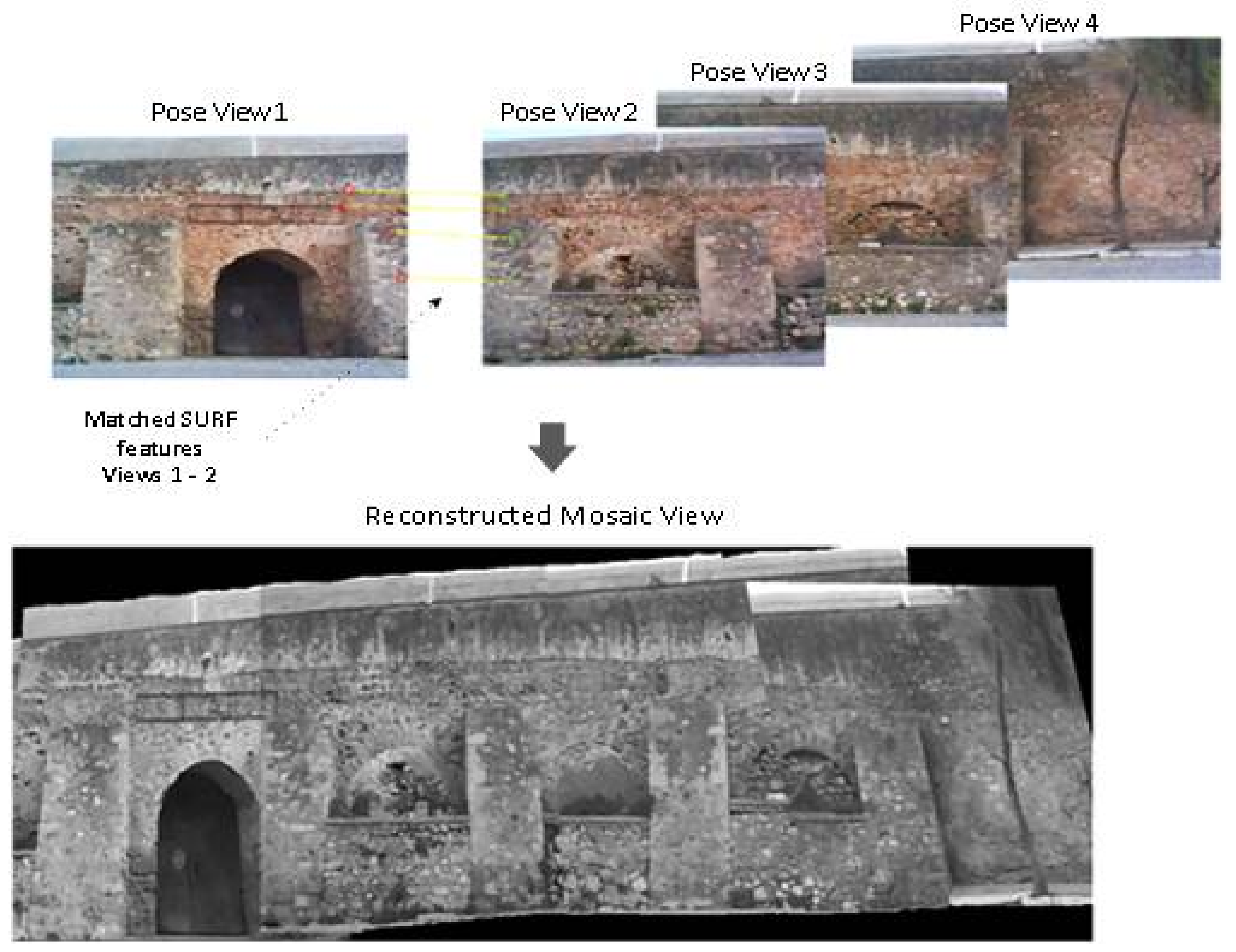
In order to cope with wider structure cases, where the field of the camera is not able to capture the entire façade, we have adopted a mosaic view reconstruction approach. The mosaic reconstruction approach allows for multiple views of the structure to be stitched together to create a single 2D image view of the entire structure [
20]. We employ hierarchic image view pairs of the structure using a Speeded Up Robust Features-based matching (SURF, [
35]). The extracted feature vectors (SURF features) that characterize each view (image) are compared with the goal of deriving a projective transformation that enables the relation of the views into a single image. In order for this method to produce accurate results a sufficient amount of common key points (i.e., portions of a commonly-viewed object) must exist in the examined image pair. By relating adjacent views we can produce a mosaic view of the entire building façade. Please note that this stage is unrelated with the stereo-driven depth map estimation process. We do not attempt to stitch together 3D depth point clouds. Our experiments showed that the results are extremely vulnerable to reprojection errors. The mosaic image is just used to produce a uniform 2D skeleton for longer structures that cannot be represented in total with a single image.
Moreover, in order to produce as accurate as possible mosaic representations of the view we kept a constant viewing distance from the building, while covering the whole building. For example, the Neoria building required a minimum distance of 8 m. The overall process is depicted in
Figure 2, for the case of the historical building of Neoria. Please note that the depicted view is on a grayscale to fulfil the requirements of the contour extraction algorithm that is used in the subsequent stages of the method. This process is still applied prior to the building segmentation stage. Only for better visualization of the stitching results we provide a segmented grayscale view of the mosaic.
Commenting on the specific test case, of the building Neoria, we can observe that, despite the fact that image views were acquired from slightly different viewing distances from the building’s façade, the resulting mosaic view preserves the structural alignment of the building’s façade. However, small alignment errors still exist mainly on the rooftop of the building. Please note that these errors occur due to (a) the uneven structure of the roads surrounding the building and, (b) that the building, itself, is built in an uphill location. As a final remark, please note that the mosaic view, as well as the entire skeleton extraction process, is applied on the restored (undistorted) view of the left camera, whose color information is adjusted with respect to the view of the right camera.
2.2.2. Color-Based Building Extraction
The next stage involves preprocessing of the image data that results in the segmentation of the image and the extraction of the building. For this task, as presented in our previous work [
31], we utilize a color-based segmentation scheme, applied on the transformed version of the image in the LAB color space, that separates the 2D image into a background class (the sky) and a foreground class (the structure). This is an effective yet simple approach whose success requires the structure to have homogeneous color shades. This constraint, however, is easily violated in outdoor conditions due to extreme illumination.
In order to solve this problem, we apply the mean shift color segmentation method [
36] using a six-class scheme. The mosaic view is decomposed into different regions based on the color distribution characteristics of the pixels, under the assumption that the textural information of the building is coherent within its structural limits.
The extraction of the building from the surrounding object classes is achieved by first merging neighboring classes with similar color characteristics (thresholding on the difference of the mean color values of two classes) and then selecting the class containing the largest amount of points. The only assumption is that the components of the structure are coherent in texture, in order to ensure that the building’s structural details and boundaries are retained.
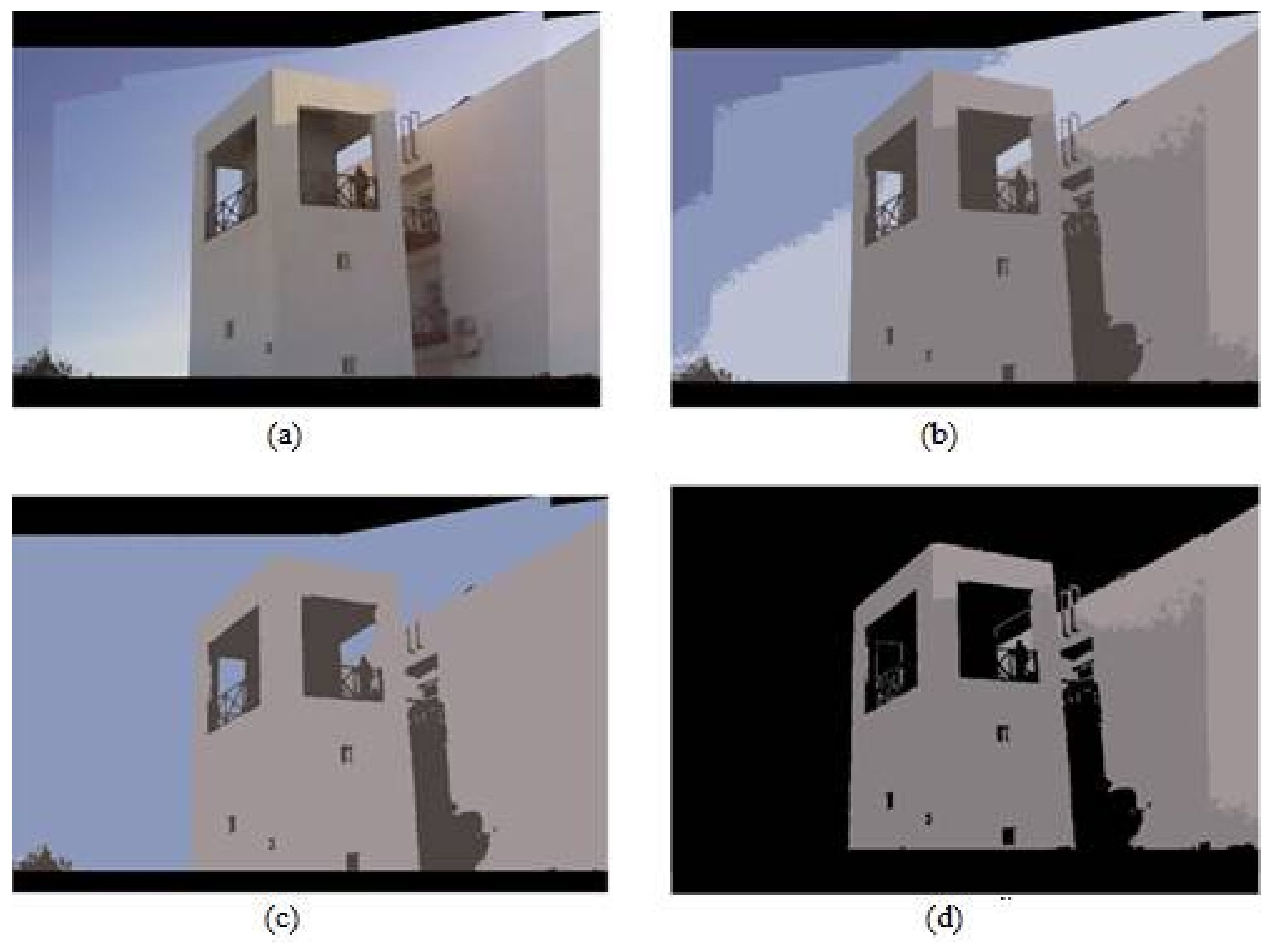
Figure 3 depicts the extraction process in one of our case studies: the campus building.
2.3. Building Skeleton Extraction
Following the preprocessing stage (mosaic view formation, building extraction), we proceed to the extraction of the 2D structural skeleton of the building. This process involves the application of morphological operations, as well as edge detection and ‘significant’ line extraction on the segmented mosaic view of the building. The goal of this stage is two-fold, first to extract the 2D skeleton and, second, to detect and extract the building’s inner structural details, such as windows, doors, or ledges. The latter is achieved through the application of shape-based morphological filtering methods.
2.3.1. Building Façade Contour Extraction
The 2D skeleton extraction is essentially the process of extracting the building’s contour. Following the method presented in our earliest work [
31], we apply the Canny edge detector approach [
37], followed by an Active Contour process [
38] that leads to the final contour of the building. The Canny edge detector serves as a closed contour initialization process that produces an early form of the building’s structural skeleton. In order to cope with unexpected effects on the captured image, such as shadows and intensity deterioration along the building this contour estimate is refined with the use of a more elaborate active contour tracing methods [
38].
The Active Contour model is a curve fitting approach in which the curve properties are guided by an energy minimization scheme that consists of two factors; the internal forces (smoothness term) which control the model’s smoothness and generalization during the deformation process, and external forces (data term) which describe the fitting of the curve in the data, i.e., the objects of the image.
The only requirement is that an initial contour H0 close to a valid contour of the image must be provided (which in our case is provided by the Canny edge estimate) in order for the method to search for possible deformations of the H0 that can lead to the actual contour of the structure.
Finally, in order to cope with large structures, as well as to ensure that the contour captures the majority of the structural characteristics of the building, we sequentially apply the active contour extraction process on several edge points in the image, iteratively examining the curve relaxation condition, where we are looking for the next possible position of the curve. More specifically we start with a closed curve and iteratively modify them by applying shrink or expansion operations performed by the minimization of the energy function, which consist of internal forces (defined by constraints upon the shape of the contour) and external forces (defined by gradient). In that way, we can also ensure that structural and textural deformations do not randomly affect the guidance of a single spline, leading to local convergence issues and thus, to erroneous estimates.
2.3.2. Building Skeleton Formulation
The next stage of our process is the generation of an initial 2D structural skeleton of the building by fitting distinct line segments on the extracted edges through the application of the Hough line transformation method [
39,
40]. As expected, the fitting accuracy depends on the accuracy of the edge-based representation of the building’s contour and inner structural details (doors, windows, etc.). This process, however, can be affected by various factors. In structures with non-homogeneous textures, such as Neoria, shown in
Figure 1, image mapping distortions, due to uneven illumination, can lead to the detection of erroneous and unwanted edge segments. In such cases, noisy line segments are produced that reduce the accuracy of the 2D structural skeleton.
Another factor that affects the overall accuracy is the parameterization of the edge detection process. Depending on the threshold selected in the Canny edge detection stage, the number and strength of the extracted line segments can vary significantly. In our earliest work [
31], we argued that the sequential application of the edge detection and line segment extraction processes, by varying the values of their parameters, increases the line segment 2D skeleton description performance. Higher thresholds preserve only the basic morphology of the structure, whereas smaller thresholds retain information about the inner structural details. However, using smaller thresholds can lead to the preservation of erroneous edges that inaccurately describe the structure.
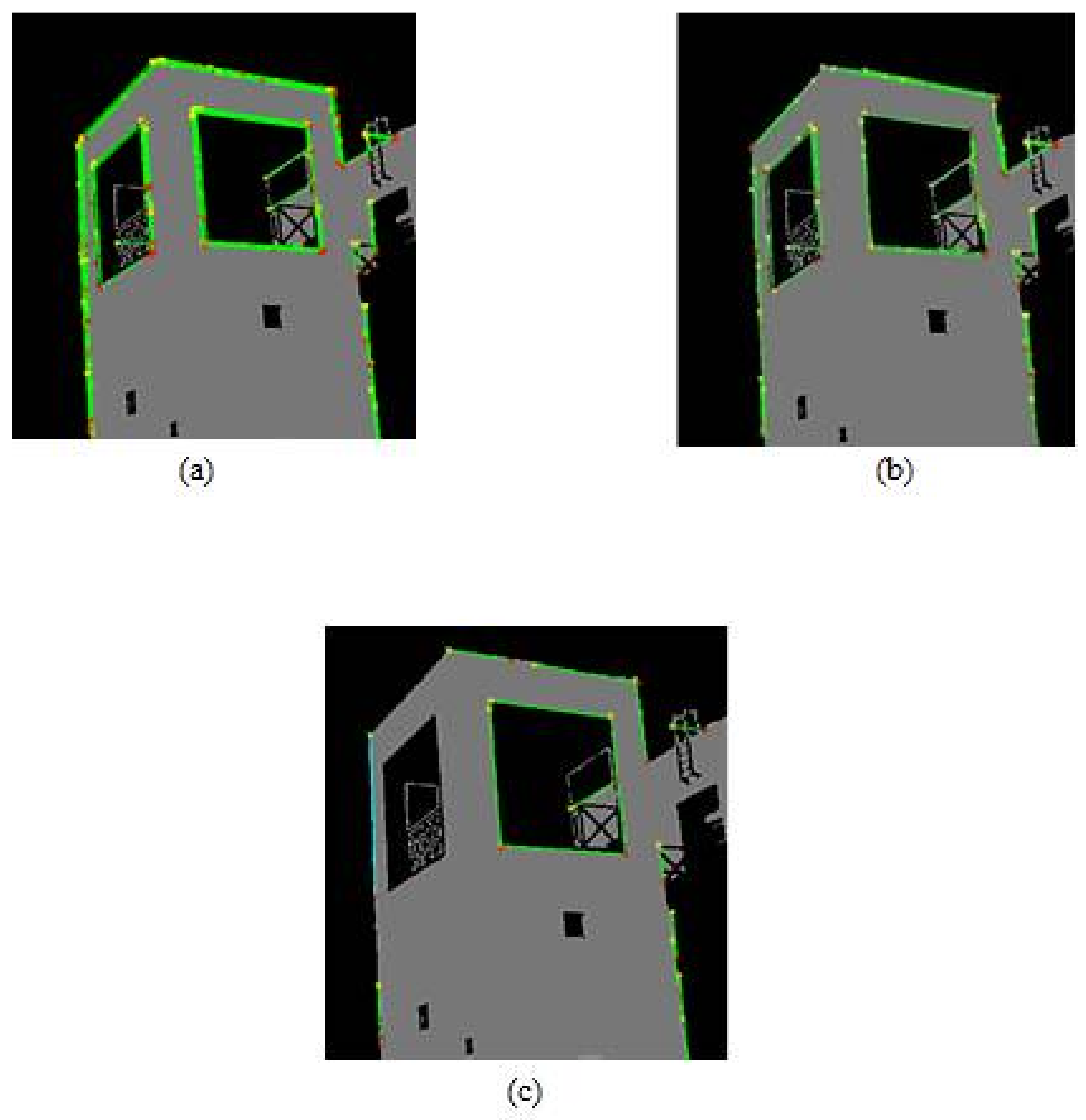
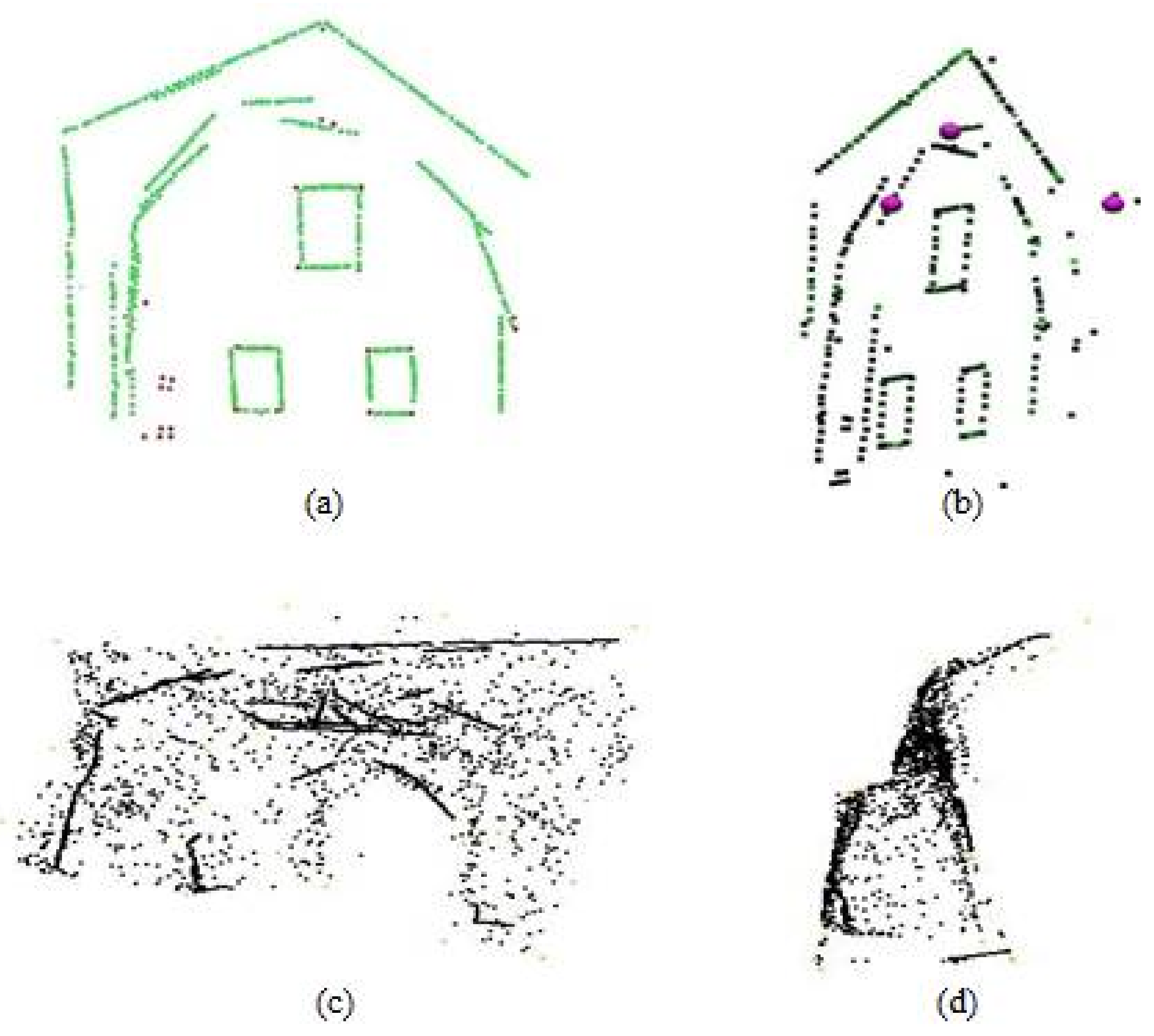
Furthermore, in cases of high structural information, the sequential application of edge and line extraction processes will produce multiple “strong” line segments describing the same region, as illustrated in
Figure 4a. Our solution to these problems, presented in detail in [
31], was the formulation of a line segment strength evaluation scheme that selects the strongest line segment. This is achieved through a weighting function that ranks the line segments considering positional relations and length characteristics. Specifically, for each line “
j”, its strength/rank is determined by the following function:
where
N corresponds to the amount of line segments estimated in the interrogation window, which is located at the Hough position of the examined line
j,
DistStart and
DistFin correspond to the Euclidean distances of the starting and finishing points of the line segments and, finally,
len corresponds to the length of the examined line
j. The weights, w, denote the importance of each parameter on the overall result. All weights sum to 1, with the first weight having the largest value, since the starting point of each line segment plays an important role in the formulation of the interrogation window of the examined line. This ranking scheme allows us to remove redundant line segments, which describe the same region. In order to further strengthen the line-based representation, we introduce in this paper two additional conditions that lead to (a) the merge of collinear line segments resulting in a better description of the region and, (b) to the appropriate selection of parallel line segments.
Line Segment Co-Linearity Condition: Given an examined line defined by its starting point
and its ending point
and
the starting point of a neighboring line segment define the distance
as:
In the case of co-linear line segments, the distance is zero. When such a condition is fulfilled these line segments are merged producing a single line segment that has the longest possible length (based on the starting and ending points of the two co-linear segments).
These two constraints are in accordance with the line strength evaluation and selection criterion, which lead to the derivation of an accurate line-based description of the building’s 2D structural skeleton.
Figure 4 depicts the accuracy increase in the case of the campus building façade due to the application of the sequential edge—line segment—line strength evaluation scheme, as well as the addition of the two Skeleton refinement conditions. We can observe a significant decrease of the overlaid line-segments on each region (indicated by red and yellow dots). However, the performance of this process depends on the size of the examined region, an effect that can be observed in
Figure 4b,c. In our approach we have selected a block size of 17 × 17 pixels.
2.3.3. Inner Feature Extraction and Description
The next stage of the skeleton extraction process is the identification of the inner building façade structures, such as windows or doors. The stereoscopic-driven depth map allows the estimation of the protrusion of these inner features [
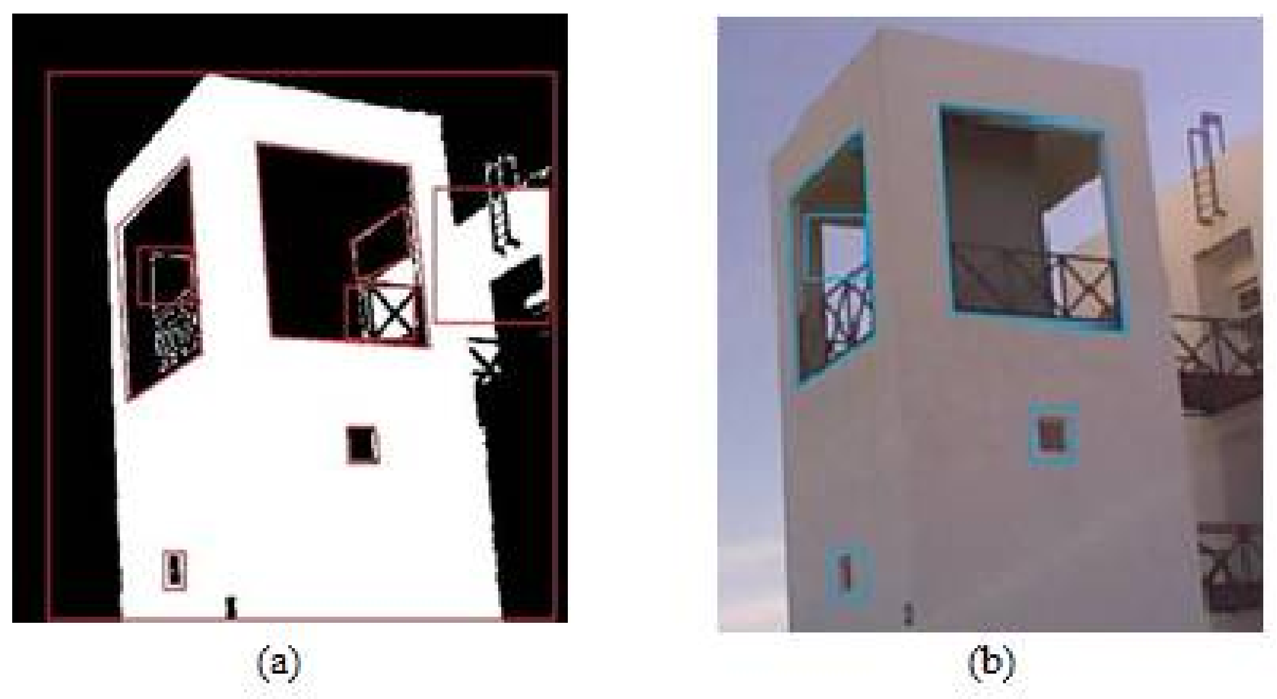
31]. This process involves the detection and description of these features and the relation of these features with their corresponding depth information. We take advantage of the shape characteristics of the structures. Under the assumption of rectangular-shaped structures, we initially identify candidate object regions in the derived building contour and then a rectangle fitting methodology is applied based on the shape properties of each region. In order to exclude erroneous detections we introduce a threshold-based scheme that considers the amount of non-zero points contained in the identified region. A low number of non-zero points (threshold set experimentally to 30%) indicates a successful identification. Moreover, an additional constraint regarding the windows was included which is based on the size of the rectangle, indicating candidate window regions, and the dimensions of the image. Candidate rectangles that are larger than the ¼ of the image’s size (total number of pixels) are suppressed, since it is unlikely to correspond to a feasible window.
Figure 5 illustrates the application of the proposed inner façade structure detection approach on the campus building. As can be seen in
Figure 5a prior to the application of the threshold, we end up with erroneous identifications, which are eliminated when the pixel value condition is applied (blue marked rectangular regions).
Another source of erroneous detections, as well as non-detection cases, is the perspective projection that is introduced during the image acquisition process. Projecting into a lower dimension introduces deformations on both the shape and the size of the structure. The severity of these deformations depends upon the camera’s position, orientation, and field of view. This means that rectangular windows may not appear rectangular at all. To overcome such projection-related problems we exploit additional information about the acquisition layout and monitoring process (interior and exterior parameters) and correct the deformations (by removing lens distortion). Alternatively, we can take advantage of some additional knowledge about the dimensions of the structure acquired from other sources, such as geodetic measurements. The additional information provides the necessary data to correct the deformations via orthorectification [
34]. In our test cases the camera layout faces the structure leading to minimum deformation on the shape of the inner structures (e.g., windows) and, thus, the detection is not largely affected by the projection as shown in
Figure 5. Moreover, as we mentioned in the previous section, a stage without distortion precedes the morphological operations (i.e., segmentation, skeleton extraction). Future work will focus on resolving projection-related structure shape deformations due to extreme viewing angles that can undermine the detection accuracy.
2.4. Georeference, Depth, and Building Skeleton Relation
Relying only on image-based data for 3D reconstruction requires specific monitoring constraints, here meaning front-facing viewing images, parallel (non-convergent) camera layout and careful planning that will minimize the reprojection errors and reconstruction uncertainty. Even then, the data do not suffice for accurate 3D model reconstructions. The majority of existing methods enrich these sparse 3D point clouds with auxiliary data from other sources, such as laser scanning devices or geodetic stations. In our approach we combine image data with georeferenced data acquired using tacheometry. A total station was employed for the digital recording of the surveyed points. The data consist of three dimensional coordinates
x,
y,
z, or easting, northing, and elevation, which are computed taking as input the initial on site measurements using trigonometry and triangulation. A distance accuracy of ±2 mm to ±5 mm was inherent for each point (total station error). The surveying of the Neoria building was also used in previous work [
41]. The final obtained raw data are in the form of Greek Geodetic Reference System 87 (GGRS87) coordinates. The GGRS87 is a geodetic system commonly used in Greece. The system specifies a local geodetic datum and a projection system [
42].
In order to combine the two information sources (image and geodetic datasets) we define a mapping scheme that relates the 2D image point coordinates and the 3D coordinates of the georeferenced dataset. The mapping initially involves the creation of a fictitious 3D space xim-f, in which the 2D coordinates are augmented and interpolated into a 3D coordinate space using a variable z0 as a fixed third dimension. By a manual or feature-based selection of point correspondences between 2D image points and its georeferenced coordinates, we can define a mapping transformation function that provides the relation between the 2D image plane coordinates (the 2D building skeleton) and the 3D georeferenced point dataset. More details will be presented in the following sections.
The last step of our 3D model reconstruction framework involves the extraction of information concerning the structural details of the structure’s façade thus assisting the refinement of the resulting 3D object.
2.5. Image-Based Depth Information
The georeferenced data contain information about general dimensions and position of the structure. Thus, we can only recover a crude 3D reconstruction of the basic shape of the structure. In order to further refine the 3D model, we can utilize additional information that can be extracted from an image-driven depth map.
In our approach we utilize a calibrated stereoscopic layout, with known interior and exterior layout parameters, to extract the depth map of the scene, using the method of triangulation [
34]. From this depth map we then extract depth-related information about the inner façade structures of the building, such as windows or doors, which, in our case, is their protrusion information. This task requires us to associate the depth information with the inner façade structures. In order to achieve that we first detect those inner structures in the image plane domain, by applying a rectangle fitting methodology, based on each image region properties, and then associate the corresponding pixels with their depth information. Finally, as presented in our previous work, we can compute the protrusion, of the rectangular inner structure (e.g., door, window or ledge), by simply computing the difference of the average depth of the pixels belonging to inner structure and the pixels belonging in the foreground wall region that surrounds this inner structure.
4. Results
4.1. Test Cases
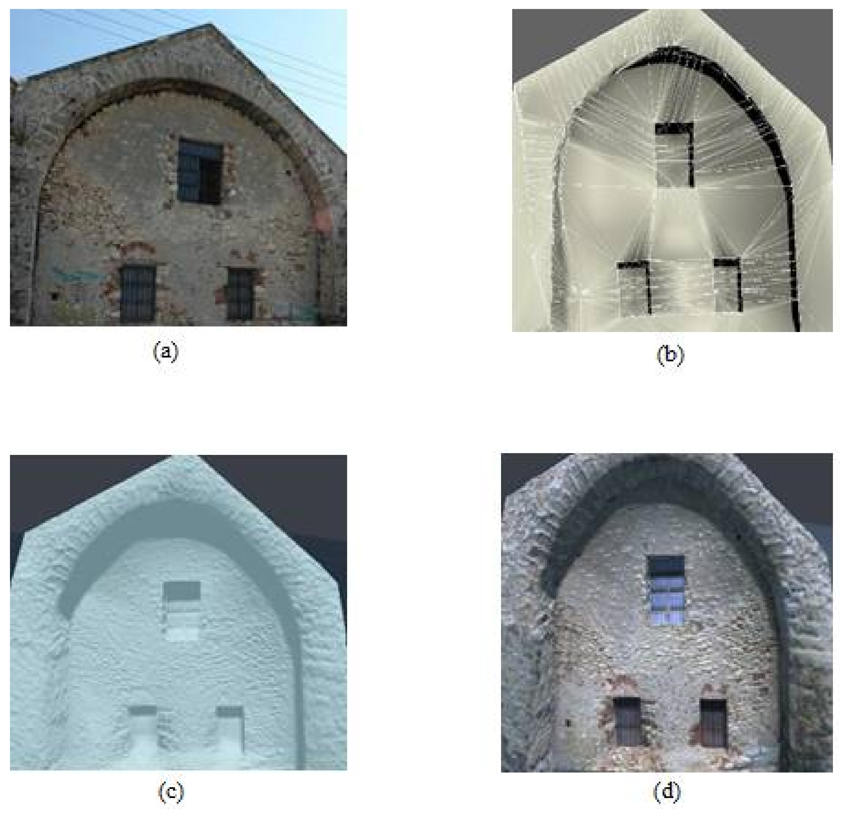
We will now examine the results of each stage, further commenting on the implementation issues and reconstruction accuracy. The initial stage of the method involves the registration of the 2D skeleton of the building with the georeferenced point dataset, producing an initial 3D point cloud.
Figure 6 depicts the 2D skeleton of the Neoria building front façade (
Figure 6a,b), as well as the right side façade (
Figure 6c,d).
The registration of the georeferenced data using the Equation (4) and the employment of the interpolant expressed in Equation (6) recalculates the third coordinate (z
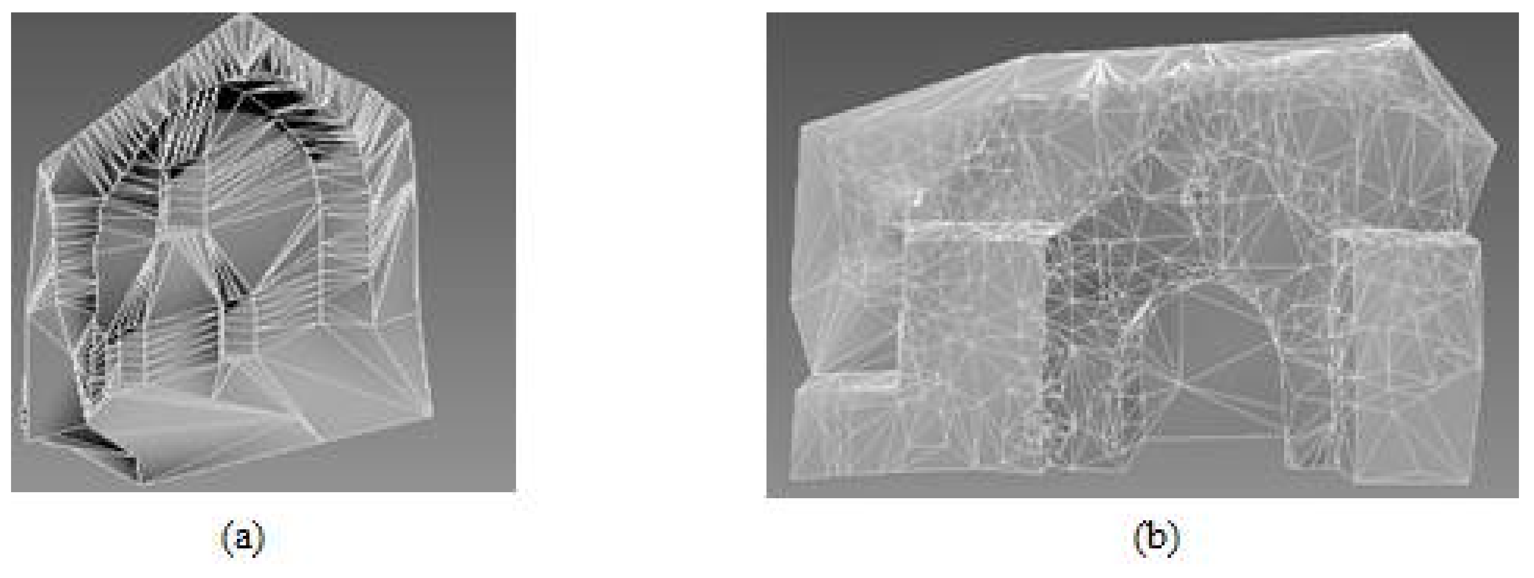
0) to add the depth information. Therefore, the skeleton point cloud is enriched with the depth attribute. Then, Delaunay triangulation [
40] constructs an initial mesh based on the augmented point set as shown in
Figure 7 for the Neoria front and right façades. Stereo image data specify the structural basis of the façade (by providing the original skeleton) and, thus, refinement of the 3D model is achieved with a limited amount of georeferenced data.
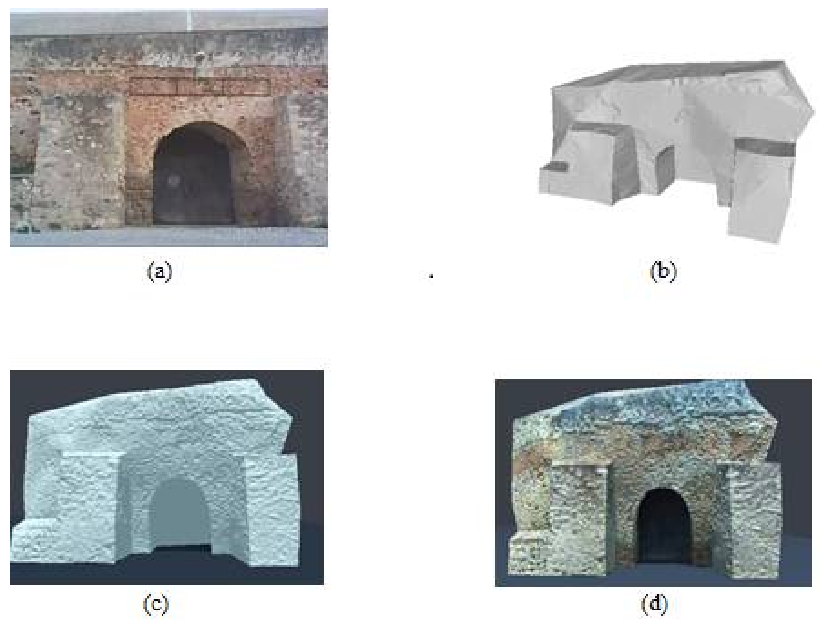
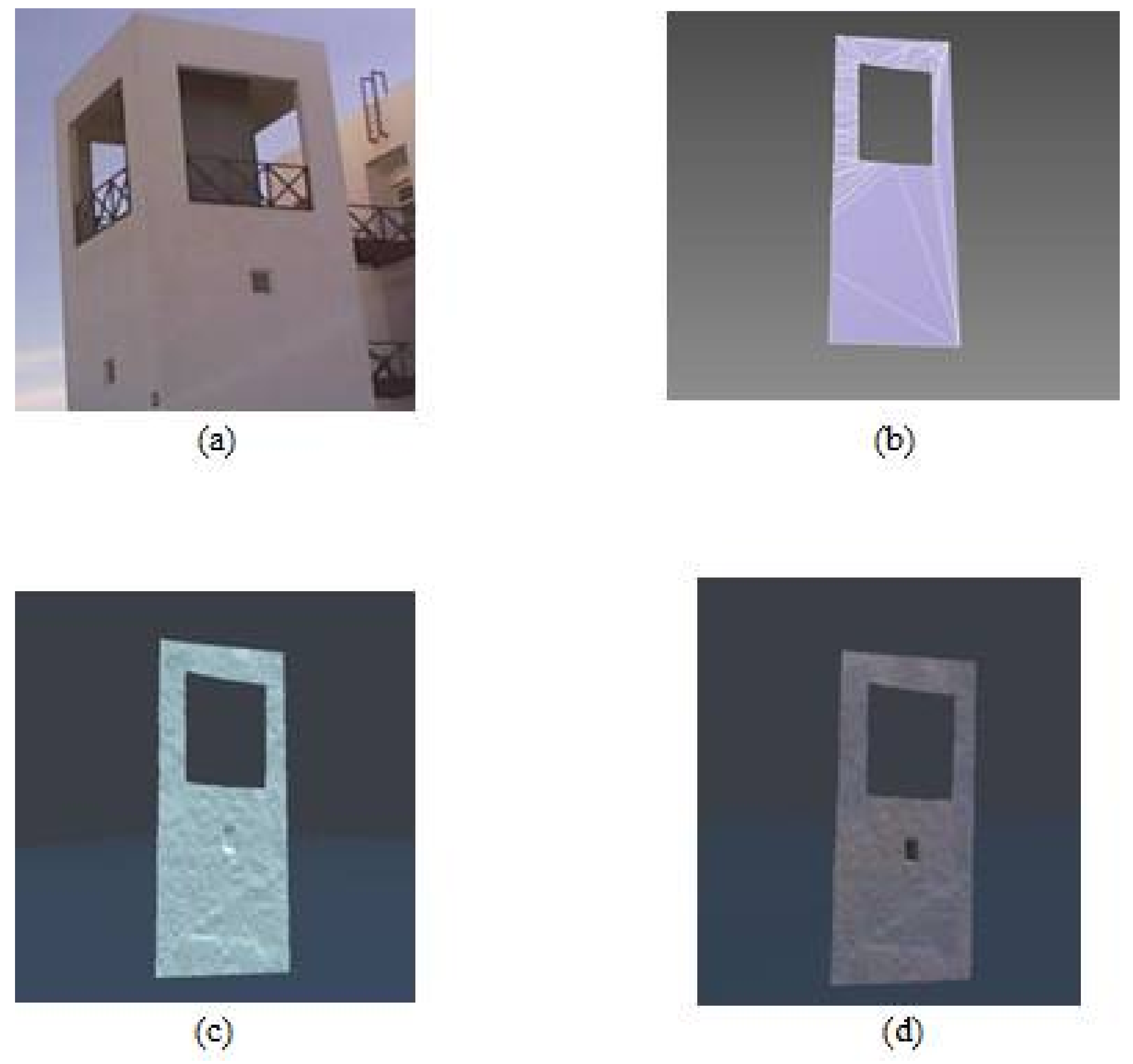
The following step involves the refinement of the inner building feature details with protrusion addition for the windows, doors or ledges, as it has been estimated based on the stereo-driven depth map. In the final stage of the reconstruction process, the realistic fidelity of the model was enhanced by texture mapping and illumination effects. The texture addition, i.e., the surface’s main color, was implemented by a process called diffuse mapping which wraps image samples onto the surface and displays the pixel color. The procedure involves the assignment of image pixels in particular surface places and was implemented via Autodesk 3ds Max software (Autodesk Inc). Additionally, the model was imported into the Unity 3D graphic software, which provides the tools to implement illumination and shading techniques. The realism of the scene was particularly increased by normal mapping, a photorealistic technique) that simulates the lighting process by taking the dot product between the unit vector of the model’s surface and the unit vector of a simulated light source.
Figure 8,
Figure 9 and
Figure 10 depict the 3D model achieved using the aforementioned process, for the test cases of the Neoria building front and right face façades, as well as the campus building.
The depth information generated by the stereoscopic layout is only used for the protrusion estimation process of the inner features of the building. This is due to the fact that the reprojection distortions are more severe in the outer skeleton of the building and increase exponentially as the monitoring range and building size increases. To reduce the reconstruction distortions and reprojection errors we can potentially exploit auxiliary information about the scene/structure and impose additional scene constraints, such as 3D line parallelism, as well as utilize prior hypotheses about the structural characteristics of the entire building or for specific parts (e.g., trying to find a skeleton that fits a specific set of shape patterns, for example, a rectangle, or a triangle (when rooftops are present)).
The case of the campus building presents difficulties related to the topography of the area, which does not allow for clear front-facing viewing positions, and the height of the building. Non-facing viewing angles introduce projective deformations due to perspective effects. The eventual deformations, although not severe, are passed on to the 3D reconstruction process. Less depth information can be extracted, since the larger and taller structure augments the viewing distance. As the viewing distance grows the projective ambiguities and errors increase, leading to erroneous depth estimates.
In such viewing cases, we only rely on the extracted 2D structural skeleton of the building the interpolation accuracy between the 2D image data and the georeferenced data based on specific key points that have been detected. This interpolation suffices to extract the depth attribute of structure (reconstruction of the inner façade structures cannot be performed since we lack the stereoscopic depth driven protrusion information). Additionally, the obscure viewing angle for the specific viewing case (
Figure 10a) leads to the elimination of two façade walls in the images. Taking this into consideration, along with the purpose of illustrating the skeleton extraction process in the first stage of our approach, the features of both façades (walls) were detected. However, the georeferenced based interpolation surface that is employed during the reconstruction process is characterized by a consistent orientation, which means that it can be utilized for a single-sided structure (façade). This condition results in only one wall of the structure being adequately reconstructed. A correction of the perspective distortion in the future will further extend the variety of cases covered with our approach.
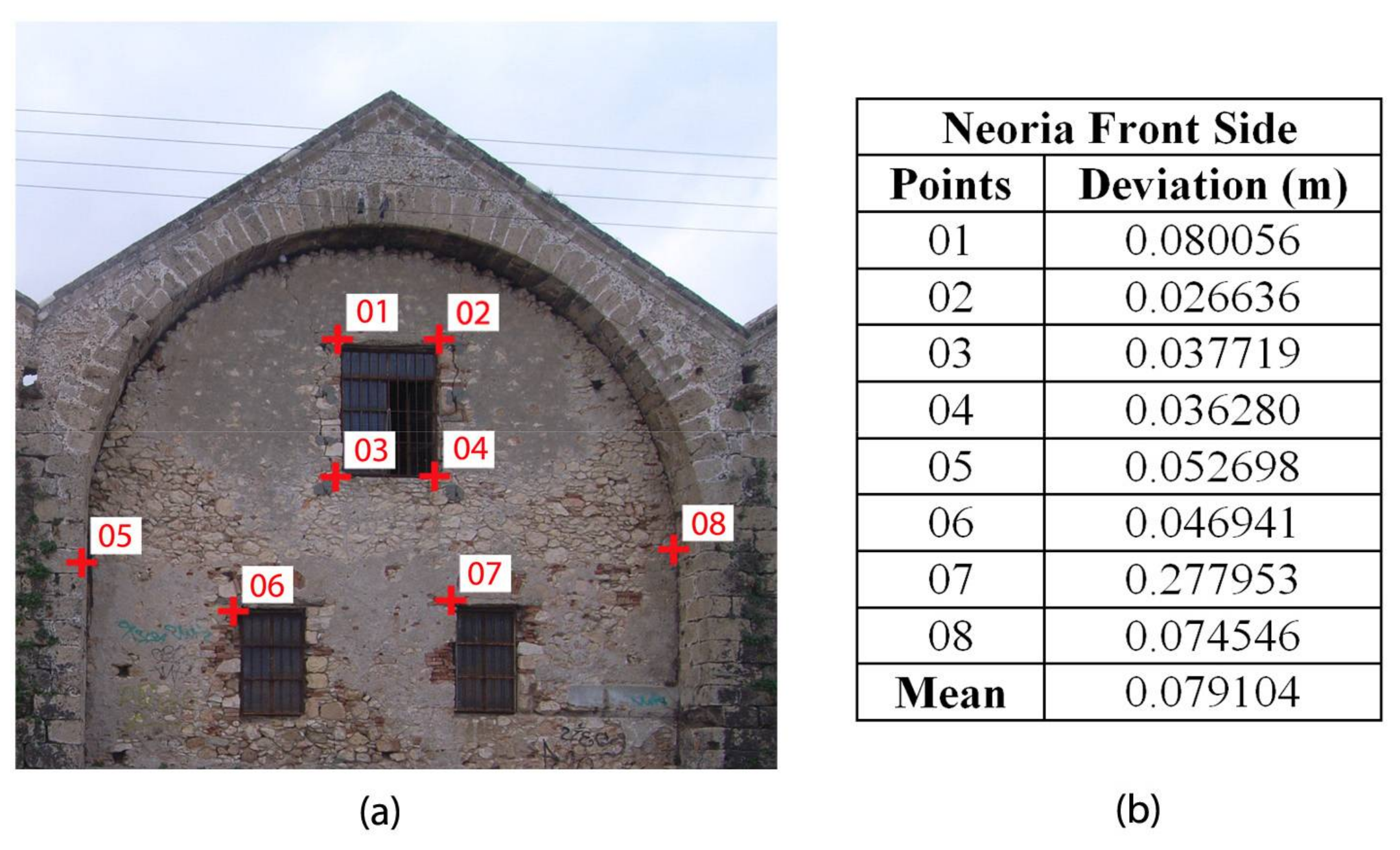
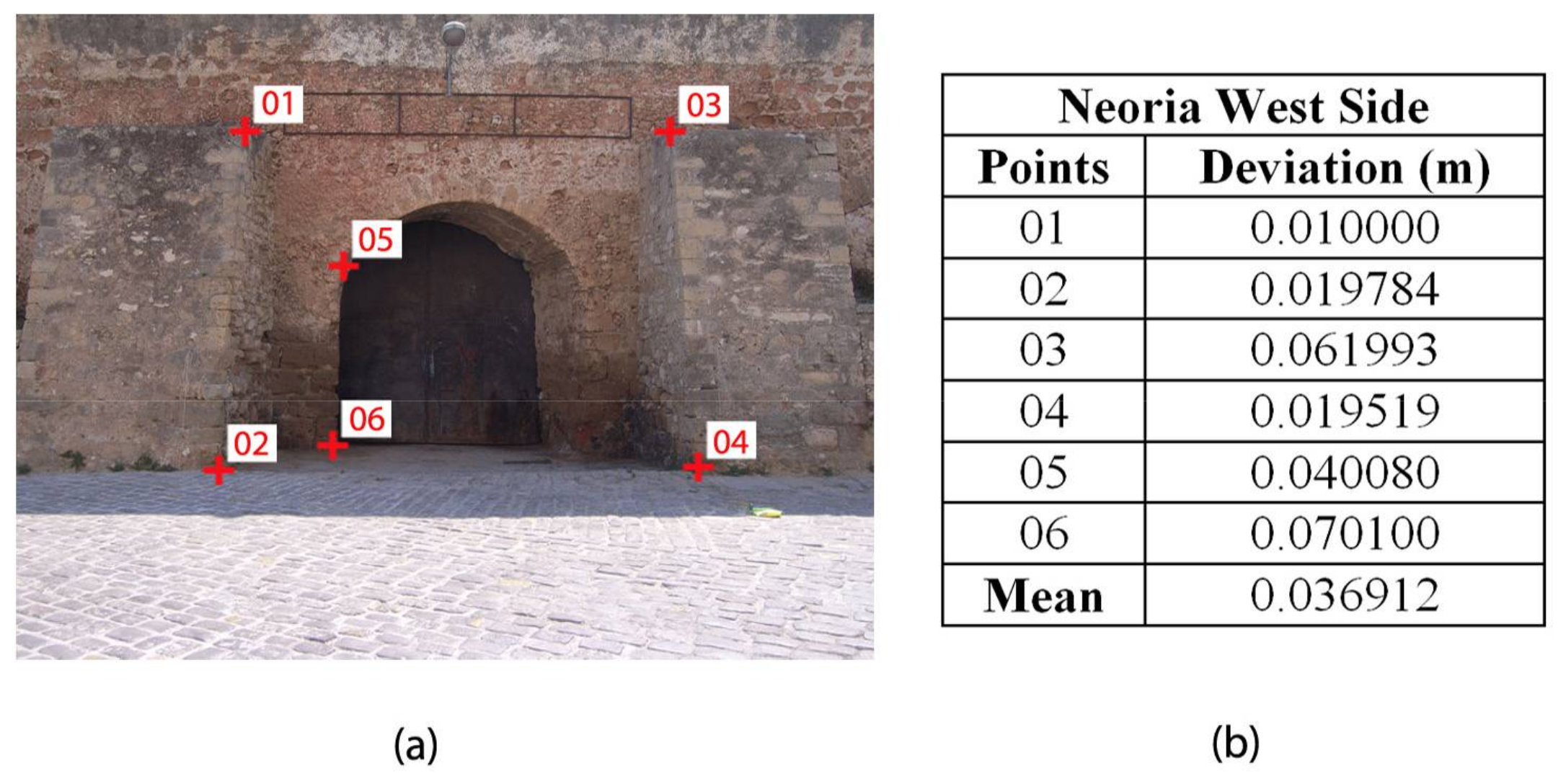
4.2. Quality Evaluation of the 3D Model
In order to validate the methodology, proper quality assessment is necessary [
44]. The results along with the effectiveness of the proposed method for each façade are evaluated in two stages. First, an accuracy assessment is carried out through the employment of ground control points. Secondly, a geometric evaluation of the final façade 3D object is implemented in order to quantify the effects of the methodology on the data. A quantitative analysis of the accuracy of the results requires an independent reference dataset. To that end, ground control points (GCP) were appointed across the façades in easily identifiable areas. GCP-based analysis and evaluation of the resulting 3D model quantifies the effect of the methodology on the quality of the final result [
45,
46]. In our study, GCP were measured using a total station and expressed in GGRS87 for consistency. The distribution of the GCP in each façade is shown in
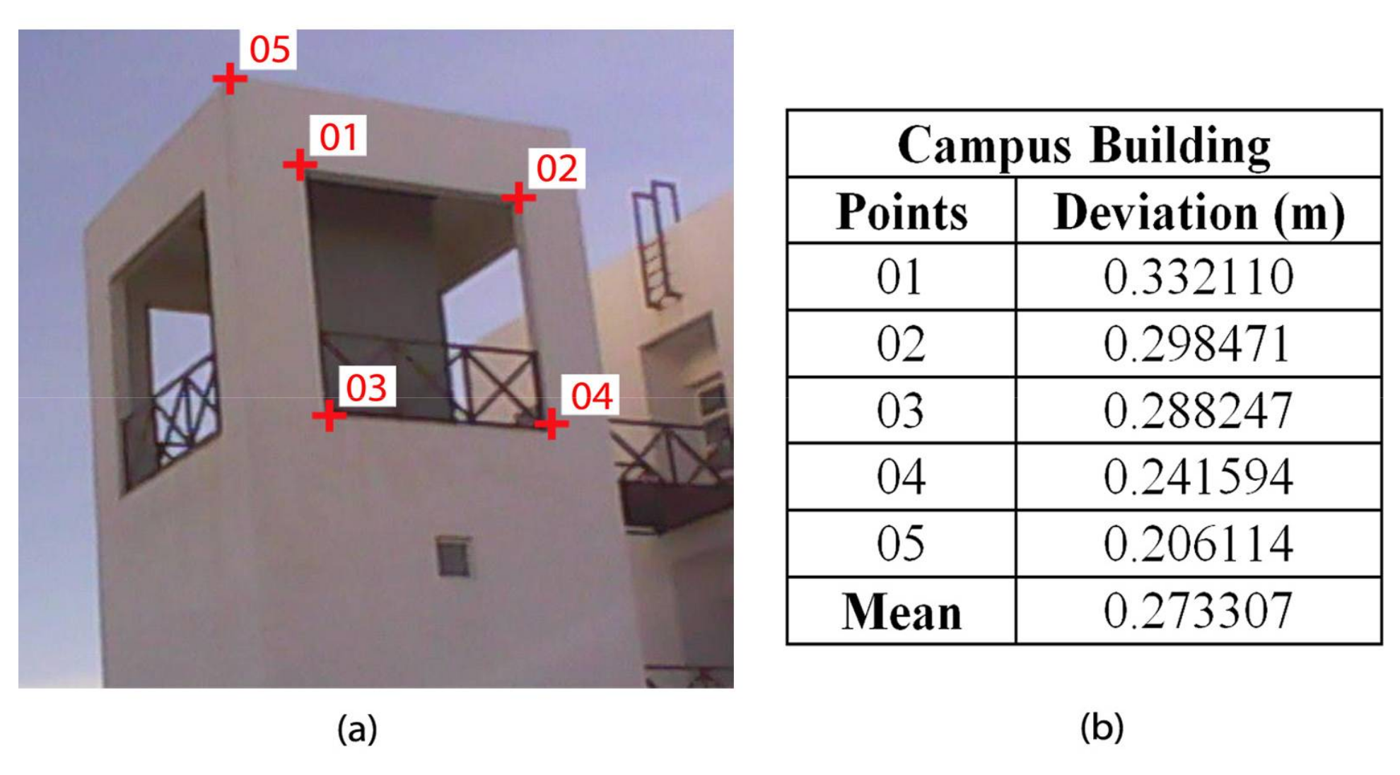
Figure 11a,
Figure 12a, and
Figure 13a. The distribution of the GCP was even on the façade
Figure 11a and
Figure 12a. However, in
Figure 13a we had GCP only at the upper part of the building.
The GCP were manually selected amongst the vertices of the final 3D model of each façade and their measured coordinates were compared to the known GCP coordinates from the tacheometric survey. The known GCP coordinates were employed as independent reference. The assessment focuses on the computation of the 3D deviation between corresponding point pairs in the two data sets. The spatial deviations of each GCP are presented analytically in
Figure 11b,
Figure 12b, and
Figure 13b. The mean 3D deviation for each façade was also computed. The discrepancy between the Neoria façades and the campus building façades is to be expected. A mean deviation of about 27 cm on the campus building was calculated. That discrepancy is generated by the displacement of the final surface points, a consequence of the initial image perspective distortion. The Neoria façade models are more accurate. The mean deviation of the front side façade is estimated at ~8 cm, while the west side façade has achieved a mean deviation of ~3.7 cm. The quantity of the initial GCP data used in the reconstruction process is considered a factor for that differentiation, as the amount of georeferenced data fused in the point cloud representing the skeleton of the west side was higher than those used for the front side.
Additionally, errors could appear through the workflow, potentially affecting the reliability of the 3D model. The procedure of the surface creation, the exchange between software, and the post-processing of the 3D model can affect the quality of the final result. In regard to that, a geometric evaluation is carried out based on tacheometry measurements of the same type used in the methodology and acquired with the same total station. Although there is a possibility of the newly-acquired raw data being almost identical to the first measurements, we consider them a sufficient means to provide an assessment regarding the quality of the reconstruction. If anything, we can gain an interesting insight with respect to the relation of the input data and the output 3D model.
The goal of this evaluation method is to determine whether the positioning of points in the resulting 3D reconstruction has deviated from the geographic raw data originally measured on site. In this manner, an error calculation can be relevant to the georeferencing of the building reconstruction.
In this case the geometric evaluation of the model is analyzed by computing its deviation from the geometric raw data. A ‘nearest neighbor distance’ method was applied. The raw data measurements were considered the reference entity. The essence of this method is that for each point of the 3D model’s triangular mesh, the nearest point in the reference data is located and their Euclidean distance was computed. The process was executed in CloudCompare (GPL software). The point deviations are depicted on the model by a scalar field color scale. They are in absolute distances and in meters. The respective histogram portrays the distribution of the points according to their deviation from the reference data.
Analyzing the deviation of surface points of the west side part, as shown in
Figure 14a, the predominant set is the one with a distance difference less than 10 cm from the reference data. The green surface areas with medium deviation ranging from 40 cm to around 1 m represent the parts not containing raw reference data information nearby. This issue is most notable at the inwardly-protruded door surface (red color), providing the largest deviation due to the complete lack of that section’s geographic information. Regarding the front side part of Neoria (
Figure 14c), the key façade features have minimum deviation, around 10 cm. In this case the raw data were sparse and pertaining to the points of interest, leading to the occurrence of higher deviations in regions with an absence of them.
The evaluation of the campus building case (
Figure 15a) is expected to include deviations due to the geometry deformations caused by the initial projection distortion. The major deformations are detected around the window, whose rectangular shape makes the distortion more apparent.
5. Conclusions and Future Work
This paper presents an extension on our previous work [
31] tackling the problem of fusing multimodal sensor data for constructing a 3D model of a structure/building. The proposed methodology requires low-cost data acquisition equipment, mainly, an image acquisition device and a georeferenced dataset obtained with the use of a total station. The combination of imaging datasets and image-driven depth maps with the georeferenced point dataset allows the accurate reconstruction for the structures. The main point of the paper is that even with highly available and inexpensive equipment we can produce 3D models of structures, emphasizing in this paper the building façade reconstruction accuracy, provided that we use sophisticated data processing techniques and multimodal data sources.
Concerning the image dataset specifications, both stereoscopic and single camera images are used, acquired through a setup of CCD cameras. The stereo setup and the produced depth map has limitations due to reprojection errors that restrict the contribution of GCP data in the final model.
The presented approach is subject to improvement concerning the amount of information that can be derived from the image and image-based depth map dataset. By reducing the reprojection distortions and introducing scene and structural constraints and assumptions, we hope to enrich the depth-map accuracy and increase its contribution to the reconstruction process. The goal is to eventually use the image-based depth point cloud as a first crude 3D model basis, rather than the extraction of the protrusion estimates, with the additional gain of further reducing the amount of georeferenced data points used in the reconstruction process.

 ,
, 


