An Object-Based Image Analysis Workflow for Monitoring Shallow-Water Aquatic Vegetation in Multispectral Drone Imagery

Abstract

High-resolution drone aerial surveys combined with object-based image analysis are transforming our capacity to monitor and manage aquatic vegetation in an era of invasive species. To better exploit the potential of these technologies, there is a need to develop more efficient and accessible analysis workflows and focus more efforts on the distinct challenge of mapping submerged vegetation. We present a straightforward workflow developed to monitor emergent and submerged invasive water soldier (Stratiotes aloides) in shallow waters of the Trent-Severn Waterway in Ontario, Canada. The main elements of the workflow are: (1) collection of radiometrically calibrated multispectral imagery including a near-infrared band; (2) multistage segmentation of the imagery involving an initial separation of above-water from submerged features; and (3) automated classification of features with a supervised machine-learning classifier. The approach yielded excellent classification accuracy for emergent features (overall accuracy = 92%; kappa = 88%; water soldier producer’s accuracy = 92%; user’s accuracy = 91%) and good accuracy for submerged features (overall accuracy = 84%; kappa = 75%; water soldier producer’s accuracy = 71%; user’s accuracy = 84%). The workflow employs off-the-shelf graphical software tools requiring no programming or coding, and could therefore be used by anyone with basic GIS and image analysis skills for a potentially wide variety of aquatic vegetation monitoring operations.

1. Introduction

A third of the world’s worst aquatic invasive species are directly linked to the aquarium and ornamental industry [1]. Once these species are introduced into natural waterways, they extensively modify the biological communities and disrupt many of the important ecological and cultural services that we have come to depend upon from our freshwater inland ecosystems. They also cause significant economic impacts, both in terms of the costs associated with management/eradication, as well as the overall “devaluation” that is associated with presence of the invader. Rockwell [2] estimated that over US$100 million is being spent annually in the United States to control and manage invasive aquatic plants.

Water soldier (Stratiotes aloides) (Figure 1) is a perennial aquatic plant species native to Europe and northwest Asia that was introduced into the Trent-Severn Waterway in Ontario, Canada, likely as a result of its popularity as an ornamental plant in water gardens before being banned [3]. It grows most effectively at water depths up to 2.5 m, but has been found at depths up to 5 m. It becomes buoyant during the summer season, with plants reaching above or near the surface where it can form dense mats that crowd out native vegetation, alter water chemistry, and consequently modify phytoplankton populations and potentially other aquatic organisms. Its sharp serrated leaves can injure swimmers, and generally the plant hinders various other aquatic activities, such as boating and angling [3]. Because the Trent-Severn Waterway is the only place in North America where water soldier is known to occur, it is considered a high priority to prevent it from spreading to new locations, notably the nearby Great Lakes. Since water soldier was discovered in the waterway, resource managers and their partners have been trying to eradicate the plant through repeated large-scale applications of chemical herbicide (diquat), but have been met with mixed results as the plant continues to show up farther downstream.

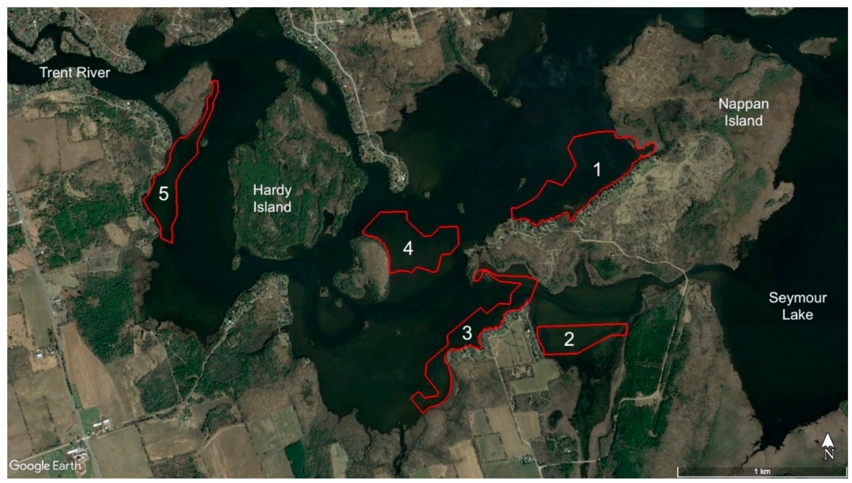
Current boat-based detection and monitoring methods in the area of infestation and locations downstream include both systematic (whole lake surveys) and opportunistic monitoring (incidental spotting); however, the type of data collected, although helpful, can be limited and unreliable [4]. In particular, the point-based sampling method provides incomplete coverage of surveyed areas, and deeper (>1 m) submerged vegetation can sometimes be difficult to detect. Due to the nature of the Trent-Severn Waterway, many sampling sites are inaccessible, as they are too shallow, blocked by obstacles, or in remote regions, making boat-based monitoring time-consuming and expensive [5].

In recent years, there has been burgeoning use of small drone aircraft systems to conveniently collect timely, very high spatial-resolution (<20 cm) imagery of hard-to-access or -navigate aquatic environments, including wetlands [6,7,8], bogs [9,10,11], lakes [12,13,14], rivers [15,16,17], coasts [18,19,20], and general hydrological and water resource monitoring [21,22,23]. As high-resolution drone imagery tends to be laborious to analyze manually, increasingly sophisticated approaches have been developed and tested to automate such tasks as aquatic vegetation detection and classification, many of them founded on object-based image analysis (OBIA) [24,25,26,27,28]. However, few studies have involved the distinct challenge of automated classification of submerged vegetation [29,30,31]. Moreover, although drones themselves are becoming increasingly accessible and easy to use, there is a need to establish more accessible workflows for efficiently analyzing the imagery they generate.

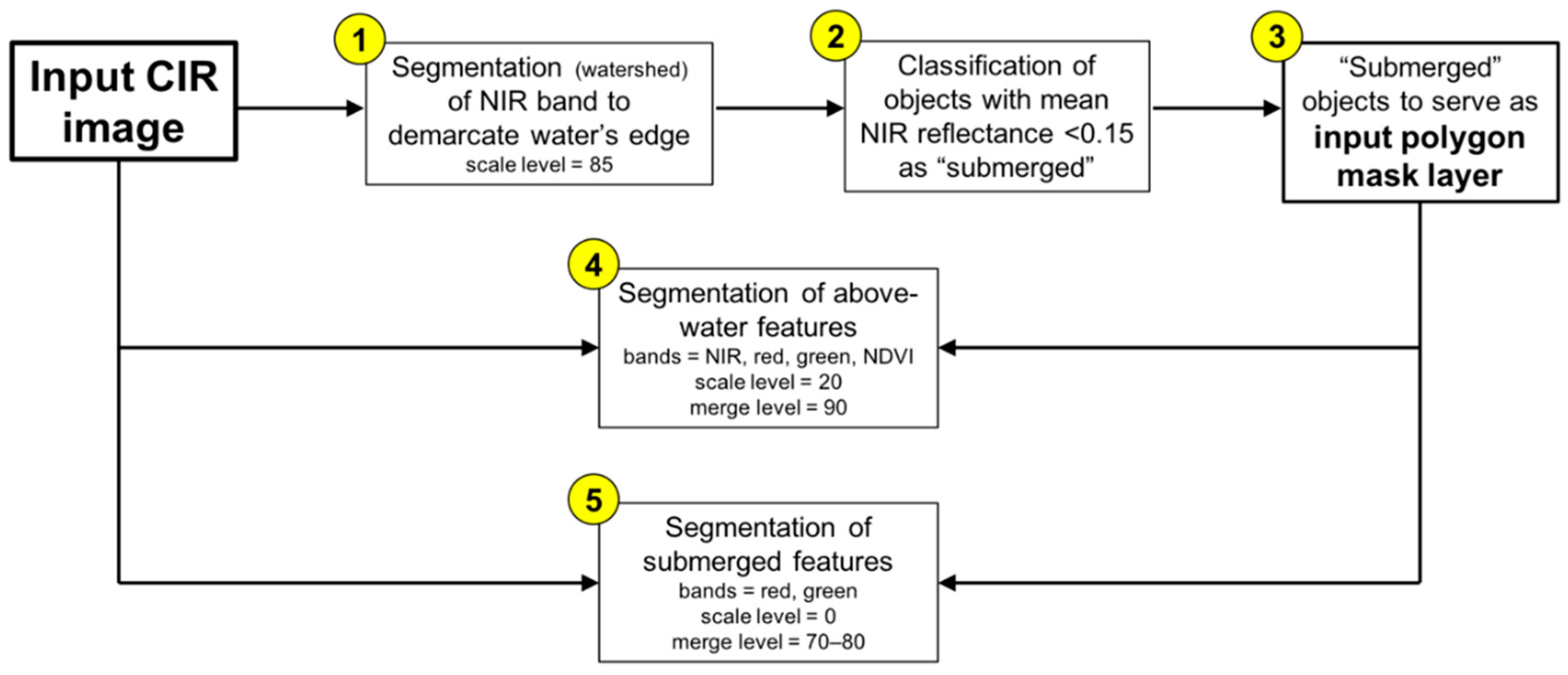
Building upon a previous pilot trial [32], our aim was to develop an efficient and readily accessible drone imagery acquisition and OBIA workflow for monitoring emergent and submerged water soldier. In this paper, we present and assess our workflow, which we believe could be broadly adapted to other shallow-water aquatic vegetation monitoring operations. The principal elements of the workflow are: (1) collection of radiometrically calibrated multispectral imagery, including a near-infrared (NIR) band; (2) multistage segmentation of the imagery involving an initial separation of above-water from submerged features; and (3) automated classification of image features by means of a supervised machine-learning classifier.

2. Materials and Methods

2.1. Study Area

This study focused on the region of the Trent-Severn Waterway known as Seymour Lake (Figure 2), which is considered to be ground zero of the water soldier infestation. Five discrete study sites totaling ≈60 ha were selected for drone aerial surveys, each representing a previously established experimental water soldier treatment site. They are largely dominated by water soldier, where total plant biomass can approach levels up to 8000 g·m⁻² (wet weight). Water depths in all sites range between 0.5–2.0 m, and other co-occurring aquatic plant species include Vallisneria americana, Myriophyllum spicatum, Elodea canadensis, Ceratophyllum demersum, Potamogeton zosteriformis, Nymphaea odorata, Nuphar variegata, Brasenia schreberi, Pontederia cordata, and Typha spp. The cumulative biomass of these other species is typically 300–500 g·m⁻² (wet weight). A field survey of the study sites was conducted during August 2016 as part of a separate project. A 33 × 33 m grid of sampling points covering each site was created in a geographic information system (GIS), and the points were navigated to in the field using a handheld global position system (GPS) receiver. At each point, the dominant vegetation (if any) was recorded, providing a coarse dataset to aid in the interpretation of fine-resolution aerial imagery.

2.2. Data Collection and Post-Processing

We collected aerial imagery over the five study sites on 14 October 2016—by which time water soldier colonies had fully expanded—between 10:00 and 16:00 local time, under mostly overcast sky conditions with minimal wind. We used an eBee mapping drone (senseFly, Cheseaux-sur-Lausanne, Switzerland) carrying a Sequoia multispectral camera (Parrot, Paris, France) that captures 40 nm wide bands centered in the green (550 nm), red (660 nm), and NIR (790 nm) regions, a 10 nm wide band in the red-edge (735 nm) region, as well as supplementary standard true-color (RGB) imagery through a dedicated sensor. Although we recognized from the outset that a multispectral camera with a blue band would likely yield superior detection of submerged vegetation, we did not have access to such a sensor at the time of the study and decided to use the Sequoia, which was available as a pre-existing resource. The drone was flown at an altitude of 400 ft (122 m) above ground level, yielding a spatial resolution of ≈13 cm for the multispectral imagery and ≈4 cm for the RGB imagery. Images were captured with 80% forward overlap and 70% lateral overlap.

We performed photogrammetric post-processing of the imagery with Pix4Dmapper Pro 3.0 (Pix4D, Lausanne, Switzerland). We created a basic RGB orthomosaic (Figure 3A) of each of the five study sites for the purpose of assisting with visual interpretation of the multispectral imagery. The multispectral imagery was radiometrically calibrated using a combination of data recorded concurrently with image capture by the Sequoia’s downwelling light sensor mounted on top of the drone, as well as a spectralon calibration panel (AIRINOV, Paris, France) photographed on the ground prior to each flight. The images were then mosaicked and rendered into absolute reflectance maps (pixel values ranging from 0–1) for each of the spectral bands. Using QGIS 2.18 (QGIS Development Team), we created three-band false-color (i.e., color-infrared; CIR) composite images of the study sites by merging the NIR, red, and green reflectance maps (Figure 3B), then merged the images of the five sites into a single raster file. Finally, we clipped out portions of the imagery extending beyond the boundaries of the study sites, leaving only areas containing water and aquatic vegetation of interest and excluding extraneous features, such as terrestrial vegetation and man-made structures.

2.3. Image Segmentation

We performed image segmentation with the Feature Extraction module in ENVI 5.4 (Exelis Visual Information Solutions, Boulder, CO, USA), which employs a “watershed” segmentation algorithm [33] and allows quick testing of segmentation parameters by previewing results in a small window that can be panned over the input image prior to fully executing segmentation. Following segmentation, a set of classification attributes is calculated for every resulting object—including 14 spatial attributes (variously describing object size, dimensions, and shape), four spectral attributes per band (minimum, maximum, mean, and standard deviation), and four first-order texture attributes per band (mean, range, variance, and entropy within a texture kernel of adjustable size [34])—and recorded in an attribute table accompanying the outputted polygon shapefile containing the objects. The multistage image segmentation approach we employed is summarized in Figure 4 and detailed below.

2.3.1. Separation of Above-Water and Submerged Features

Because submerged features have a significantly muted and less contrasting appearance in imagery compared to above-water features, wholesale segmentation of imagery containing both above-water and submerged features of interest tends to entail an unworkable trade-off between over-segmentation of the former (features are subdivided into numerous small objects) and under-segmentation of the latter (features are lumped into larger objects containing other adjacent or encapsulating features) [32]. To circumvent this issue, we exploited the extremely high absorption of NIR radiation in water, resulting in submerged areas having a nearly to completely black appearance in the NIR band. We performed an initial segmentation of the CIR imagery in the NIR band only, in which object demarcation was strongly favored along the highly contrasting edges between bright above-water features and very dark submerged features. We found that a segmentation scale level of 85 produced the most adequate delineation of the water’s edge throughout the imagery. Using ENVI’s “rule-based feature extraction” tool, we then applied a simple classification rule to the resulting set of objects whereby all objects with a mean spectral reflectance <0.15 in the NIR band were classified as “submerged”. The resulting set of submerged objects could then be used as a mask layer to effectively segregate the above-water and submerged features from each other in the imagery (Figure 5) and perform further processing and analysis on them separately.

2.3.2. Further Segmentation of Above-Water and Submerged Features

Using the mask layer delineating submerged features, we then separately segmented the above-water and submerged portions of the CIR imagery. For the above-water features, we additionally created a normalized difference vegetation index (NDVI) band (computed from the red and NIR bands) and incorporated it into the segmentation, as it appeared to improve demarcation of discrete patches of vegetation. Using the four bands (NIR, red, green, and NDVI), we found that optimal segmentation results throughout the imagery were achieved at a scale level of 20 followed by application of the “full lambda schedule” merge algorithm [35] at a level of 90, which helped to reduce clutter and over-segmentation by merging small contrasting objects that could be regarded as noise into larger encapsulating objects. For the submerged features, we only included the red and green bands in the segmentation since submerged features were virtually indiscernible in the NIR band. In this case, we found that a scale level of 0 and merge level of 80 worked best overall, although study site 1 that was imaged last during the late afternoon turned out under-segmented with these settings, likely owing to reduced illumination of submerged features under the dwindling daylight. Consequently, we separately segmented this site with a reduced merge level of 70 and amalgamated the resulting objects with those generated from the four other sites. Finally, we were interested in assessing whether the size of the kernel used to calculate texture attributes impacted object classification performance. Thus, for both the above-water and submerged features, we computed object texture attributes using two alternative kernel sizes: 5 × 5 pixels, corresponding to a real-world area of ≈65 × 65 cm in the imagery, and 7 × 7 pixels, corresponding to ≈90 × 90 cm.

2.4. Object Classification

We performed supervised classification of the objects generated through image segmentation, requiring an initial sample of manually classified objects to train a machine-learning classifier [36]. The uniquely high spatial resolution of drone imagery facilitates direct visual interpretation with far less reliance on field observations than is typically required for coarser-resolution conventional aerial and satellite imagery. We had already developed familiarity with the appearance of the main target features in our previous trial [32], and the large rosettes formed by water soldier plants (Figure 1B) were particularly recognizable in the imagery and distinct from all other types of vegetation in the study area. Although the field data collected prior to our drone surveys were useful for preliminary qualitative verification of our image interpretations, they were unsuitable for direct training and validation of the classification for various reasons: (1) the 33 × 33 m grid over which they were collected was too coarse, with only 512 total sampling points across the five study sites, the majority of which missed the main vegetation classes of interest, notably water soldier, which mostly occurred in dense clusters, while much of the bottom was devoid of vegetation; (2) it was evident that the field survey had failed to detect some deeper patches of submerged vegetation that were clearly visible in the imagery, which is an inherent challenge of aquatic vegetation surveys using traditional methods; and (3) it was evident that many sampling points—located in the field using a basic handheld GPS—were significantly out of alignment (up to a few meters) with the imagery. Thus, we relied on manual interpretation of the imagery, further aided by the very high-resolution RGB imagery, for classification training and validation. Using QGIS, we selected a large set of confidently identifiable objects representing the target feature classes in the imagery, with objects of each class distributed across all five study sites. We classified above-water features into: (1) emergent water soldier, (2) other emergent vegetation, and (3) floating-leaved vegetation; and classified submerged features into: (1) submerged water soldier, (2) other submerged vegetation, (3) floating-leaved vegetation (small isolated floating leaves were sometimes classified as submerged during the initial separation of above-water and submerged features), and (4) other submerged features. More detailed descriptions of the classes are provided in

Table 1. Description of classes used in object classification. “Emergent” classes were used in the classification of above-water objects, “submerged” classes were used in the classification of submerged objects, and the floating-leaved vegetation class was used in both (see text).

Class	Description
Emergent water soldier	S. aloides
Submerged water soldier	S. aloides
Floating-leaved vegetation	Plants whose leaves float flat on the water surface, e.g., N. odorata, N. variegata, B. schreberi
Other emergent vegetation	Plants that protrude above the water surface, e.g., Pontederia cordata, Typha spp.
Other submerged vegetation	Completely submerged plants, e.g., V. americana, M. spicatum, E. canadensis, C. demersum, P. zosteriformis
Other submerged features	Bare bottom (mud, sand, gravel), rocks, submerged driftwood, very deep areas with indiscernible bottom

. We visually interpreted and manually classified a total of 640 above-water objects and 2450 submerged objects (the vast majority of the total study area was submerged), then randomly selected 50% of objects in each class to serve as training samples (for a total of 320 above-water and 1225 submerged training samples) and set the other 50% aside to serve as validation samples for subsequent assessment of the performance of the trained classifier models.

We used the Orfeo ToolBox 6.0 (CNES, Paris, France), which can be run within QGIS, to train and execute classification via the “train vector classifier” and “vector classification” tools. We used the “random forests (RF)” classifier [37,38], which has been found to deliver the best overall object-based classification performance among established classifiers in remote sensing [36], and has recently been employed to classify aquatic vegetation in drone imagery [14,25,32,39]. We experimented with the “maximum depth of the tree” and “maximum number of trees in the forest” parameters, varying the former from the default value of 5 up to 20 in increments of 5, and varying the latter from the default value of 100 up to 250 in increments of 50. We used the default values for all other RF parameters. We tested the trained classifier models on the visually interpreted objects set aside as validation samples, assessing classification performance by means of confusion matrices and associated standard metrics, namely the user’s accuracy (UA; also known as the precision) and producer’s accuracy (PA; also known as the recall) of each class, the overall accuracy (OA) of the classification, and the kappa statistic, which takes into account the probability of correctly classifying objects by pure chance [40].

3. Results

Classification performance under varying parameters (texture kernel size and RF parameters) is shown for above-water features in

Table 2. Automated classification performance for above-water features across all five study sites under varying random forest (RF) parameter values and texture kernel sizes, with the top classification bolded. OA = overall accuracy.

RF Parameters		5 × 5 Pixel Texture Kernel		7 × 7 Pixel Texture Kernel
Max Tree Depth	Max No. of Trees	OA	Kappa	OA	Kappa
5	100	91.56%	87.03%	90.31%	85.12%
5	150	90.94%	86.06%	90.00%	84.64%
5	200	90.31%	85.11%	89.69%	84.15%
5	250	90.00%	84.63%	89.38%	83.66%
10	100	91.88%	87.50%	90.94%	86.08%
10	150	91.25%	86.54%	90.63%	85.62%
10	200	91.56%	87.04%	90.94%	86.09%
10	250	91.25%	86.56%	90.63%	85.61%
15	100	91.25%	86.55%	89.38%	83.65%
15	150	91.88%	87.50%	89.69%	84.14%
15	200	92.19%	87.97%	90.63%	85.58%
15	250	91.88%	87.49%	90.00%	84.60%
20	100	91.25%	86.55%	89.38%	83.65%
20	150	91.88%	87.50%	89.69%	84.14%
20	200	92.19%	87.97%	90.63%	85.58%
20	250	91.88%	87.49%	90.00%	84.60%

and for submerged features in

Table 3. Automated classification performance for submerged features across all five study sites under varying random forest (RF) parameter values and texture kernel sizes, with the top classification bolded. OA = overall accuracy.

RF Parameters		5 × 5 Pixel Texture Kernel		7 × 7 Pixel Texture Kernel
Max Tree Depth	Max No. of Trees	OA	Kappa	OA	Kappa
5	100	74.04%	57.75%	75.51%	60.98%
5	150	74.29%	58.37%	75.27%	60.39%
5	200	74.86%	59.41%	75.43%	60.80%
5	250	74.86%	59.42%	75.43%	60.81%
10	100	82.12%	72.69%	81.39%	71.46%
10	150	82.29%	72.88%	82.37%	73.11%
10	200	82.78%	73.65%	81.88%	72.25%
10	250	82.45%	73.09%	82.04%	72.52%
15	100	83.35%	74.63%	82.53%	73.38%
15	150	82.94%	74.03%	83.43%	74.71%
15	200	83.10%	74.33%	83.67%	75.09%
15	250	83.10%	74.31%	83.76%	75.22%
20	100	82.12%	72.69%	83.18%	74.37%
20	150	81.88%	72.38%	83.18%	74.38%
20	200	81.80%	72.25%	82.78%	73.73%
20	250	81.96%	72.51%	82.78%	73.73%

. Overall higher accuracy was achieved for above-water features (OA = 89–92%, kappa = 84–88%) than submerged features (OA = 74–84%, kappa = 58–75%), with kappa values indicating “almost perfect” agreement between manual and automated classifications for above-water features and “substantial” agreement for submerged features [40]. For above-water features, classifications based on a 5 × 5 pixel texture kernel consistently outperformed those based on a 7 × 7 pixel kernel by a slight margin (Table 2), while for submerged features neither kernel size clearly outperformed the other, although the overall top three submerged classifications were based on a 7 × 7 pixel kernel (Table 3). Varying the “maximum depth of the tree” and “maximum number of trees in the forest” RF parameters generally had little discernible effect, with the exception of a significant boost in submerged classification performance when increasing the former parameter from 5 to 10 (Table 3). Otherwise, classification performance seemed to plateau at a maximum tree depth of 15 for both above-water and submerged features (Table 2 and Table 3). For a given maximum tree depth, there was overall no clear effect of varying the maximum number of trees, although the top classifications of above-water and submerged features had maximums of 200 and 250 trees, respectively, suggesting marginal benefit from increasing this parameter (Table 2 and Table 3).

The top above-water and submerged classifications are shown for study site 2 in Figure 6, and their respective confusion matrices for the validation samples distributed across all five study sites are shown in

Table 4. Confusion matrix for the top above-water classification across all five study sites. PA = producer’s accuracy; UA = user’s accuracy; OA = overall accuracy.

	Automated Classification
Manual Classification	Emergent Water Soldier	Other Emergent Vegetation	Floating-Leaved Vegetation	Total	PA
Emergent water soldier	67	6	0	73	91.78%
Other emergent vegetation	7	103	9	119	86.55%
Floating-leaved vegetation	0	3	125	128	97.66%
Total	74	112	134	320
UA	90.54%	91.96%	93.28%		OA: 92.19%

and

Table 5. Confusion matrix for the top submerged classification across all five study sites. PA = producer’s accuracy; UA = user’s accuracy; OA = overall accuracy.

	Automated Classification
Manual Classification	Submerged Water Soldier	Other Submerged Vegetation	Floating-Leaved Vegetation	Other Submerged Features	Total	PA
Submerged water soldier	135	7	2	46	190	71.05%
Other submerged vegetation	14	79	10	62	165	47.88%
Floating-leaved vegetation	0	0	279	11	290	96.21%
Other submerged features	12	6	29	533	580	91.90%
Total	161	92	320	652	1225
UA	83.85%	85.87%	87.19%	81.75%		OA: 83.76%

. For above-water features, user’s and producer’s accuracies were all-around strong (87–98%) for all three classes, with emergent water soldier occasionally misclassified as other emergent vegetation and vice versa, and other emergent vegetation also occasionally misclassified as floating vegetation and vice versa (Table 4). For submerged features, the principal sources of error were misclassification of submerged water soldier (PA = 71%) and especially other submerged vegetation (PA = 48%) as miscellaneous other submerged features, signifying appreciable omission error rates for these two classes. However, commission error rates were relatively low and comparable among all four classes (UA = 82–87%) (Table 5).

4. Discussion

We developed and executed a relatively simple and accessible object-based image analysis workflow for mapping shallow-water emergent and submerged aquatic vegetation in discrete-band multispectral aerial imagery collected by a small drone. The workflow yielded excellent automated image classification performance (OA > 90%, kappa > 80%) for emergent/above-water features and comparatively lesser, but still fair, performance for submerged features. These results represent a major improvement over those of our pilot trial, which involved uncalibrated imagery of lower spectral resolution and wholesale segmentation and classification of above-water and submerged features combined, yielding an overall accuracy of 78% and kappa value of 61% [32]. They also compare favorably to the few previous implementations of automated image analysis to map submerged vegetation in drone imagery [29,30].

Identification of submerged features in aerial imagery is inherently challenging because of the variable attenuation of tones and contrasts of features depending on their depth below the water surface, which can be compounded by turbidity as well as surface disturbances, such as ripples, waves, or glint. It is therefore desirable to collect imagery in low wind and cloudy or overcast conditions as we did, although we observed a significant reduction of glint in the multispectral imagery compared to the RGB imagery, indicating that sky conditions were only partly responsible for the incidence of glint, and that multispectral image acquisition under sunny conditions may still produce workable imagery. Also, our experience highlights the preferability of collecting imagery around peak daylight hours—perhaps within ±2 h of solar zenith—when submerged features are receiving maximum illumination. Joyce et al. [41] recently published a practical guide to collecting optimal quality drone imagery in marine and freshwater environments. Although our multistage approach to image segmentation enabled much more effective segmentation of submerged features, some trade-off between over-segmentation of shallower, brighter features and under-segmentation of deeper, darker features could not be avoided without venturing into more elaborate analyses that we judged to be out of keeping with the efficient workflow we were aiming for. Even at the classification stage, the varying spectral and textural characteristics of features at varying depths pose a distinct challenge for machine-learning classifiers. Despite selecting an ample number of submerged water soldier and other vegetation training samples at varying depths, relatively high omission error rates for these classes (water soldier = 29%, other vegetation = 52%) mainly resulted from deeper patches of vegetation being misclassified as miscellaneous other submerged features (e.g., bare bottom), presumably due to decreasing distinctness of submerged vegetation with increasing depth. It should be noted again that the Sequoia multispectral camera we employed lacked a blue band, as it was primarily designed for crop monitoring applications, for which there is typically little need to record blue-region radiation. With only two bands to work with (red and green) to characterize submerged features, the object attribute set was relatively limited, and superior performance of both segmentation and classification could likely be achieved in future work by using a camera that additionally records a blue band, as blue-region radiation also has greater water penetration potential. Furthermore, it may be possible to use band-differencing techniques to create a depth-invariant index of bottom reflectance [42].

For this study, we experimented with varying values for a limited number of analysis parameters. It has previously been noted that the numerous customizable steps and parameters encountered over the course of an OBIA workflow can end up consuming a large amount of time in systematic experimentation and refinement [26], and we wanted to keep such exercises to a reasonable minimum so as to present a relatively straightforward workflow and not overwhelm potential adopters with analysis considerations. The size of the texture kernel is a distinctly important consideration in adequately capturing any textural information that may help differentiate feature classes [34], and it is instructive to relate the kernel size in pixels to the real-world area it covers in the imagery as a function of the spatial resolution. In our case, we judged a priori that the minimum kernel size of 3 × 3 pixels (≈40 × 40 cm in our multispectral imagery) would likely be insufficient to capture the distinctive textures of the vegetation of interest, particularly the dense mats of large rosettes formed by water soldier plants. Our results indicated that the optimal texture kernel size for capturing this pattern and those of the other types of vegetation was 5 × 5 pixels (≈65 × 65 cm) for emergent plants, while the 7 × 7 pixel kernel size (≈90 × 90 cm) performed comparatively better for submerged features, which may be regarded as a predictable consequence of the reduced definition of the fine-scale texture of submerged features. We also experimented with varying values of two of the most fundamental RF parameters, the maximum number of trees in the forest and the maximum depth of the tree [38], finding in our case that increasing the former yielded negligible to marginal improvement of classification performance, while increasing the latter yielded an initially significant boost to submerged classification performance before plateauing (little effect was observed on above-water classification performance). We chose the RF classifier on the basis of its well-recognized strong performance for remote sensing image classification and capacity to handle large numbers of variables (i.e., object attributes) as well as multicollinearity among variables, although other popular classifiers such as support vector machines (SVM), decision trees (DT), and artificial neural networks (ANN) have also proven effective in many cases [36].

A notable aspect of our analysis workflow is its use of off-the-shelf graphical software tools requiring no programming or coding, therefore making it readily accessible to anyone possessing at least basic GIS and image analysis skills. We opted to use a commercial software package (ENVI) available to us to perform image segmentation because of its convenient previewing feature and automatic calculation of a relatively rich set of object attributes for classification. Object classification can also be performed within ENVI (although it lacks the RF classifier, which is why we opted to use different software for classification) as well as other “all-in-one” commercial OBIA software packages, such as eCognition (Trimble, Sunnyvale, CA, USA). However, it would also be feasible to perform the entire image analysis workflow using free software. For example, the Orfeo ToolBox we used to train and execute the RF classification also includes an image segmentation tool with the watershed algorithm in addition to several alternative algorithms. More time would likely be required to establish optimal segmentation parameters due to the lack of a quick previewing feature, and several further operations and decisions on the part of the user would be required to subsequently compute classification attributes for the objects. A variety of spatial, spectral, and texture (including second-order texture) attributes can be calculated for polygons (i.e., objects) overlaying imagery using an assortment of native QGIS tools and QGIS-integrated third-party tools, including from the Orfeo ToolBox, GRASS GIS tools (GRASS GIS Development Team), and SAGA GIS tools (SAGA User Group Association). Although these tools may be less efficient to use than turnkey commercial OBIA software, they do collectively offer a high degree of workflow and parameter customizability that could potentially benefit analysis performance.

Important questions in the burgeoning use of drones for environmental monitoring revolve around efficiency and scalability. Drones themselves are becoming more efficient to deploy in the field thanks to continuously improving performance and ease-of-use, and decreasing costs [43], as well as streamlining of regulatory frameworks, although regulations remain onerous in some jurisdictions [44,45]. However, the frequent claims of exceptional efficiency of drone-based monitoring often overlook or understate the amount of work that can be involved in fully analyzing the typically large volumes of very high-resolution imagery to extract actionable information. The long-term goal of our research is to establish an efficient drone-based aquatic vegetation monitoring protocol—including an image analysis workflow—that can be readily scaled up to numerous additional sites covering a much larger total area than we surveyed in the present study. Although it is encouraging that we were able to combine imagery collected in five separate flights over five discrete sites and successfully perform common segmentations and classifications on all sites simultaneously, it remains to be seen if it would be feasible to apply a common set of segmentation and classification parameters to a larger number of discrete image sets collected in multiple localities over multiple days under varying weather/sky conditions. Working with radiometrically calibrated imagery at a consistent spatial resolution certainly increases the chances of being able to apply common analysis parameters to multiple image sets, but potentially only to a certain extent. Moreover, there is a long-term desire to identify a larger variety of specific categories and species of vegetation, and increasing the number of classes in a supervised classification generally decreases overall accuracy [36,46].

Although OBIA is regarded as a semi-automated approach to digitizing imagery, a significant amount of manual effort will nevertheless be required if it is necessary to separately process numerous image sets with different segmentation parameters and separately trained classification models. The subjective manner of establishing segmentation parameters and creating a set of object classification attributes also must be recognized: ultimately, a machine-learning classifier is constrained by the ability of the user to input a set of objects that appropriately demarcates target features as well as a set of attributes that contains the necessary information to effectively distinguish among feature classes. A promising recent development in this regard are so-called “deep learning” (DL) algorithms [47], which can automatically pick up on whatever visual information distinguishes objects and features of interest, thus freeing the user from the burden of subjectively selecting a finite set of attributes to “propose” to the classifier. Once thoroughly trained, DL classifiers have also shown an exceptional capacity to recognize target features in new image sets without requiring additional training, or segmentation of the input imagery. Promising groundwork has been accomplished in the use of DL algorithms to classify drone imagery, using standard OBIA segmentation methods to initially delineate training objects [28]. However, a current drawback of DL techniques is that they are still very far from achieving the same level of accessibility and ease-of-use for non-experts as the off-the-shelf OBIA tools we employed in our workflow [47].

5. Conclusions

We have shown how it is possible to combine the convenient and high-resolution remote sensing capabilities of drones with a simple and effective object-based image analysis workflow executed with off-the-shelf software to map and monitor shallow-water aquatic vegetation, which is particularly challenging to survey in the field. Our approach does not require a high degree of expertise in image analysis, geomatics, or programming, and should therefore be accessible to a large pool of potential users for a wide variety of aquatic vegetation monitoring operations, notably of invasive species. The basic requirements for successful application of the workflow are: (1) the collection of radiometrically calibrated multispectral imagery including a near-infrared band and ideally a blue band, which can be achieved with a growing variety of easy-to-use cameras specifically designed for drones; and (2) the collection of imagery under suitable weather/sky conditions that maximize the detectability of submerged vegetation, notably low winds and peak daylight hours, and ideally but not necessarily cloudy/overcast skies. Ongoing advancements in machine-learning technology are likely to further improve the efficiency and scalability of the image analysis approach going forward.

References

1. Padilla, D.K.; Williams, S.L. Beyond ballast water: Aquarium and ornamental trades as sources of invasive species in aquatic ecosystems. Front. Ecol. Environ. 2004, 2, 131–138. [Google Scholar] [CrossRef]
2. Rockwell, H.W. Summary of a Survey of the Literature on the Economic Impact of Aquatic Weeds; Report prepared for the Aquatic Ecosystem Restoration Foundation: Marietta, GA, USA, 2003; Available online: http://www.aquatics.org/pubs/economic_impact.pdf (accessed on 30 May 2018).
3. Snyder, E.; Francis, A.; Darbyshire, S.J. Biology of invasive alien plants in Canada. 13. Stratiotes aloides L. Can. J. Plant Sci. 2016, 96, 225–242. [Google Scholar] [CrossRef]
4. Vander Zanden, M.J.; Hansen, G.J.A.; Higgins, S.N.; Kornis, M.S. A pound of prevention, plus a pound of cure: Early detection and eradication of invasive species in the Laurentian Great Lakes. J. Great Lakes Res. 2010, 36, 199–205. [Google Scholar] [CrossRef]
5. Madsen, J.D.; Wersal, R.M. A review of aquatic plant monitoring and assessment methods. J. Aquat. Plant Manag. 2017, 55, 1–12. [Google Scholar]
6. Chabot, D.; Bird, D.M. Small unmanned aircraft: Precise and convenient new tools for surveying wetlands. J. Unmanned Veh. Syst. 2013, 1, 15–24. [Google Scholar] [CrossRef]
7. Zweig, C.L.; Burgess, M.A.; Percival, H.F.; Kitchens, W.M. Use of unmanned aircraft systems to delineate fine-scale wetland vegetation communities. Wetlands 2015, 35, 303–309. [Google Scholar] [CrossRef]
8. Marcaccio, J.V.; Markle, C.E.; Chow-Fraser, P. Use of fixed-wing and multi-rotor unmanned aerial vehicles to map dynamic changes in a freshwater marsh. J. Unmanned Veh. Syst. 2016, 4, 193–202. [Google Scholar] [CrossRef]
9. Kalacska, M.; Arroyo-Mora, J.P.; de Gea, J.; Snirer, E.; Herzog, C.; Moore, T.R. Videographic analysis of Eriophorum vaginatum spatial coverage in an ombotrophic bog. Remote Sens. 2013, 5, 6501–6512. [Google Scholar] [CrossRef]
10. Knoth, C.; Klein, B.; Prinz, T.; Kleinebecker, T. Unmanned aerial vehicles as innovative remote sensing platforms for high-resolution infrared imagery to support restoration monitoring in cut-over bogs. Appl. Veg. Sci. 2013, 16, 509–517. [Google Scholar] [CrossRef]
11. Lovitt, J.; Rahman, M.M.; Saraswati, S.; McDermid, G.J.; Strack, M.; Xu, B. UAV remote sensing can reveal the effects of low-impact seismic lines on surface morphology, hydrology, and methane (CH4) release in a boreal treed bog. J. Geophys. Res. Biogeosci. 2018, 123, 1117–1129. [Google Scholar] [CrossRef]
12. Husson, E.; Hagner, O.; Ecke, F. Unmanned aircraft systems help to map aquatic vegetation. Appl. Veg. Sci. 2014, 17, 567–577. [Google Scholar] [CrossRef]
13. Aguirre-Gómez, R.; Salmerón-García, O.; Gómez-Rodríguez, G.; Peralta-Higuera, A. Use of unmanned aerial vehicles and remote sensors in urban lakes studies in Mexico. Int. J. Remote Sens. 2017, 38, 2771–2779. [Google Scholar] [CrossRef]
14. Hill, D.J.; Tarasoff, C.; Whitworth, G.E.; Baron, J.; Bradshaw, J.L.; Church, J.S. Utility of unmanned aerial vehicles for mapping invasive plant species: A case study on yellow flag iris (Iris pseudacorus L.). Int. J. Remote Sens. 2017, 38, 2083–2105. [Google Scholar] [CrossRef]
15. Tamminga, A.; Hugenholtz, C.; Eaton, B.; Lapointe, M. Hyperspatial remote sensing of channel reach morphology and hydraulic fish habitat using an unmanned aerial vehicle (UAV): A first assessment in the context of river research and management. River Res. Appl. 2015, 31, 379–391. [Google Scholar] [CrossRef]
16. Woodget, A.S.; Austrums, R.; Maddock, I.P.; Habit, E. Drones and digital photogrammetry: From classifications to continuums for monitoring river habitat and hydromorphology. Wiley Interdiscip. Rev. Water 2017, 5, e1233. [Google Scholar] [CrossRef]
17. Rhee, D.S.; Kim, Y.D.; Kang, B.; Kim, D. Applications of unmanned aerial vehicles in fluvial remote sensing: An overview of recent achievements. KSCE J. Civ. Eng. 2018, 22, 588–602. [Google Scholar] [CrossRef]
18. Turner, I.L.; Harley, M.D.; Drummond, C.D. UAVs for coastal surveying. Coast. Eng. 2016, 114, 19–24. [Google Scholar] [CrossRef]
19. Murfitt, S.L.; Allan, B.M.; Bellgrove, A.; Rattray, A.; Young, M.A.; Ierodiaconou, D. Applications of unmanned aerial vehicles in intertidal reef monitoring. Sci. Rep. 2017, 7, 10259. [Google Scholar] [CrossRef] [PubMed]
20. Duffy, J.P.; Pratt, L.; Anderson, K.; Land, P.E.; Shutler, J.D. Spatial assessment of intertidal seagrass meadows using optical imaging systems and a lightweight drone. Estuar. Coast. Shelf Sci. 2018, 200, 169–180. [Google Scholar] [CrossRef]
21. Vivoni, E.R.; Rango, A.; Anderson, C.A.; Pierini, N.A.; Schreiner-McGraw, A.P.; Saripalli, S.; Laliberte, A.S. Ecohydrology with unmanned aerial vehicles. Ecosphere 2014, 5, 130. [Google Scholar] [CrossRef]
22. DeBell, L.; Anderson, K.; Brazier, R.E.; King, N.; Jones, L. Water resource management at catchment scales using lightweight UAVs: Current capabilities and future perspectives. J. Unmanned Veh. Syst. 2016, 4, 7–30. [Google Scholar] [CrossRef]
23. Spence, C.; Mengistu, S. Deployment of an unmanned aerial system to assist in mapping an intermittent stream. Hydrol. Process. 2016, 30, 493–500. [Google Scholar] [CrossRef]
24. Lehmann, J.R.K.; Münchberger, W.; Knoth, C.; Blodau, C.; Nieberding, F.; Prinz, T.; Pancotto, V.A.; Kleinebecker, T. High-resolution classification of South Patagonian peat bog microforms reveals potential gaps in up-scaled CH4 fluxes by use of unmanned aerial system (UAS) and CIR imagery. Remote Sens. 2016, 8, 173. [Google Scholar] [CrossRef] [Green Version]
25. Husson, E.; Reese, H.; Ecke, F. Combining spectral data and a DSM from UAS-images for improved classification of non-submerged aquatic vegetation. Remote Sens. 2017, 9, 247. [Google Scholar] [CrossRef]
26. Pande-Chhetri, R.; Ebd-Elrahman, A.; Liu, T.; Morton, J.; Wilhelm, V.L. Object-based classification of wetland vegetation using very high-resolution unmanned air system imagery. Eur. J. Remote Sens. 2017, 50, 564–576. [Google Scholar] [CrossRef] [Green Version]
27. Samiappan, S.; Turnage, G.; Hathcock, L.A.; Moorhead, R. Mapping of invasive phragmites (common reed) in Gulf of Mexico coastal wetlands using multispectral imagery and small unmanned aerial systems. Int. J. Remote Sens. 2017, 38, 2861–2882. [Google Scholar] [CrossRef]
28. Liu, T.; Abd-Elrahman, A.; Morton, J.; Wilhelm, V.L. Comparing fully convolutional networks, random forest, support vector machine, and patch-based deep convolutional neural networks for object-based wetland mapping using images from small unmanned aircraft system. GISci. Remote Sens. 2018, 55, 243–264. [Google Scholar] [CrossRef]
29. Flynn, K.F.; Chapra, S.C. Remote sensing of submerged aquatic vegetation in a shallow non-turbid river using an unmanned aerial vehicle. Remote Sens. 2014, 6, 12815–12836. [Google Scholar] [CrossRef]
30. Casado, M.R.; Gonzalez, R.B.; Kriechbaumer, T.; Veal, A. Automated identification of river hydromorphological features using UAV high resolution aerial imagery. Sensors 2015, 15, 27969–27989. [Google Scholar] [CrossRef] [PubMed] [Green Version]
31. Casado, M.R.; González, R.B.; Ortega, J.F.; Leinster, P.; Wright, R. Towards a transferable UAV-based framework for river hydromorphological characterization. Sensors 2017, 17, 2210. [Google Scholar] [CrossRef] [PubMed]
32. Chabot, D.; Dillon, C.; Ahmed, O.; Shemrock, A. Object-based analysis of UAS imagery to map emergent and submerged invasive aquatic vegetation: A case study. J. Unmanned Veh. Syst. 2017, 5, 27–33. [Google Scholar] [CrossRef]
33. Roerdink, J.B.T.M.; Meijster, A. The watershed transform: Definitions, algorithms and parallelization strategies. Fund. Inf. 2001, 41, 187–228. [Google Scholar]
34. Warner, T. Kernel-based texture in remote sensing image classification. Geogr. Compass 2011, 5, 781–798. [Google Scholar] [CrossRef]
35. Redding, N.J.; Crisp, D.J.; Tang, D.; Newsam, G.N. An efficient algorithm for Mumford-Shah segmentation and its application to SAR imagery. In Proceedings of the 1999 Conference on Digital Image Computing: Techniques and Applications, Perth, WA, Australia, 7–8 December 1999; pp. 35–41. [Google Scholar]
36. Ma, L.; Li, M.; Ma, X.; Cheng, L.; Du, P.; Liu, Y. A review of supervised object-based land-cover image classification. ISPRS J. Photogramm. Remote Sens. 2017, 130, 277–293. [Google Scholar] [CrossRef]
37. Breiman, L. Random forests. Mach. Learn. 2001, 45, 5–32. [Google Scholar] [CrossRef]
38. Belgiu, M.; Drãgut, L. Random forest in remote sensing: A review of applications and future directions. ISPRS J. Photogramm. Remote Sens. 2016, 114, 24–31. [Google Scholar] [CrossRef]
39. Husson, E.; Ecke, F.; Reese, H. Comparison of manual mapping and automated object-based image analysis of non-submerged aquatic vegetation from very-high-resolution UAS images. Remote Sens. 2016, 8, 724. [Google Scholar] [CrossRef]
40. Sim, J.; Wright, C.C. The kappa statistic in reliability studies: Use, interpretation, and sample size requirements. Phys. Ther. 2005, 85, 257–268. [Google Scholar] [PubMed]
41. Joyce, K.; Duce, S.; Leahy, S.; Leon, J.; Maier, S. Principles and practice of acquiring drone-based image data in marine environments. Mar. Freshw. Res. 2018, in press. [Google Scholar] [CrossRef]
42. Lyzenga, D.R. Passive remote sensing techniques for mapping water depth and bottom features. Appl. Opt. 1978, 17, 379–383. [Google Scholar] [CrossRef] [PubMed]
43. Manfreda, S.; McCabe, M.F.; Miller, P.E.; Lucas, R.; Madrigal, V.P.; Mallinis, G.; Dor, E.B.; Helman, D.; Estes, L.; Ciraolo, G.; et al. On the use of unmanned aerial systems for environmental monitoring. Remote Sens. 2018, 10, 641. [Google Scholar] [CrossRef]
44. Cracknell, A.P. UAVs: Regulations and law enforcement. Int. J. Remote Sens. 2017, 38, 3054–3067. [Google Scholar] [CrossRef]
45. Stöcker, C.; Bennett, R.; Nex, F.; Gerke, M.; Zevenbergen, J. Review of the current state of UAV regulations. Remote Sens. 2017, 9, 459. [Google Scholar] [CrossRef]
46. Dronova, I. Object-based image analysis in wetland research: A review. Remote Sens. 2015, 7, 6380–6413. [Google Scholar] [CrossRef]
47. Ball, J.E.; Anderson, D.T.; Chan, C.S. Comprehensive survey of deep learning in remote sensing: Theories, tools, and challenges for the community. J. Appl. Remote Sens. 2017, 11, 042609. [Google Scholar] [CrossRef]
Figure 1. Field photographs showing a dense population of emergent water soldier (A) and submerged plants (B). Figure reproduced from Snyder et al. [3] (© Canadian Science Publishing or its licensors).
Ijgi 07 00294 g001
Figure 2. Overview of the study area in the Trent-Severn Waterway, Ontario, Canada, showing the five sites over which aerial imagery was collected with a drone.
Ijgi 07 00294 g002
Figure 3. Example true-color RGB orthomosaic (A) and false-color CIR reflectance map (B) of study site 2.
Ijgi 07 00294 g003
Figure 4. Flowchart of multistage image segmentation. The polygon mask layer created in step 3 is used to separately segment above-water and submerged features in steps 4 and 5, respectively, which then separately undergo classification.
Ijgi 07 00294 g004
Figure 5. Close-up view of the CIR imagery of study site 2, showing the demarcation (yellow lines) between above-water (redder/brighter) and submerged features (darker) produced by performing a watershed segmentation of the NIR band and classification of the resulting objects based on their mean NIR reflectance.
Ijgi 07 00294 g005
Figure 6. Top classification (above-water and submerged features combined) of study site 2.
Ijgi 07 00294 g006