A Comparison of Standard Modeling Techniques Using Digital Aerial Imagery with National Elevation Datasets and Airborne LiDAR to Predict Size and Density Forest Metrics in the Sapphire Mountains MT, USA

Abstract

In recent years airborne Light Detection and Ranging (LiDAR) technology has received a great deal of attention. Using airborne LiDAR, analysts have successfully related height measurements to forest characteristics such as tree size, basal area, and number of trees. Similarly, National Agricultural Imagery Program (NAIP) digital aerial imagery in combination with elevation datasets such as the National Elevation Dataset (NED) have been used to estimate similar forest characteristics. Few comparisons, however, have been made between using airborne LiDAR, NAIP, and NED to estimate forest characteristics. In this study we compare airborne LiDAR, NAIP, and NAIP assisted NED based models of forest characteristics commonly used within forest management at the spatial scale of field plots and forest stands. Our findings suggest that there is a high degree of similarity in model fit and estimated values when using LiDAR, NAIP, and NAIP assisted NED predictor variables.

1. Introduction

Airborne Light Detection and Ranging (LiDAR) is an active sensor technology that has recently gained attention in forestry as a predictor variable for commonly quantified forest characteristics. Because airborne LiDAR is an effective tool for measuring heights, some have investigated the relationships between those heights and common forest metrics used to inform land management and planning activities [1,2]. While studies have shown promise in relating LiDAR obtained heights to metrics such as basal area weighted diameter (BAWD), quadratic mean diameter (QMD), basal area per ha (BAH), and trees per ha (TPH) [3,4], it is important to recognize that the precision and accuracy of those estimates are only based on the strength of the relationship between remotely sensed and plot data, and not the technology itself.

Similarly, fine resolution passive airborne imagery produced by organizations such as the National Agricultural Imagery Program (NAIP) [5] have also been used to estimate forest metrics [6,7,8,9]. In particular, strong relationships have been developed between BAWD, QMD, BAH, and TPH using spectral values, measures of image texture [10], and topographic variables derived from imagery such as the National Elevation Dataset (NED) [11]. Despite these similarities, few direct comparisons have been made between the quality and costs of forest metric estimates produced from LiDAR datasets and those derived from high resolution imagery and topographic data such as NAIP and NED.

In isolation, the quality and cost of using various remotely sensed sources of data as model predictor variables for forest characteristics is fairly straight forward to calculate and compare. Metrics such as root mean squared error (RMSE) and dollars per hectare can be calculated, attributed to each of the different remotely sensed data sources, and evaluated to determine which source of data produces the least error and cost the least to acquire. However, when both quality and cost are simultaneously assessed within the context of informing forest management, tradeoffs in model precision and data acquisition costs can be made to justify the use of a given dataset. This assumes there is a difference between quality (model error) and cost (currency per hectare) in using different remotely sensed data.

Assuming that costs associated with collecting field data used to train predictive models of forest characteristics are the same and that data processing costs are similar for the different sources of remotely sensed data, the vast majority of cost difference among different remotely sensed data can be attributed to data acquisition. Aerial imagery such as NAIP are acquired across the continental USA every two years, and are readily available, free of charge, to the public through United States Department of Agriculture Aerial Photography Field Office [12]. Similarly, seamless 10 m elevation data for the continental USA have been collected by USGS and is readily available, free of charge to the public [13]. Airborne LiDAR on the other hand can have variable cost per unit area to acquire and is typically contracted on a project basis, costing both time and money for data acquisition and contract management across a relatively limited spatial extent.

Given that NAIP and NED products are readily available across broad spatial extents and free to the public, these data represent low cost potential predictor variables for modeling forest characteristics within the continental USA. Adding additional remotely sensed data, especially at an increased cost, is really only justifiable from a practical standpoint when the quality (less error) of models are substantially improved. It follows then that acquiring airborne LiDAR for the sole purpose of estimating forest characteristics within the continental USA is really only justifiable when the quality of model predictions substantially improve, and that the added expense of acquisition is less than the gains associated with improved model prediction. Similarly, in the event that this situation is reversed (airborne LiDAR data freely available and there is an additional cost to acquire imagery) the same line of reasoning would apply. However, the improvement in predictive model quality of forest characteristics such as BAWD, QMD, BAH, and TPH given different sources of remotely sensed data is seldom tested. While these different sources of data have been successfully related to forest metrics and measure different aspects of the forest (spectral, elevation, and height) it is important to recognize they are only correlated with BAWD, QMD, BAH, and TPH, and are more than likely highly correlated with one another for a given geographic area. Moreover, given the similarity in reported model errors in studies that solely use imagery [6,7,8,9] or LiDAR [3,4] based predictor variables to estimate forest characteristics, it may be that both sources of data provide similar predictive capability.

This has lead us to hypothesize that there is little difference between modeled estimates of BAWD, QMD, BAH, and TPH derived from NAIP, NAIP assisted NED, and LiDAR based remotely sensed data. To test this hypothesis we compare BAWD, QMD, BAH, and TPH estimates from Random Forest regression models that relate plot measurements to LiDAR, NAIP, and NED derivatives in the Bitterroot National Forest, Montana, USA. Our comparisons evaluate model fit and complexity using RMSE and Akaike’s information criterion (AIC) [14,15] at the spatial resolution of the plot and the forest stand.

2. Materials and Methods

2.1. Study Area

This project is located at the headwaters of Daly and Gold creeks, in the Sapphire Mountains, on the east side of the Bitterroot Valley, approximately forty miles south of Missoula, MT (Figure 1). The Daly–Gold Study Area encompasses 39,354 hectares, and approximately 70 percent of this areas is within the Bitterroot National Forest. The lowest and highest elevations are 1152 m and 2578 m, with a wide range of slope and aspect distributions [11]. This setting is generally representative of moderate elevation mountains of western Montana, USA. Mean annual elevation-weighted precipitation is 71 cm, ranging between 43 cm to 97 cm. Temperature ranges from an average minimum of −1.78 °C to an average maximum of 13.89 °C [16]. The forest types in this area are representative of patterns found elsewhere in montane environments of the Rocky Mountains, where Ponderosa pine (Pinus ponderosa), Douglas-fir (Pseudotsuga menziesii), and western larch (Larix occidentalis) occupy lower to mid elevations, transitioning to lodgepole pine (Pinus contorta) and subalpine fir (Abies lasiocarpa) at higher elevations. On wet sites and in riparian areas, quaking aspen (Populus tremuloides), black cottonwood (Populus balsamifera), and Engelmann spruce (Picea engelmannii) are commonly found [17].

2.2. Data Sources

Field data used in this study include plot coordinates derived from a Trimble RTX global positioning system (GPS; horizontal accuracy < 3 m), tree counts, and measurements based on common stand exam (CSE) procedures [18,19]. The allocation of field plots across the study was based on a clustered sampling design of a previous study [20]. Inputs for the clustering process included a normalized difference vegetation index (NDVI) derived from Landsat 5 imagery and elevation and solar insolation derived from the NED 30 m digital elevation model (DEM). In all, 27 clusters were created and three plots were randomly located within each of the 27 clusters to insure samples were drawn across a wide range of topographic and spectral conditions. All 81 plot locations were visited and tree data were collected by Bitterroot National Forest silviculture staff from June to October 2011. At each location a 0.04 ha circular plot (radius 11.4 m) was installed and all trees greater than or equal to 12.7 cm diameter at breast height (DBH) were counted, described, and measured. Additionally, for trees less than 12.7 cm DBH a second 0.0013 ha circular sub-plot was installed (radius 2 m). At 21 of the plot locations, GPS readings did not meet minimum spatial accuracy requirements for our study and were removed from the comparisons. In total, 60 GPS locations and corresponding plot data constitute our field sample dataset. An illustration of the dimensions and layout of plots is given in Figure 2.

Spectral data acquired for our study came from the National Agricultural Imagery Program (NAIP). NAIP collects fine resolution, four-band digital aerial imagery during the agricultural growing seasons across the continental United States, repeated every two years [21]. NAIP imagery is acquired at a 1 m spatial resolution with a horizontal accuracy that locates 95% of photo-identifiable ground control points within 6 m of their actual location. The spectral bands of NAIP include red, green, blue, and near-infrared [22]. NAIP imagery is made publicly available to download through the aerial photography field office (APFO) website [12] as a series of quarter quadrants image tiles that have been mosaicked and color balanced. Using USGS file transfer protocol image service [20], we downloaded 19 NAIP tiles that covered our study area. From those tiles we created one continuous image mosaic, and this is the source of our 2009 NAIP data.

Elevation data acquired for our study consisted of 1/3 arc-second (~10 m) digital elevation models [13] (DEM) and were acquired using the USGS file transfer protocol image service [23]. These data are the source for our topographic dataset (TOPO). Light Detection and Ranging (LiDAR) data used in our study were collected in two separate acquisitions. The first data collection flights occurred between June 24th and 28th, and the second acquisition took place between August 8th and 9th, 2010. In both cases, the Leica ALS50 Phase II and Leica ALS60 laser systems were mounted on a fixed wing Cessna Caravan aircraft, and used with a scan angle of ±15° from nadir and pulse rate designed to yield an average native density of ≥6 points per m² over terrestrial surfaces. The entire study area was surveyed with an opposing flight line side-lap of 50% to reduce laser shadowing and increase surface laser painting. The sensor recorded up to four returns per pulse, and all discernable laser returns were processed for the output dataset [22].

Table 1. Description for baseline datasets.

Source	Description	Tiles/Plots
NAIP	Four band aerial imagery: 1 m, color infrared [12,21]	19
LiDAR	Point cloud elevation data ≥6 points per m2 [24]	752
TOPO	USGS 10 m national elevation dataset [23]	8
Plots	Field measured height, DBH, and count [18,19]	60

briefly describes the datasets used for our comparisons.

2.3. Data Processing

Tree data collected at each field plot were processed to yield summarized values of size and density. Using the location and extent of 0.04 ha field plots (~23 m by 23 m), summary statistics were computed from NAIP, TOPO, and LiDAR data sources. Summary statistics from NAIP data included metrics related to central tendency, dispersion, and texture for each image band. From the TOPO dataset, mean elevation, slope, and trigonometrically transformed aspect values were computed. From the LiDAR dataset, a bare earth model was generated and used to filter the point cloud, and all standard FUSION-based height metrics [25] were computed for the extent of each plot (

Table A1. Description and summary statics of field and remote sample observations.

ATTRIBUTE	DESCRIPTION	Mean	SD	Min	Max
BAWD	Basal area weighted diameter at breast height (cm)	27.99	14.61	0.00	58.62
QMD	Quadratic mean diameter at breast height (cm)	23.81	11.17	1.27	53.34
BAH	Basal area (m2 per ha)	18.28	12.09	0.00	45.22
TPH	Trees per ha	3407.58	6726.09	0.00	41,439.54
Elev_minimum	Minimum elevation recorded	0.01	0.00	0.01	0.04
Elev_maximum	Maximum elevation recorded	44.19	15.99	11.41	77.10
Elev_mean	Mean elevation recorded	9.89	5.44	0.38	20.14
Elev_mode	Mode elevation recorded	1.49	4.41	0.01	17.79
Elev_stddev	Standard deviation of elevation values recorded	8.53	3.80	0.80	15.74
Elev_variance	Variance of elevation values recorded	87.25	64.14	0.65	247.70
Elev_CV	Coefficient of variation of elevation values recorded	1.03	0.41	0.49	2.29
Elev_IQ	Interquartile distance of elevation values recorded	12.34	7.14	0.23	28.52
Elev_skewness	Histogram skewness of elevation values recorded	1.16	1.00	(0.13)	5.37
Elev_kurtosis	Histogram kurtosis of elevation values recorded	5.50	7.26	1.84	45.88
Elev_AAD	Average absolute deviation of elevation values recorded	6.99	3.35	0.40	13.81
Elev_MAD_median	Median of the absolute deviations from the overall median of AAD	5.21	3.71	0.06	14.01
Elev_MAD_mode	Median of the absolute deviations from the overall mode of AAD	6.99	5.63	0.08	20.71
Elev_L1	L-moment 1	9.89	5.44	0.38	20.14
Elev_L2	L-moment 2	4.59	2.19	0.26	8.97
Elev_L3	L-moment 3	0.97	0.67	(0.18)	3.35
Elev_L4	L-moment 4	0.29	0.30	(0.62)	1.28
Elev_L_CV	L-moment coefficient of variation	0.52	0.13	0.27	0.82
Elev_L_skewness	L-moment skewness	0.26	0.18	(0.04)	0.72
Elev_L_kurtosis	L-moment kurtosis	0.10	0.11	(0.08)	0.49
Elev_P01	Elevation values of the 1st percentile	0.06	0.07	0.01	0.35
Elev_P05	Elevation values of the 5th percentile	0.35	0.62	0.01	3.17
Elev_P10	Elevation values of the 10th percentile	0.78	1.29	0.02	6.20
Elev_P20	Elevation values of the 20th percentile	2.06	2.43	0.04	9.98
Elev_P25	Elevation values of the 25th percentile	2.87	3.05	0.04	11.36
Elev_P30	Elevation values of the 30th percentile	3.73	3.67	0.05	12.47
Elev_P40	Elevation values of the 40th percentile	5.62	4.90	0.07	15.85
Elev_P50	Elevation values of the 50th percentile	7.92	6.02	0.09	20.72
Elev_P60	Elevation values of the 60th percentile	10.51	7.22	0.12	25.26
Elev_P70	Elevation values of the 70th percentile	13.53	8.17	0.19	31.01
Elev_P75	Elevation values of the 75th percentile	15.22	8.65	0.28	33.75
Elev_P80	Elevation values of the 80th percentile	17.13	9.16	0.35	36.39
Elev_P90	Elevation values of the 90th percentile	22.05	10.41	0.77	41.91
Elev_P95	Elevation values of the 95th percentile	25.96	11.49	1.75	46.58
Elev_P99	Elevation values of the 99th percentile	33.00	13.38	3.98	56.37
Canopy_relief_ratio	((mean elevation − min elevation)/(max elevation − min elevation))	0.21	0.09	0.03	0.44
Elev_SQRT_mean_SQ	Generalized means for the 2nd power (elevation quadratic mean)	13.20	6.36	0.89	25.56
Elev_CURT_mean_CUBE	Generalized means for the 3rd power (elevation cubic mean)	15.60	6.99	1.53	29.05
NAIP_Band1	NAIP1 focal mean 23 × 23	51.54	22.74	22.33	107.58
NAIP_Band2	NAIP2 focal mean 23 × 23	71.51	20.58	37.15	121.52
NAIP_Band3	NAIP3 focal mean 23 × 23	61.19	13.47	42.29	93.70
NAIP_Band4	NAIP4 focal mean 23 × 23	75.31	32.52	12.96	140.43
NAIP_Band5	NAIP_SD1 focal standard deviation 23 × 23	18.93	7.85	6.07	45.33
NAIP_Band6	NAIP_SD2 focal standard deviation 23 × 23	19.78	6.27	5.33	39.10
NAIP_Band7	NAIP_SD3 focal standard deviation 23 × 23	7.54	4.24	1.49	25.89
NAIP_Band8	NAIP_SD4 focal standard deviation 23 × 23	30.18	9.99	6.39	52.53
NAIP_Band9	GLCM1 horizontal 23 × 23	93.18	60.60	10.15	308.79
NAIP_Band10	GLCM2 horizontal 23 × 23	96.82	43.48	9.71	199.63
NAIP_Band11	GLCM3 horizontal 23 × 23	8.61	9.83	0.33	63.97
NAIP_Band12	GLCM4 horizontal 23 × 23	180.40	111.01	6.35	483.20
TOPO_Band1	ELEVATION focal mean 23 × 23	2,020.00	253.78	1597.45	2422.87
TOPO_Band2	EASTING focal mean 23 × 23	(0.65)	0.32	(1.00)	0.00
TOPO_Band3	NORTHING focal mean 23 × 23	0.58	0.34	0.00	1.00
TOPO_Band4	SLOPE focal mean 23 × 23	24.66	8.68	3.44	43.75

). Following the generation of plot-based cloud metrics, associated grid metrics were computed and assigned to a cell size that matched the extent of the plot.

Many of the spectral (NAIP), topographical (TOPO), and height metrics (LiDAR) derived from each data source were highly correlated. To remove redundancy in the data, normalize values, and produce independent (orthogonal) predictor variables, we performed three singular vector decomposition principal component analyses (PCA) [26]. Relevant component scores from the PCAs were used to develop a suite of Random Forest regression models [27,28,29] predicting BAWD, QMD, BAH, and TPH.

Candidate models for BAWD, QMD, BAH, and TPH were compared using RMSE and AIC [14,15]. From those models and relevant principal scores for each data source, raster surfaces were generated for the extent of the study area. To evaluate mean stand level estimates of BAWD, QMD, BAH, and TPH, we summarized the raster cells within the boundary of 100 randomly chosen forested polygons extracted from the most current, vector-based Bitterroot National Forest existing vegetation database [30,31,32] and compared mean polygon estimates using paired t-tests (Figure 3). The remainder of this section describes the detailed procedures used to process the different sources of data, build predictive models, and compare models and estimated stand values.

2.3.1. Processing Plot Data

The forest tree size and density characteristics we focused on in this study include: BAWD, QMD, BAH, and TPH. Each of these provide meaningful information related to the health and condition of a given forested stand and are used within the discipline of forestry to inform when, where, and how treatments occur across the landscape [33,34]. The metrics BAWD and QMD describe tree diameter, while BAH and TPH relate to the cross-sectional stem area and tree density. In the field, tree status (live or dead), species, counts, DBH, and height within the boundary of a fixed 0.04 ha plot are recorded (Figure 2). Once collected, plot summaries of BAWD, QMD, BAH, and TPH were calculated using only information from live trees [35,36]. Calculation of size and density metrics are based on the following equations:

$$\mathrm{BA}=DB{H}^2\ast 0.0000785$$

(1)

$$\mathrm{BAWD}=\frac{{{\displaystyle \sum }}^{\text{}}BA\ast DBH}{{{\displaystyle \sum }}^{\text{}}BA}$$

(2)

$$\mathrm{TPH}=EF\ast tree count$$

(3)

$$\mathrm{BAH}=EF\ast {{\displaystyle \sum }}^{\text{}}BA$$

(4)

$$\mathrm{QMD}=\sqrt{\frac{\frac{BAH}{TPH}}{0.0000785}}$$

(5)

where DBH is measured in cm, BA is calculated in m² ha⁻¹, and EF is the expansion factor used to bring plot summaries to per hectare values for 0.04 and 0.0013 ha plots.

Some plot locations contained no trees (no tally) while others contained only small trees (<1.37 m tall). For metrics such as BAWD and QMD these two conditions do not represent the same meaning on the ground, especially with regards to the spectral signature captured at those locations. To account for this discrepancy, plots with no tallies were given a BAWD and QMD value of 0 cm while plots that only contained trees less than 1.37 m tall were given BAWD and QMD values of 1.27 cm. The values of 0 cm and 1.27 cm were also translated to the BAH and TPH records to ensure consistent representation.

2.3.2. Processing NAIP Data

To remove areas outside of our study, we clipped our continuous NAIP mosaic to a 90 m buffer around the Daly-Gold study boundary. Using that clipped mosaic we then passed a moving window of 23 by 23 cells (approximate extent of each field plot) across each band to calculate mean, standard deviation, and gray level co-occurrence matrix (GLCM) [10] horizontal contrast values [8]. Combined, these 12 surfaces (4 mean, 4 standard deviations, and 4 GLCM) make up the base NAIP predictor variables.

2.3.3. Processing TOPO Data

Similar to the base NAIP variables we clipped our DEM to a 90 m buffer around the Daly-Gold study boundary. From the DEM, slope (degrees), northing, and easting surfaces were created. To convert terrain orientation to northing and easting values, we transformed degrees of aspect, derived from the clipped DEM, with cosine and sin functions, respectively [8]. We then passed a moving window of 3 by 3 cells (approximate extent of a plot) across the DEM, slope, northing, and easting raster datasets to calculate mean values for the approximate extent of a plot. Combined, these four surfaces were then resampled to the same spatial resolution as the NAIP imagery and constitute the base TOPO predictor variables.

2.3.4. Processing LiDAR Data

LiDAR data was processed using FUSION software [1,2,25]. To automate the procedures within FUSION, we developed a specialized set of tools that handled file and data management. We also constructed a data handling architecture to process the original LiDAR (*.las) files with the algorithms (*.exe files) contained within FUSION. These algorithms produce a bare earth model, point cloud metrics for all plots, and corresponding grid metric surfaces for the study area.

As a first step, we used the default GroundFilter algorithm within FUSION to identify laser returns that lie on the probable ground surface, specifying a 1 m cell resolution. Then the GridSurfaceCreate algorithm was used to produce an output raster representing the probable ground surface, also with 1 m cell resolution. Point cloud metrics were produced for the extent of each plot by calling the CloudMetrics algorithm. Prior to the computation of cloud metrics, ground surface values were subtracted from point clouds to yield surface heights. In the process of computing cloud metrics, we specified a plot radius of 11.4 m and chose to remove all points lower than 0 m and above 45.7 m. Rectangles as opposed to circles were used for convenience and to represent the extent of each plot in a manner that relates to grid cells. This process yielded a suite of cloud metrics (38) for each plot location in tabular form.

In addition to cloud metrics, grid metrics were calculated using the GridMetrics algorithm. To calculate grid metrics, ground surface values were subtracted from the original *.las files, points with values less than 0 or greater than 45.7 m removed from the analysis, and output cell resolution was specified as 23 m, to correspond to the plot dimension. This yielded the same suite of 38 grid metrics, also in tabular form. Tabular grid metric outputs were converted to ERDAS Imagine *.img raster surface files using our custom processing routines. Combined these images make up the base LiDAR predictor variables.

2.3.5. Computing Principal Components

A total of 12 NAIP, 4 TOPO, and 38 LiDAR metrics were associated with all plot locations using the center coordinates of the plot. Within each data source, many metrics have substantially different units of measure and describe similar aspects of the data. Because of these issues, we performed three singular vector decomposition PCAs to normalize the values within each source of data (i.e., we used the correlation matrix) and remove the correlation among variables [8,26]. To standardize the number of predictor variables while maintaining the vast majority of information within those variables, we selected the minimum number of principle components that account for at least 95% of the correlation in the data.

Using the Eigen vectors of the selected components and the base predictor surfaces, we created three multiband principal component score raster surfaces (i.e., one multi-band raster for each data source). Finally, we resampled our principal component score surfaces to a common resolution of 10 m to standardize the spatial resolution of our predictor variables and help visualize the heterogeneous nature of the study area. These 3 multiband principle component score surfaces represent the spatial configuration of the predictor variables used in candidate BAWD, QMD, BAH, and TPH models.

2.3.6. Algorithm Development and Evaluation

Multiple nested candidate Random Forest regression models [27,28] of plot BAWD, QMD, BAH, and TPH given NAIP, TOPO, or LiDAR principal component scores were compared using RMSE and AIC. The Random Forest methodology uses randomization and bagging to estimate multiple regression trees for subsets of the data and predictor variables and uses the out of bag (OOB) observations to estimate error. Specifically, models were built to predict tree size and density characteristics based on (1) NAIP principal component scores only, (2) LiDAR principal component scores only, (3) NAIP and TOPO principal component scores, (4) NAIP and LiDAR principal component scores, and lastly the combination of (5) NAIP, TOPO, and LiDAR principal component scores. All candidate models were generated with 100 decision trees, a random selection of 0.66 of the training data, and 4 randomly selected independent variables for each tree. To evaluate the similarity in predicted mean values of BAWD, QMD, BAH, and TPH using the different sources of data, linear regression was performed on a pairwise basis using predictions from each candidate model. In addition, for each candidate model Random Forest was performed ten times and OOB RMSEs were recorded to describe and account for the variability in the Random Forest modeling technique.

Random Forest regression results were summarized across the ten iterations and the mean OOB RMSE was reported for each candidate model. Mean OOB RMSEs were used in the calculation of the AIC score, which was the basis for model selection. In this context, AIC favors models that achieve similar results with less complexity, and thus, models with the lowest AIC score and fewest predictor variables were deemed the most parsimonious. Top fitting models with differences of less than 2 AIC units between models (ΔAIC) indicated similar performance [15].

2.3.7. Spatial Summary Comparison

Random Forest models were used in conjunction with the appropriate principal component score surfaces to create spatially explicit predictions of plot BAWD, QMD, BAH, and TPH. The resulting raster surfaces were summarized to all forest stands across the study area. Polygon-based stands were independently created for the project area as part of the existing vegetation database used by the Bitterroot National Forest [28,29,30]. Polygonal mean values of BAWD, QMD, BAH, and TPH were calculated from estimated mean surfaces and attributed to the corresponding stands using zonal statistics [8].

To assess the stand-level differences in predicted forest metrics, between the various models based on NAIP, TOPO, and LiDAR principal component scores, we randomly selected 100 forest polygons from the vegetation database and compared their summarized mean values using paired T-tests. Polygons representing forest stands were identified by generating a categorical lifeform map that includes forest, non-forest vegetation, water, sparse vegetation, and disturbed (e.g., fire, insect, or disease affected vegetation) classes. Within the forest vegetation class, 100 polygons greater than 0.04 ha in size were randomly selected. An illustration of the lifeform classification and spatial distribution of the randomly selected forest polygons is given in Figure 4.

3. Results

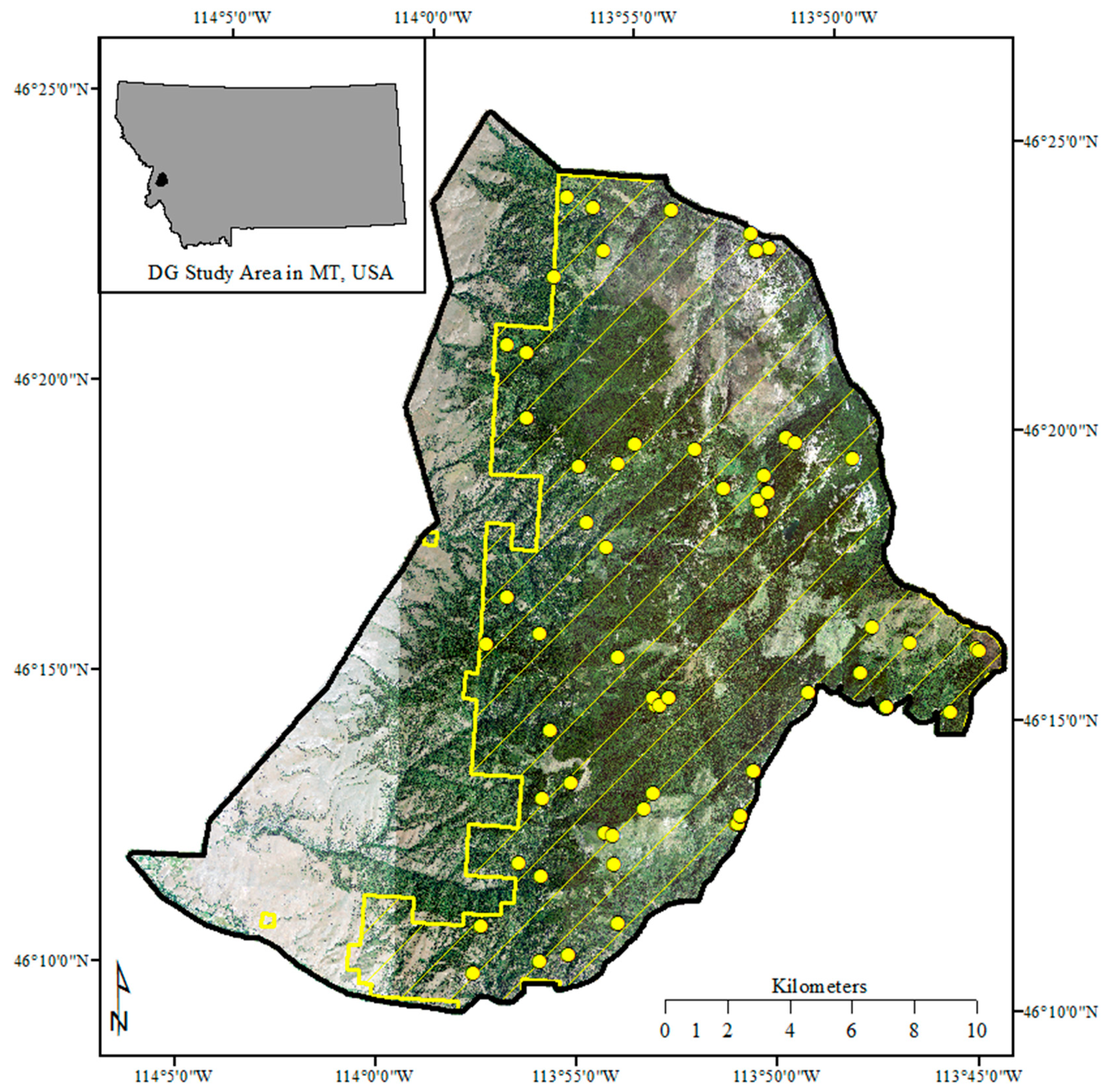
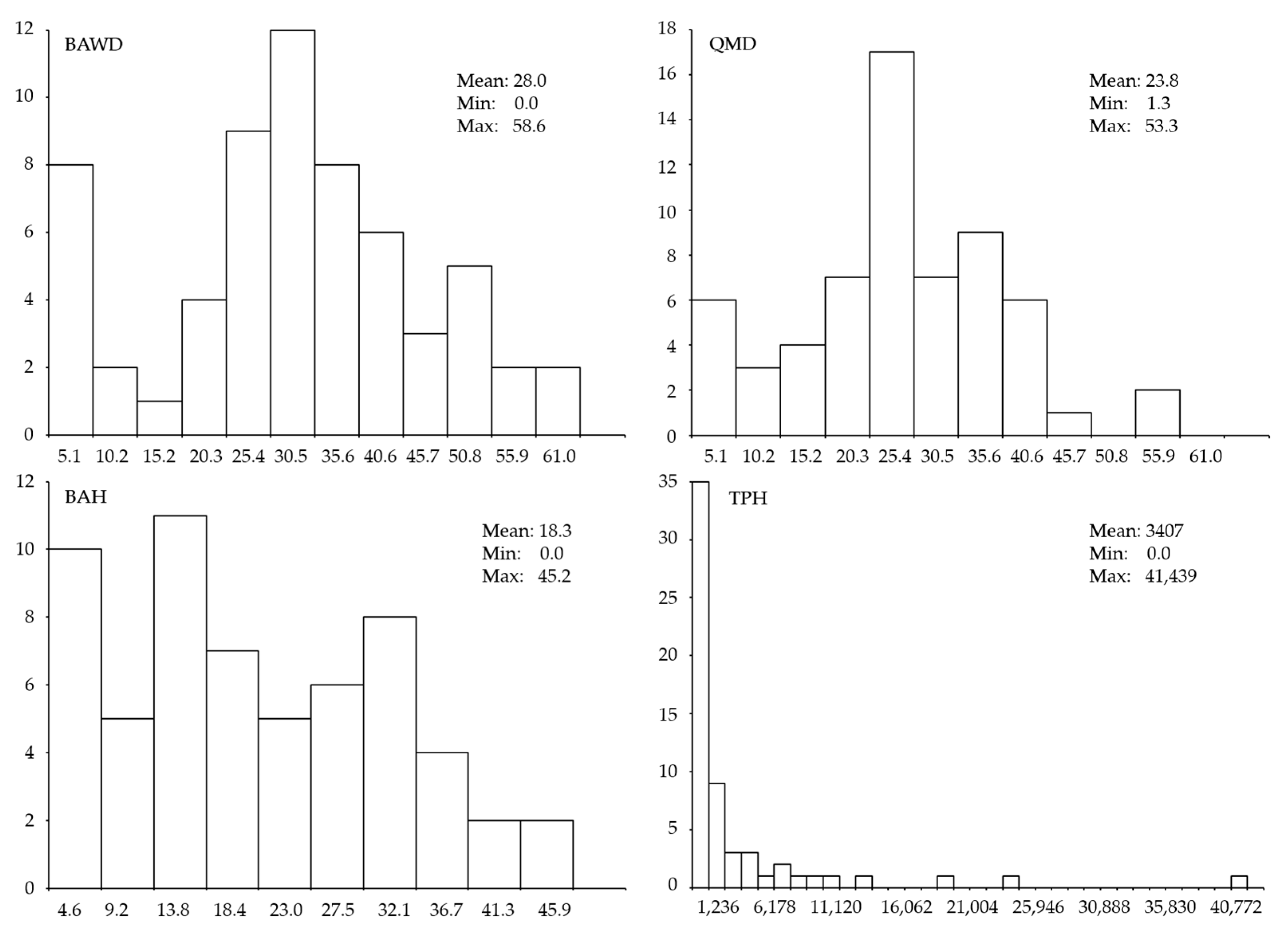
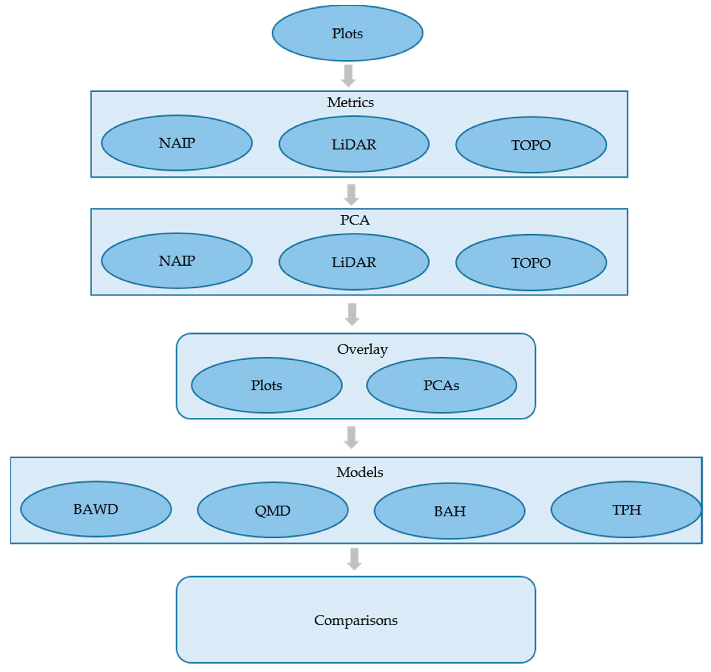
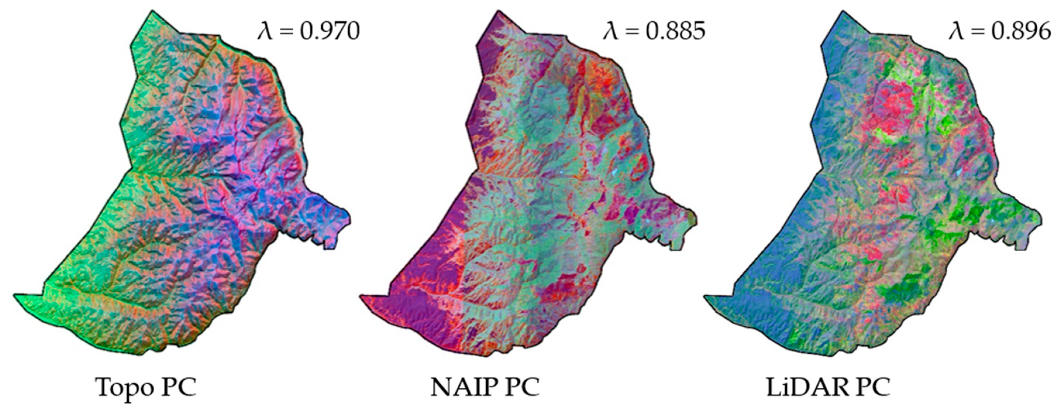
Tree data were collected on 60 plots across the study area, and tabulated to produce plot values for BAWD, QMD, BAH, and TPH. The distribution of BAWD, QMD and BAH plot values was generally considered normal while TPH values were strongly right skewed (Figure 5). Principle components used as predictor variables accounting for 96%, 97%, and 96% of the information within NAIP (5 components), TOPO (3 components) and LiDAR (5 components) data sources, respectively (Figure 6). Often Eigen vectors of a PCA are interpreted with respect to original values of the data. In this case we simply wanted to remove the correlation among each source of remotely sensed data and use the orthogonal scores of the components as predictor variables in subsequent analysis. Our PCAs effectively performed this objective. Scores calculated from the Eigen vectors of the corresponding principal components were used with plot summaries of BAWD, QMD, BAH, and TPH to build a suite of models describing the relationship between field and remotely sensed data sources. Figure 7 illustrates the spatial distribution of the multiband raster datasets generated from the principal component scores and used to produce the spatial predictions of the response variables.

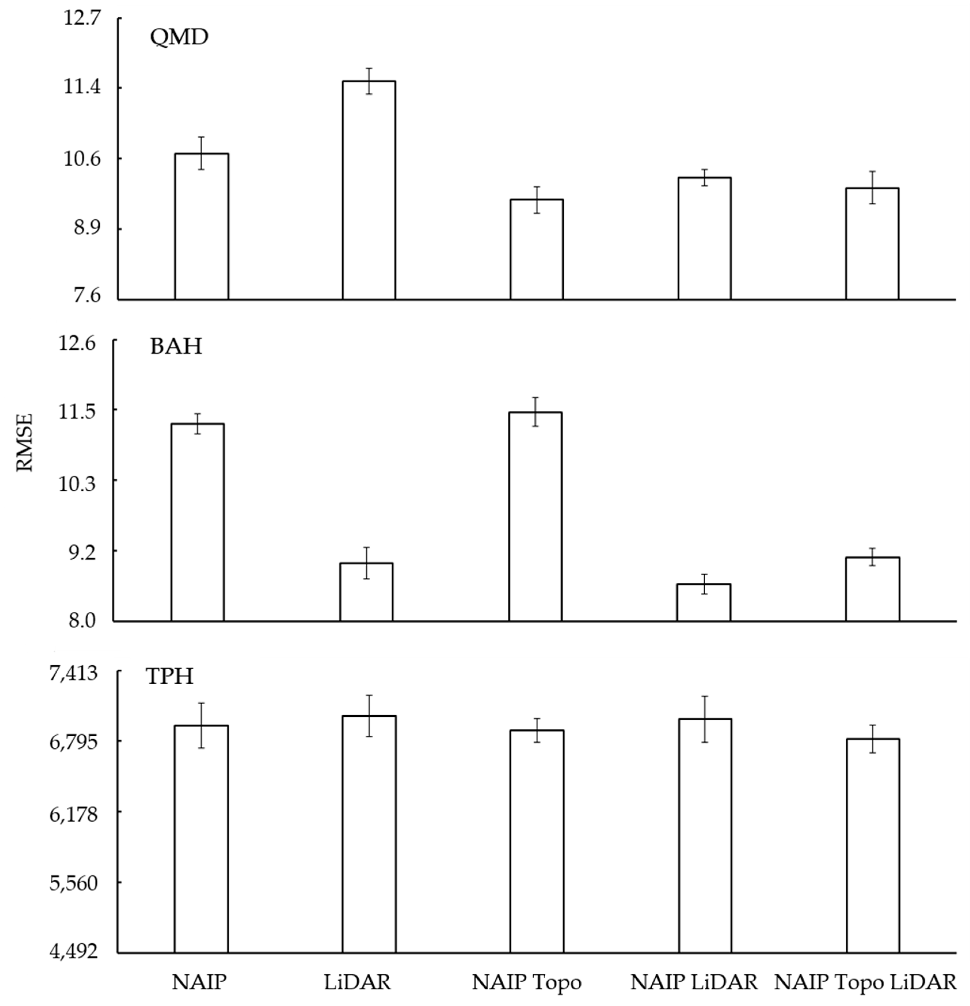
Model fit and complexity were evaluated using RMSE and AIC (

Table 2. Out of bag model fit, comparison, and rank for basal area weighted diameter (BAWD), quadratic mean diameter (QMD), basal area per hectare (BAH), and trees per hectare (TPH), where n = the number of observations, k = the number of randomly selected variables, RMSE = root mean squared error, MSE = mean squared error, AIC = Akaike Information Criterion, and ∆AIC = departure from minimum AIC score. * denotes best fitting model with the fewest number of predictor variables.

Response	Model	Variables	n	k	RMSE	MSE	AIC	Δ AIC
	1	NAIP *	60	5	12.7	161	315	0
	2	LiDAR	60	5	13.2	174	320	5
BAWD	3	NAIP TOPO	60	8	12.2	149	316	1
	4	NAIP LiDAR	60	10	11.7	137	315	0
	5	NAIP TOPO LiDAR	60	13	11.7	137	321	6
	1	NAIP	60	5	10.2	103	288	3
	2	LiDAR	60	5	11.7	137	305	20
QMD	3	NAIP TOPO *	60	8	9.4	88	285	0
	4	NAIP LiDAR	60	10	9.9	98	295	10
	5	NAIP TOPO LiDAR	60	13	9.7	93	298	13
	1	NAIP	60	5	11.2	127	300	27
	2	LiDAR *	60	5	9.0	81	273	0
BAH	3	NAIP TOPO	60	8	11.5	131	309	35
	4	NAIP LiDAR	60	10	8.6	75	279	5
	5	NAIP TOPO LiDAR	60	13	9.1	83	291	18
	1	NAIP *	60	5	6936.2	48,111,452	1071	0
	2	LiDAR	60	5	7015.3	49,214,653	1073	1
TPH	3	NAIP TOPO	60	8	6891.8	47,496,397	1077	5
	4	NAIP LiDAR	60	10	6990.6	48,868,559	1082	11
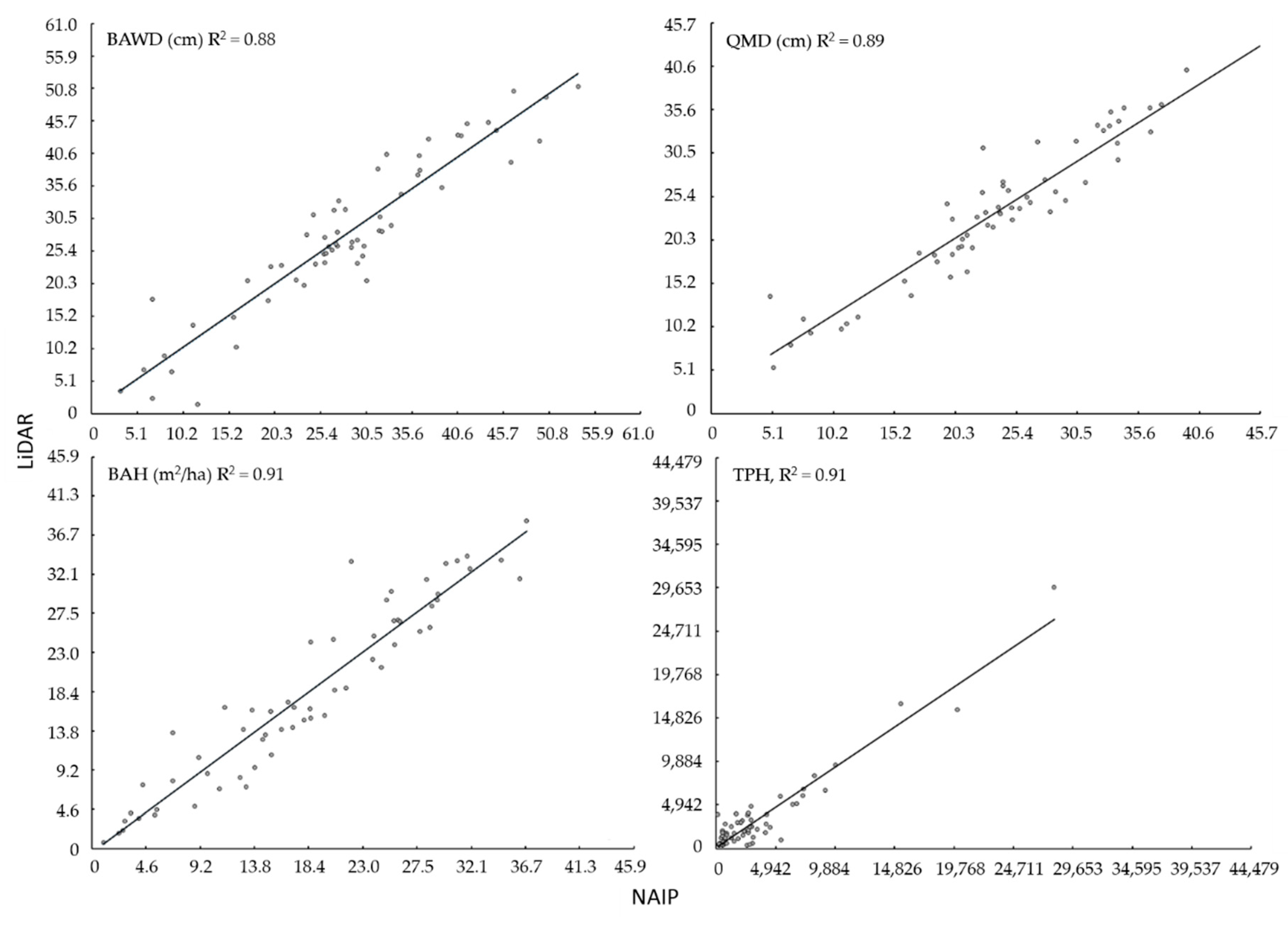
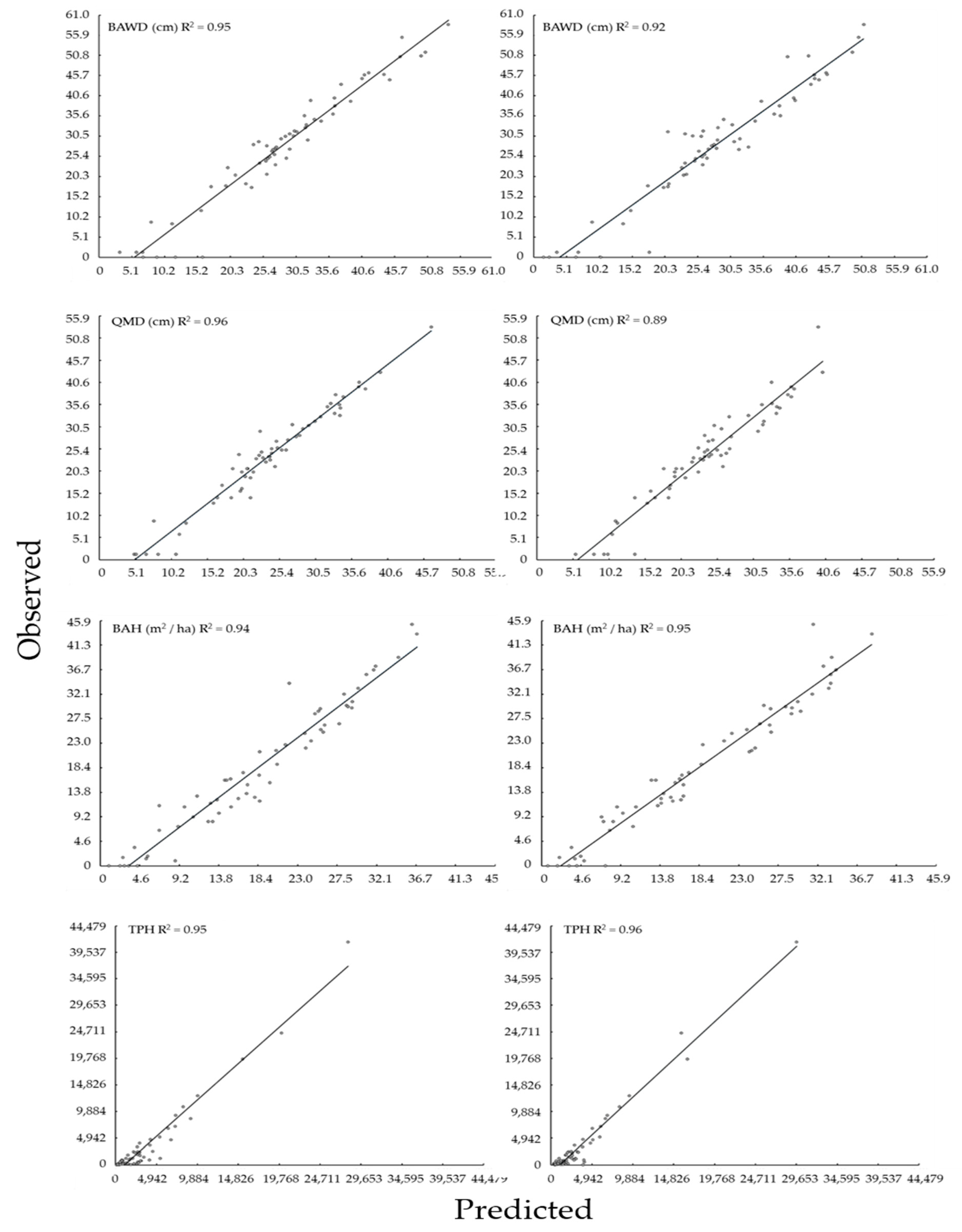
	5	NAIP TOPO LiDAR	60	13	6815.2	46,446,411	1085	14

). Generally, models derived from NAIP and LiDAR predictor variables alone performed as well as more complex models. The best fitting, most parsimonious models for BAWD, QMD, and TPH contained NAIP principal component scores. The best fitting, most parsimonious model for BAH contained LiDAR principal component scores. When estimates of BAWD, QMD, BAH, and TPH derived from NAIP and LiDAR based models were regressed against one another, they followed a positive one to one relationship explaining approximately 90% of the variation between predicted estimates (Figure 8). When paired with NAIP or LiDAR variables, TOPO variables provided little additional information.

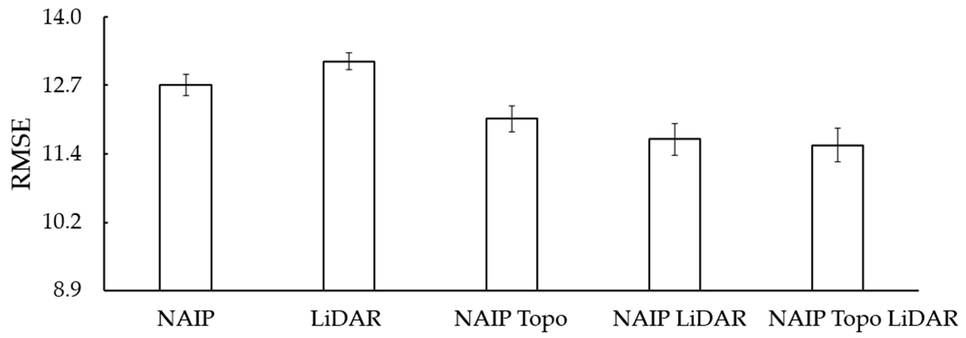
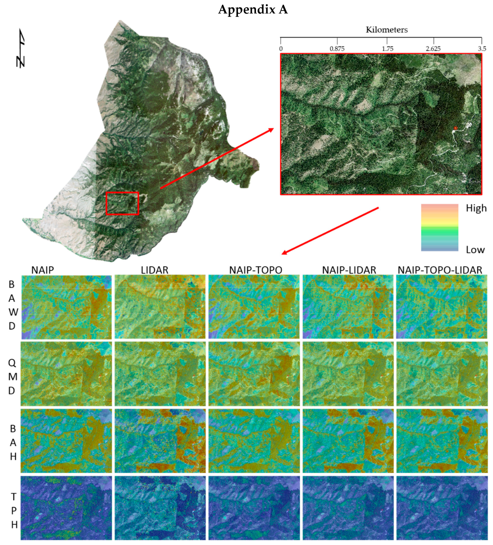
Random Forest regression model iterations yielded similar trends as shown in Table 2 but illustrate the variability of using the Random Forest ensemble modeling techniques (Figure 9). While improvements in predictive capability (smaller RMSE) can be achieved by using more complex models (Table 2 and Figure 9), those improvements are relatively minor with regard to the additional complexity (AIC scores in Table 2, Figure A1). Moreover, given the stochastic nature of ensemble modeling (Figure 9), some perceived differences in model results may be due to chance alone and was in large part the rationale for using AIC to identify the top fitting models for each characteristic.

At the stand level, differences between summarized estimates of models derived from NAIP and LiDAR are generally indistinguishable. In all comparisons except BAH, paired differences between NAIP and LiDAR derived models were statistically insignificant (

Table 3. NAIP vs LiDAR Paired t-test results for 100 summarized stand level estimates (n) of basal area weighted diameter (BAWD), quadratic mean diameter (QMD), basal area per hectare (BAH), and trees per hectare (TPH). Additional paired comparisons between models developed from combinations of NAIP, LiDAR and Topo data sources can be found in Table A2, Table A3, Table A4 and Table A5.

Characteristic	n	Difference	T-Stat	p-Value
BAWD	100	−0.119	−0.234	0.8150
QMD	100	−0.173	−0.494	0.6219
BAH	100	−2.211	−3.42	0.0009
TPH	100	128	0.464	0.6434

). For BAH, the average paired difference was less than 2.2 m² ha⁻¹ which in many surveys is roughly equivalent to one tree. Combined, these comparisons suggest that models based on NAIP and LiDAR have very similar predictive capability, error structure, and spatial distribution. This is particularly evident at the spatial scale associated with forest stands where individual pixel predictions are aggregated to produce a mean value for each stand.

4. Discussion

Forest resource managers need timely and accurate information about the size and density of trees to make decisions about what, where, and how to apply treatments across landscapes. Metrics like BAWD, QMD, BAH, and TPH are commonly used to describe structural elements of the forest. LiDAR is a relatively new technology that is capable of providing highly precise measurements of height, and has been shown as an effective tool for making spatial predictions of forest metrics by relating observed heights to ground-based plot measurements of trees [3,4].

While LiDAR data can be useful, it is not available in all locations and must generally be acquired for specific project areas [37]. Many other digital spatial datasets like topography and high resolution imagery are available as continuous data across the continental United States, and can be obtained free of charge. Like LiDAR data, recent research has also shown that fine resolution imagery such as NAIP can be used to effectively predict forest metrics with relationships based on field data.

Alone, neither NAIP nor LiDAR data can model environmental phenomenon without high quality, reliable reference information. In this study, 60 field plots following the CSE protocol were used to describe a range of forest conditions. While this field protocol is commonly used for forest inventories, it may not be optimal for relating ground measurements to fine resolution spatial data such as NAIP imagery or LiDAR [38].

Without adequate ground representation of the characteristics to be estimated, good model fit cannot be achieved. This was evident in the relatively large RMSE between measured and estimated TPH in our study. To enhance our ability to estimate and map forest characteristics, a sufficient number of plots should be collected to cover the range of conditions across the study area. Those plots should also be designed to fully describe the entire area of the plot. Future research on appropriate plot layout and configuration with regard to predictor variables is needed to better understand these relationships, and improve the predictive ability of forest metric modeling.

For many natural resource management questions, collection of training data can be one of the expensive and important aspects of a project. When data collection saving can be made by using readily available, and free, remotely sensed data in lieu of purchasing new data, it may be beneficial to use those savings on collecting robust training datasets. With more time and resources available for training data collection, the spatial distribution of trainings sites may be enhanced, or more thorough measurements may be taken at each site, depending on project specific needs. Whether more information is collected at each site, or more sites are added to a set, better training data generally lead to better fitting models and ultimately, reduced uncertainly, enhanced predictive ability, and more confident decision making.

Using the relationships derived from our field plots and remotely sensed data, we demonstrated that there was a great deal of similarity between NAIP and LiDAR based model estimates at the spatial scale of a plot and forest stand. In most of our comparisons models that used NAIP based predictors out performed those that used LiDAR or TOPO. In some cases, using both NAIP and LiDAR based predictors showed minor improvements in model fit. Often those improvements though were small and from a model complexity stand point there was no justification for adding additional sources of data, especially sources of data that have additional acquisition costs. Assuming that acquisition cost of remotely sensed data is a key factor to quantifying forest characteristics for the sake of forest management decision making, in our study the added cost of acquiring LiDAR data to estimate BAWD, QMD, BAH, or TPH was not worth the marginal improvement in estimating those characteristics at the spatial scale of the plot and stand.

Cost, quality, continuity, and time are all essential components to consider when quantifying forest characteristics. Our analyses suggest that outputs from models based on NAIP or LIDAR at the spatial scale of the plot and stand compare favorably. Thus, using imagery or elevation-based data to generate estimates of the forest metrics described in this study is somewhat irrelevant. If one source of data is available, there is not much to be gained by spending time or money to acquire an additional source. However, full coverage image data tends to be more readily available than LiDAR, which is currently only collected in isolated patches. Furthermore, when time is of the essence, it must be understood that custom acquisition of remotely sensed data, whether imagery or LIDAR, can be time consuming and may significantly delay a project.

For other forest characteristics related to topography and understory vegetation we presume that airborne LiDAR based models would have a substantial advantage over passive based imagery in accurately quantifying those characteristics. However, our study focused on quantifying common overstory components of the forest used in forest management decision making. In this instance, with the exception of BAH, LiDAR based models did not substantially improve estimates of BAWD, QMD, or TPH. Moreover, when comparing modeled estimates of BAH, especially at the spatial scale of the forest stand, it is highly questionable if the added cost of LiDAR acquisition is worth the minor reduction in modeled error. This has leads us to suggest that when existing remotely sensed data is available such as NAIP and additional resources are available for quantifying overstory forest characteristics, more emphasis on field data collection and design may prove to be a better use of those financial resources than purchasing additional remotely sensed data.

5. Conclusions

Both NAIP and LiDAR were used independently and in combination to predict the spatial distribution of forest characteristics such as BAWD, QMD, BAH, TPH. While recent attention has been focused on using LiDAR data to estimate these characteristics, we have shown that, when using common modeling techniques, similar results can be obtained by using high resolution imagery (NAIP). Therefore, either type of data could be used to perform these analyses and produce equivalent results when estimates of size and density are of interest. This is particularly apparent when fine grain, spatially explicit raster estimates are summarized to larger units such as forest stands.

Interestingly, NAIP and LiDAR measure different aspects of the environment, and when trees and forest characteristics are considered they both provide disparate but useful information for describing BAWD, QMD, BAH, and TPH. Our modeling results show that although different predictor layers (NAIP versus LiDAR) are being used to estimate forest characteristics, each output yields relatively similar interpretations of the forest. We show that regardless of whether NAIP or LiDAR is used, they both have equivalent predictive ability, error structure, and spatial distribution. Given the similarity in predicting forest metrics from these sources of data, using NAIP is a low-cost alternative to using LiDAR.

References

1. Sheridan, R.D.; Popescu, S.C.; Gatziolis, D.; Morgan, C.L.S.; Ku, N.W. Modeling forest aboveground biomass and volume using airborne LiDAR metrics and forest inventory and analysis data in the Pacific Northwest. Remote Sens. 2015, 7, 229–255. [Google Scholar] [CrossRef]
2. Mitchell, B.; Jacokes-Mancini, R.; Fisk, H.; Evans, D. Considerations for Using Lidar Data—A Project Implementation Guide; RSAC-10032-MAN1; USDA Forest Service, Remote Sensing Applications Center: Salt Lake City, UT, USA, 2012; 13p.
3. McRoberts, R.E.; Naesset, E.; Gobakken, T. Inference for lidar-assisted estimation of forest growing stock volume. Remote Sens. Environ. 2013, 128, 268–275. [Google Scholar] [CrossRef]
4. Moser, P.; Vibrans, A.C.; McRoberts, R.E.; Naesset, E.; Gobakken, T.; Chirici, G.; Mura, M.; Marchetti, M. Methods for variable selection in LiDAR-assisted forest inventories. Forestry 2017, 90, 112–124. [Google Scholar] [CrossRef]
5. USDA Farm Service Agency. Four Band Digital Imagery Information Sheet. 2016. Available online: https://www.fsa.usda.gov/Assets/USDA-FSA-Public/usdafiles/APFO/support-documents/pdfs/fourband_infosheet_2016.pdf (accessed on 14 February 2017).
6. Hogland, J.; Anderson, N.; Wells, L.; Chung, W. Estimating forest characteristics using NAIP imagery and ArcObjects. In Proceedings of the 2014 ESRI International Users Conference, San Diego, CA, USA, 9–13 August 2004. [Google Scholar]
7. Hogland, J.; Anderson, N. Estimating FIA plot characteristics using NAIP imagery, function modeling, and the RMRS Raster Utility coding library. In Pushing Boundaries: New Directions in Inventory Techniques and Applications: Forest Inventory and Analysis (FIA) Symposium 2015, Portland, Oregon, 8–10 December 2015; Stanton, S.M., Christensen, G.A., Eds.; General Technical Report PNW-GTR-931; U.S. Department of Agriculture, Forest Service, Pacific Northwest Research Station: Portland, OR, USA, 2015; pp. 340–344. [Google Scholar]
8. Hogland, J.; Anderson, N. Function modeling improves the efficiency of spatial modeling using big data from remote sensing. Big Data Cogn. Comput. 2017, 1, 3. [Google Scholar] [CrossRef]
9. Hogland, J.; Anderson, N.; St. Peters, J.; Drake, J.; Medley, P. Mapping Forest Characteristics at Fine Resolution Across Large Landscapes of the Southeastern United States Using NAIP Imagery and FIA Field Plot Data. Int. J. Geo-Inf. 2018, 7, 140. [Google Scholar] [CrossRef]
10. Haralick, R.; Shanmugam, K.; Dinstein, J. Texture features for image classification. IEEE Trans. Syst. Man Cybern. 1973, 3, 610–621. [Google Scholar] [CrossRef]
11. Gesch, D.; Oimoen, M.; Geenlee, S.; Nelson, C.; Steuck, M.; Tyler, D. The National Elevation Dataset. Photogramm. Eng. Remote Sens. 2002, 68, 5–11. [Google Scholar]
12. Aerial Photography Field Office (APFO). Imagery Programs. 2018. Available online: https://www.fsa.usda.gov/programs-and-services/aerial-photography/imagery-programs/index (accessed on 17 December 2018).
13. Sugarbaker, L.; Eldridge, D.; Jason, A.; Lukas, V.; Saghy, D.; Stoker, J.; Thunen, D. Status of the 3D Elevation Program; U.S. Geological Survey Open-File Report 2016–1196; U.S. Geological Survey: Reston, VA, USA, 2015; 13p.
14. Akaike, H. Information theory and an extension of the maximum likelihood principle. In Proceedings of the 2nd International Symposium on Information Theory; Petrov, B.N., Csaki, F., Eds.; Akadémiai Kiadó: Budapest, Hungary, 1973; pp. 267–281. [Google Scholar]
15. Akaike, H. A new look at the statistical model identification. IEEE Trans. Autom. Control 1974, 19, 716–723. [Google Scholar] [CrossRef]
16. Thornton, P.E.; Thornton, M.M.; Mayer, B.W.; Wei, Y.; Devarakonda, R.; Vose, R.S.; Cook, R.B. Daymet: Daily Surface Weather Data on a 1-km Grid for North America, Version 3; ORNL DAAC: Oak Ridge, TN, USA, 2013. Available online: http://0-dx-doi-org.brum.beds.ac.uk/10.3334/ORNLDAAC/1328 (accessed on 25 January 2017).
17. Burns, R.; Honkala, B. Silvics of North America: 1. Conifers; 2. Hardwoods; Agriculture Handbook 654, Tech. Coords; U.S. Department of Agriculture, Forest Service: Washington, DC, USA, 1990; Volume 2, 877p.
18. Freese, F. Elementary Forest Sampling; Agriculture Handbook No. 232; USDA Southern Forest Experiment Station, Forest Service: Knoxville, TN, USA, 1973. Available online: https://www.fs.fed.us/fmsc/ftp/measure/cruising/other/docs/AgHbk232.pdf (accessed on 25 January 2017).
19. USDA Forest Service. Region One Vegetation Classification, Mapping, Inventory and Analysis Report 16-5 v6.0. Region 1 Common Stand Exam and Inventory and Monitoring Field Guide. 2016. Available online: http://fsweb.r1.fs.fed.us/forest/inv/cse_exams/R1_CSE_IM_FG_v2016.zip (accessed on 25 January 2017).
20. Holden, Z.A.; USDA Forest Service. Region 1 Regional Office, Forest and Rangeland Management, 26 Fort Missoula Rd. Missoula, MT 59804, USA. Personal communications, 2016.
21. USDA Farm Service Agency. National Agriculture Imagery Program (NAIP) Information Sheet. 2015. Available online: https://www.fsa.usda.gov/Assets/USDA-FSA-Public/usdafiles/APFO/ naip_info_sheet_2015.pdf (accessed on 25 January 2017).
22. USDI Geological Survey. File Transfer Protocol. Staged NAIP, 2018. Available online: ftp://rockyftp.cr.usgs.gov/vdelivery/Datasets/Staged/NAIP/ (accessed on 9 March 2018).
23. USDI Geological Survey. File Transfer Protocol. Staged NED, 2018. Available online: ftp://rockyftp.cr.usgs.gov/vdelivery/Datasets/Staged/NED/ (accessed on 9 March 2018).
24. Watershed Sciences. LiDAR Remote Sensing Collection: USFS Bitterroot National Forest, Montana; Delivery 2 October 29, 2010; Watershed Science: Corvallis, OR, USA, 2010; Available online: https://quantumspatial.com/ (accessed on 8 January 2018).
25. McGaughey, R.J. FUSION/LDV: Software for LIDAR Data Analysis and Visualization; USDA Forest Service, Pacific Northwest Research Station: Washington, DC, USA, 2016. Available online: http://forsys.cfr.washington.edu/fusion/ FUSION_manual.pdf (accessed on 25 January 2017).
26. Souza, C. A Tutorial on Principal Component Analysis with Accord.NET Framework; Technical Report; Department of Computing, Federal University of Sao Carlos: São Carlos, Brazil, 2012; Available online: http://arxiv.org/ftp/arxiv/papers/1210/1210.7463.pdf (accessed on 27 September 2013).
27. Breiman, L. 2001. Random forests. Mach. Learn. 2001, 45, 5–32. [Google Scholar] [CrossRef]
28. Liaw, A.; Wiener, M. Classification and regression by randomForest. R News 2002, 2, 18–22. Available online: http://CRAN.R-project.org/doc/Rnews/ (accessed on 25 January 2017).
29. Liaw, A. Documentation for R Package randomForest. 2015. Available online: https://cran.r-project.org/web/packages/randomForest/randomForest.pdf (accessed on 25 January 2017).
30. USDA Forest Service. Geospatial Data: Northern Region Existing Vegetation Mapping Program. 2016. Available online: https://www.fs.usda.gov/detailfull/r1/landmanagement/gis/?cid=stelprdb5331054& width=full (accessed on 25 January 2017).
31. Barber, J.; Brown, S.R.; Ahl, R. Mid-Level and Base-Level Databases of the R1 Existing Vegetation (VMap) Products; Region One Vegetation Classification, Mapping, Inventory and Analysis Report; USDA Forest Service: Washington, DC, USA, 2016; pp. 12–38. Available online: https://www.fs.usda.gov/Internet/FSE_DOCUMENTS/ stelprdb5364531.pdf (accessed on 25 January 2017).
32. Ahl, R.; Brown, S. The Bitterroot and Lolo National Forests Region 1 Existing Vegetation Database (VMap) Revision of 2016; Northern Region Geospatial Group Project Report NRGG-PR-BITLO-VMAP2016; USDA Forest Service: Washington, DC, USA, 2017. Available online: https://www.fs.usda.gov/Internet/FSE_DOCUMENTS/ fseprd573432.pdf (accessed on 5 March 2017).
33. Avery, T.; Burkhart, H. Forest Measurements, 4th ed.; McGraw Hill: Boston, MA, USA, 1994; p. 408. [Google Scholar]
34. Smith, D.; Larson, B.; Kelty, M.; Ashton, P. The Practice of Silviculture Applied Forest Ecology, 9th ed.; John Wily & Sons, Inc.: New York, NY, USA, 1997; p. 537. [Google Scholar]
35. Bush, R. Overview R1 Summary Database; Region One Vegetation Classification, Mapping, Inventory and Analysis Report 14-16 v2.0; USDA Forest Service: Washington, DC, USA, 2014. Available online: http://fsweb.r1.fs.fed.us/forest/inv/r1_tools/Overview_R1_SDB.pdf (accessed on 25 January 2017).
36. Bush, R.; Reyes, R.; Zeiler, J.D. R1 Summary Database Reports and Utilities User’s Guide; Region One Vegetation Classification, Mapping, Inventory and Analysis Report 16-2 v3.2; USDA Forest Service: Washington, DC, USA, 2016. Available online: http://fsweb.r1.fs.fed.us/forest/inv/r1_tools/R1_SDB_Rep_Util.pdf (accessed on 25 January 2017).
37. Mitchell, B.; Walterman, M.; Mellin, T.; Wilcox, C.; Lynch, A.M.; Anhold, J.; Falk, D.A.; Koprowski, J.; Laes, D.; Evans, D.; et al. Mapping Vegetation Structure in the Pinaleno Mountains Using Lidar-Phase 3: Forest Inventory Modeling; RSAC-10007-RPT; USDA Forest Service, Remote Sensing Applications Center: Salt Lake City, UT, USA, 2012; 17p.
38. Mundt, J.T.; Streutker, D.R.; Glenn, N.F. Mapping sagebrush distribution using fusion of hyperspectral and lidar classifications. Photogramm. Eng. Remote Sens. 2006, 72, 47–54. [Google Scholar] [CrossRef]
Figure 1. Daly-Gold Study Area in the Sapphire Mountains of the Bitterroot National Forest in western Montana, USA is shown. The yellow linear features describe the National Forest Systems administrative boundary and the land within it, and the yellow point features illustrate the location of plots and associated field measurements used in this study.
Ijgi 08 00024 g001
Figure 2. Composition and structure of common stand exam plot design, with outer circle (orange) representing a 0.04 hectare plot for trees greater than or equal to 12.7 cm diameter at breast height (radius = 11.4 m) and inner circle (yellow) representing a 0.0013 ha plot for trees less than 12.7 cm DBH (radius = 2 m). The outer square represents the area summarized for the NAIP imagery and LiDAR data.
Ijgi 08 00024 g002
Figure 3. Flow diagram of the data sources, processing steps, modeling, and comparisons made within the study. NAIP, LiDAR, and TOPO data were converted to texture, height, and elevation metrics and transformed to spatial surfaces using principal component analysis (PCA). PCA surface values were then related to field data based on plot locations (Overlay) and were used to model basal area weighted diameter (BAWD), quadratic mean diameter (QMD), basal area per hectare (BAH) and trees per hectare (TPH) relationships. Modeled relationships were then used to create raster surfaces that were compared at the spatial resolution of the plot and stand.
Ijgi 08 00024 g003
Figure 4. Daly-Gold Study Area lifeform classification with randomly selected forest polygons highlighted in black. Summarized metric predictions were compared in these polygons.
Ijgi 08 00024 g004
Figure 5. Distribution of basal area weighted diameter (BAWD), quadratic mean diameter (QMD), basal area per hectare (BAH), and trees per hectare (TPH) collected on 60 plots within the study area.
Ijgi 08 00024 g005
Figure 6. Principal component graph, where LiDAR is solid black, NAIP is dashed, and TOPO is dotted. The solid horizontal line indicates the minimum 95% threshold of the cumulative variation that is explained by the number of principal components.
Ijgi 08 00024 g006
Figure 7. Illustration of TOPO, NAIP, and LiDAR principal component raster datasets. Note that only the first three components are displayed by the red-green-blue-color composite. The proportion of correlation explained (λ) by those components is display above each raster dataset.
Ijgi 08 00024 g007
Figure 8. Linear relationship between basal area weighted diameter (BAWD), quadratic mean diameter (QMD), basal area per hectare (BAH), and trees per hectare (TPH) estimates derived from NAIP and LiDAR models (Table 1). Observed versus predicted values for NAIP and LiDAR based BAWD, QMD, BAH, and TPH are given in Figure A2.
Ijgi 08 00024 g008
Figure 9. Variation in out of bag root mean squared error (RMSE) for 10 basal area weighted diameter Random Forest models. Results for quadratic mean diameter, basal area per hectare, and trees per hectare are given in Figure A3.
Ijgi 08 00024 g009