Deep Learning Segmentation and 3D Reconstruction of Road Markings Using Multiview Aerial Imagery

Abstract

The 3D information of road infrastructures is growing in importance with the development of autonomous driving. In this context, the exact 2D position of road markings as well as height information play an important role in, e.g., lane-accurate self-localization of autonomous vehicles. In this paper, the overall task is divided into an automatic segmentation followed by a refined 3D reconstruction. For the segmentation task, we applied a wavelet-enhanced fully convolutional network on multiview high-resolution aerial imagery. Based on the resulting 2D segments in the original images, we propose a successive workflow for the 3D reconstruction of road markings based on a least-squares line-fitting in multiview imagery. The 3D reconstruction exploits the line character of road markings with the aim to optimize the best 3D line location by minimizing the distance from its back projection to the detected 2D line in all the covering images. Results showed an improved IoU of the automatic road marking segmentation by exploiting the multiview character of the aerial images and a more accurate 3D reconstruction of the road surface compared to the semiglobal matching (SGM) algorithm. Further, the approach avoids the matching problem in non-textured image parts and is not limited to lines of finite length. In this paper, the approach is presented and validated on several aerial image data sets covering different scenarios like motorways and urban regions.

1. Introduction

The availability of large-scale, accurate high-resolution 3D information of roads with lane markings and road infrastructure plays an important role towards autonomous driving. Aerial imagery is a valuable database to derive 3D information of roads even in areas difficult to access, like on motorways. Driven by the development of autonomous driving, area-wide, high-resolution 3D information of the road surfaces, including lane markings, is necessary, as well as new methods to derive this information from aerial imagery, as shown in Reference [1]. The standard work flow using aerial images would be to project the images onto a digital surface model (DSM) and to derive the information in the projected imagery, but the generation of DSMs from stereo images is challenging in regions with low textures. The lane markings, for example, are the most visible texture on asphalt roads useful for 3D reconstruction. Thus, it is desired to improve the quality of the DSM on road surfaces by exploiting the line character of the lane markings.

Several approaches have been proposed for the 3D reconstruction of line features from multiview airborne optical imagery. Studies in References [2,3,4] tried to match line segments based on their appearances or some additional geometry constraints. Schmid and Zisserman [2] exploited the epipolar geometry of line segments and the one-parameter family of homographies to provide point-wise correspondences. However, standard appearance-based matching approaches for 3D reconstruction are hardly applicable on lane markings due to the similar color profile of all road markings and the lack of textures in their neighboring areas. In Reference [1], a new method for 3D reconstruction of road markings was proposed without the need for an explicit line matching. This method exploits the line character of road markings with the aim to optimize the best 3D line location by minimizing the distance from its back projection to the detected 2D line in all the covering images. The road markings were detected by a geometrical line detector, which produces many false positives. Road masks produced by road databases are applied to reduce the error rates.

The automatic segmentation of road markings by a specifically designed algorithm for this task based on a modified fully convolutional neural network was addressed in Reference [5]. The network was trained on the AerialLane18 data set [5] which contains 20 aerial images from the 3K sensor system [6] with a GSD (ground sampling distance) of 13 cm. The overall accuracy is specified with $77.7\%$ IoU based on the given test data set.

In this paper, the two aforementioned approaches were integrated in the new proposed approach for automatic segmentation and 3D reconstruction of road markings using multiview aerial imagery. The accuracy of road marking segmentation will be further improved by exploiting the multiview character of the aerial images and the 3D reconstruction approach was slightly modified in terms of the integration of road marking segments instead of detected lines. A road masking is not necessary anymore and the whole work flow does not require any 3rd-party information. Further, the whole approach was tested on several data sets covering different scenarios like motorways, rural roads, parking places, and urban roads. Experimental data were acquired on 29 March 2017 from the DLR (German Aerospace Center) helicopter BO-105 covering 100 km of the motorway A9 north of Munich and 10 km of urban roads in the north of Munich. The GSD of the aerial images ranges between 7 cm and 12 cm. For our experiments, four areas were selected covering all mentioned scenarios.

2. Road Marking Properties

The challenges in automatic road marking segmentation are abrasion, changing illumination conditions, like brightness and strong shadows caused by trees and buildings, as well as partial or total occlusion by other objects, such as bridges or tree branches. The appearance of lane markings on German roads, including line type, color, and width, is quite manifold and depends on the road type. Different line types of lane markings with their line widths are listed in

Table 1. Geometry of lane markings (selection).

		Motorways	Rural Roads	Other Roads
	continuous line (narrow width)	$0.15$ [m]	$0.12$ [m]	$0.12$ [m]
	continuous line (broad width)	$0.30$ [m]	$0.25$ [m]	$0.25$ [m]
	dashed line (length/gap)	$12.0$/$6.0$ [m]	$4.0$/$8.0$ [m]	$3.0$/$6.0$ [m]
	double line (distance)	$0.15$ [m]	$0.12$ [m]	$0.12$ [m]

. The dashed lane markings have, for example, 6 m length and a gap length of 12 m on motorways. On other road types, distances are shorter. The widths of road markers are also defined, but as illustrated in Figure 1a, there are divergences from the definition in practice, e.g., the line width is $0.8$ m instead of $0.3$ in some regions. In addition, many special markings are allowed, e.g., barrier markings like in Figure 1b.

In Figure 1, the challenge to derive 3D information of road markings using only aerial images is illustrated, as the standard SGM (semiglobal matching) process has significantly more noise on road surfaces compared to regions with more texture. For each aerial image (Figure 1a–c), the corresponding parts of the DSM (Figure 1d–f) are pictured, showing noisy heights for the road surface.

3. Methodology

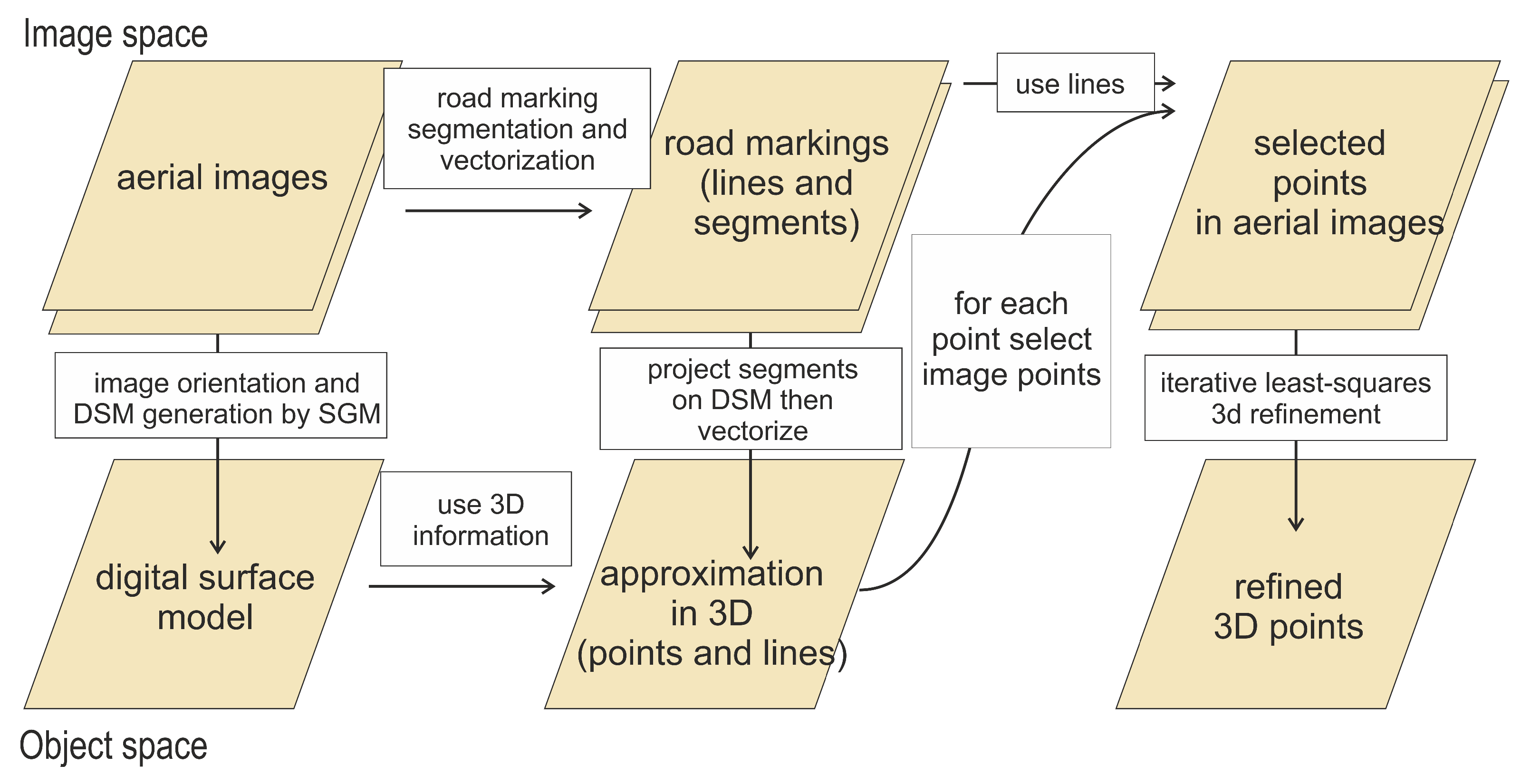
In this section, the methodology of selected processing steps for automatic segmentation and 3D reconstruction using multiview aerial imagery based on the work flow shown in Figure 2 is described. The work flow can be divided into image space and object space operations. The work flow starts with the aerial images, from which a DSM was generated and the road markings were segmented. Based on the segmented road markings and the DSM, approximation points can be derived in the object space. The last step starts with the selection of points in the aerial images for each approximation point, with which the 3D refinement will be fed.

In the following subsections, the most important operations are depicted: Deep-learning-based segmentation of road markings (Section 3.1), the least-squares refinement of 3D points (Section 3.2), and the generation of approximations as well as selection of corresponding line points (Section 3.3). Other processing steps, like DSM generation, are described in the Experimental section (Section 4).

3.1. DL (Deep Learning) Segmentation of Road Markings

In order to localize road markings (lane markings), we applied a deep learning algorithm based on an improved version of the algorithm proposed by the authors of [5]. To localize the lane markings, previous methods mostly applied two-step algorithms. First, a binary road segmentation method was applied to create a road mask, then non-learning-based algorithms were used to localize the lane markings. The masking of road segments reduces the high false positive rate in non-road areas. However, Azimi et al. [5] proposed a single-step learning-based algorithm for the first time, to the best of our knowledge, to localize the lane markings directly by learning their features.

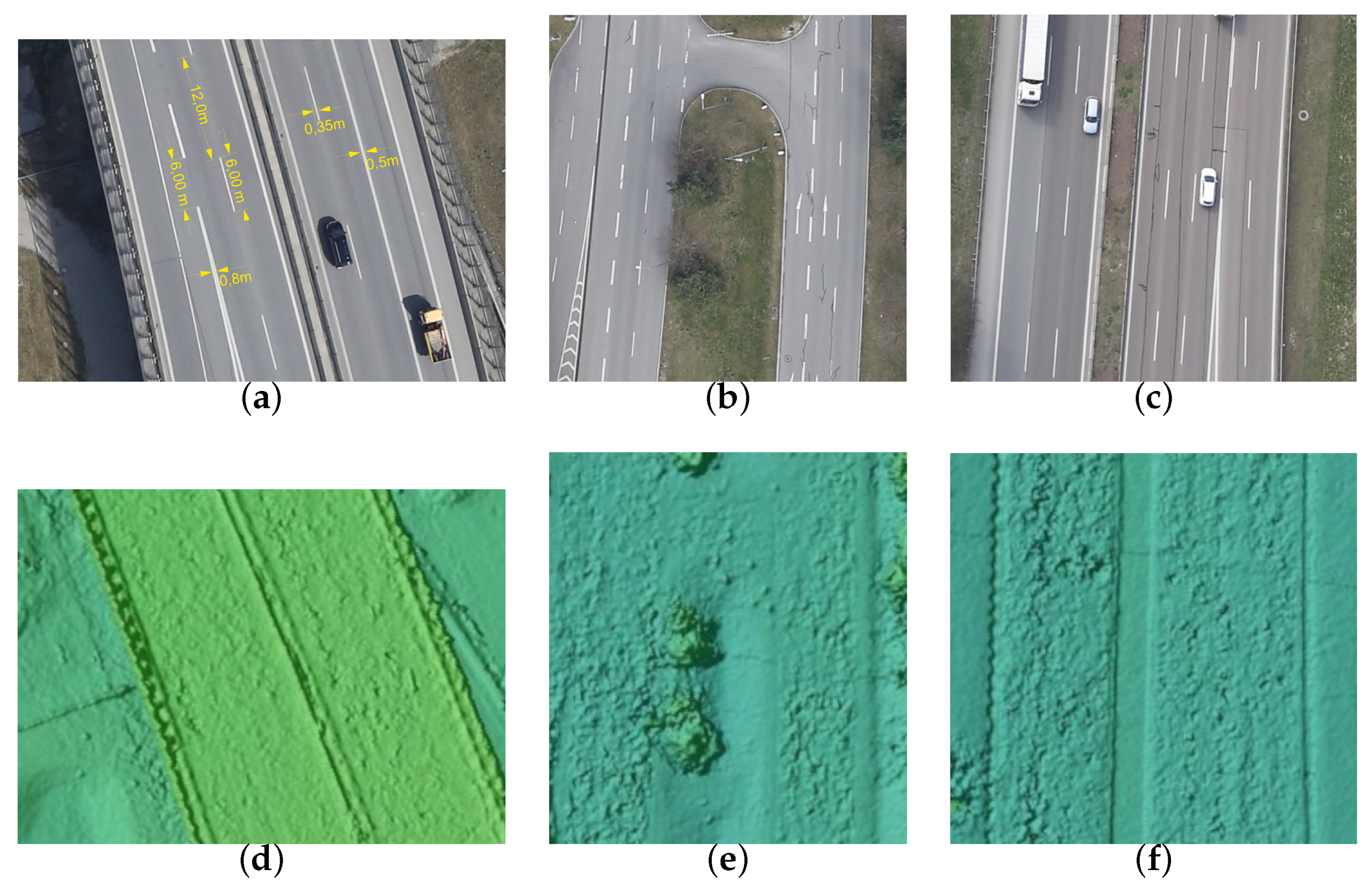
In order to use deep learning methods, an annotated data set is necessary. Therefore, a pixel-wise lane marking segmentation data set was created using airborne imagery, called the AerialLanes18 data set. They used images acquired by the 3K sensor system [6]. The images were acquired over the city of Munich on the 26 April 2012 with a GSD of 13 cm.

Since lane markings in aerial images appear as tiny patterns, the direct application of deep learning algorithms will lead to a poor performance, e.g., based on patterns of 1 × 1 pixel size. The reason for this is the low-spectral analysis capability in CNNs (convolutional neural networks). Therefore, a method based on a modified fully CNN enabling a full spectral analysis will provide better performance.

In this article, the proposed DL algorithm was again trained with the AerialLanes18 data set, but here, a cleaned version of the data set was used. The architecture of the network is composed of two parts, an encoder and a decoder. The encoder extracts the high semantic, but lower resolution features from input data and the decoder recovers the original resolution from the output of the encoder. Wavelet transformations are used in combination with the CNN, allowing a full-spectral analysis of input images, which is important when it comes to tiny object segmentation, like lane markings. In this work, residual blocks have been used in the network architecture to further improve the performance.

To apply the modified neural network, the images were first chopped to the size of $512\times 512$ pixel. Afterwards, each patch was fed to the network as input. As output, a binary pixel-wise mask was obtained, containing predicted pixels for lane and non-lane marking classes. In the last step, a customized stitching algorithm was applied, considering the fact that CNNs have lower performance in boundary regions, which is assumed to be caused by the receptive field of the network.

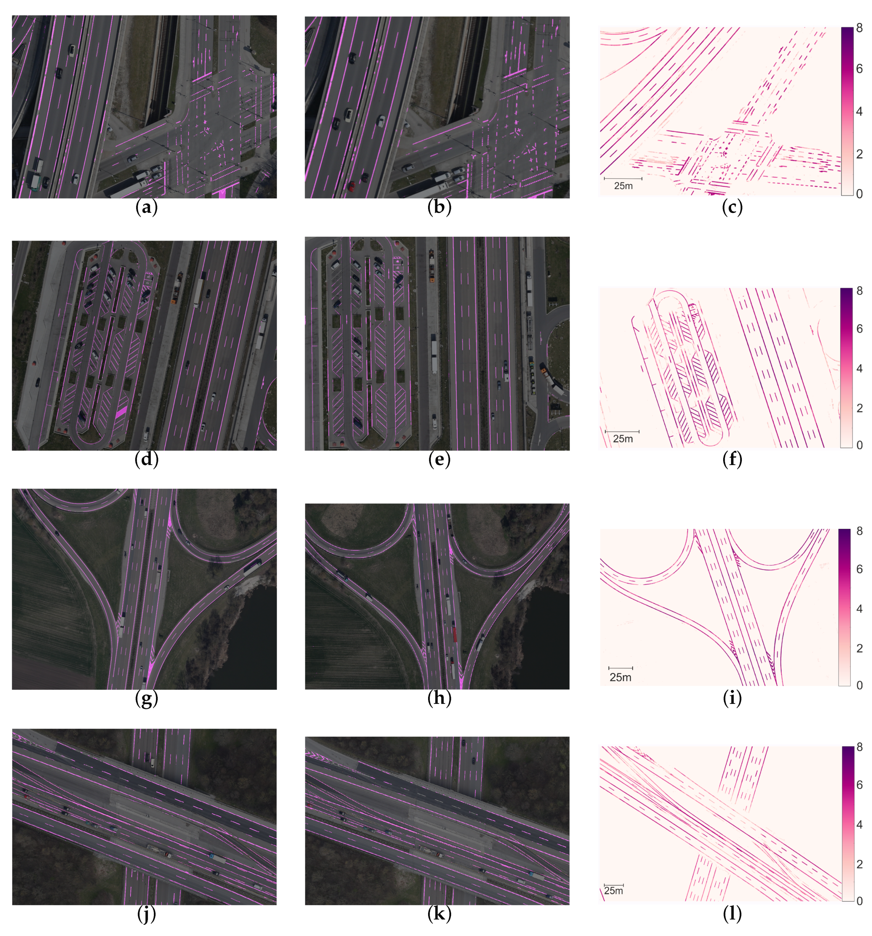
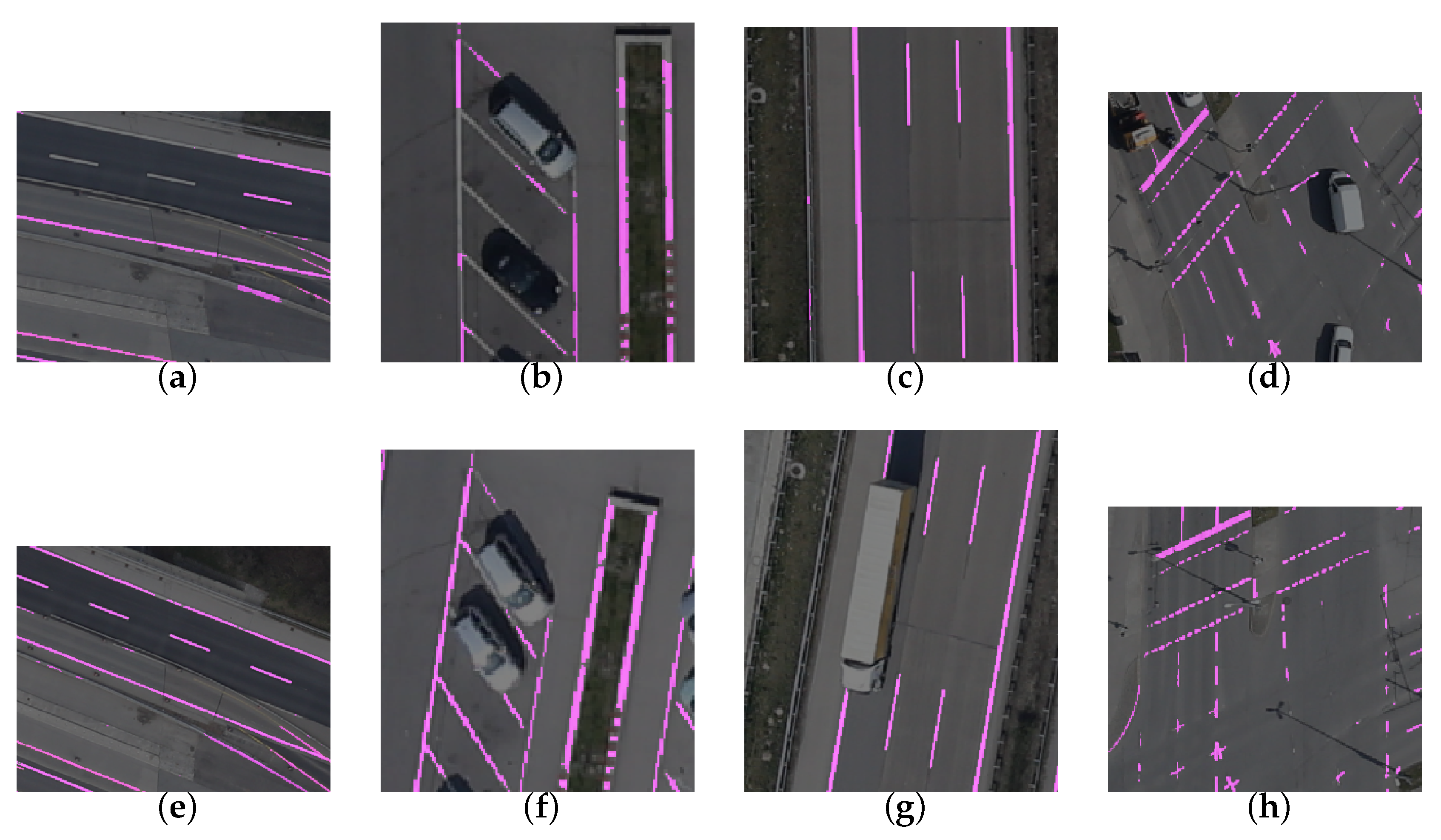
It should be emphasized once again that the whole work flow is independent of any 3rd party information, such as OpenStreetMaps or Google Maps, and allows us to localize road markings with their 3D information regardless of their location with pixel-wise accuracy. It is also capable of localizing different road marking types, such as long, dash, no parking, and zebra lines, and different symbols, such as turn, speed-limit, bus, bicycle, and disabled signs.

The accuracy of the algorithm is expected to be higher on dark road surfaces, because the AerialLanes18 data set contains mostly roads with dark surfaces. Therefore, expanding the data set to contain roads with stretched contrasts between lane markings and road surfaces would improve the performance. For more information, we refer to Azimi et al. [5].

3.2. Least-Squares Refinement of 3D Points

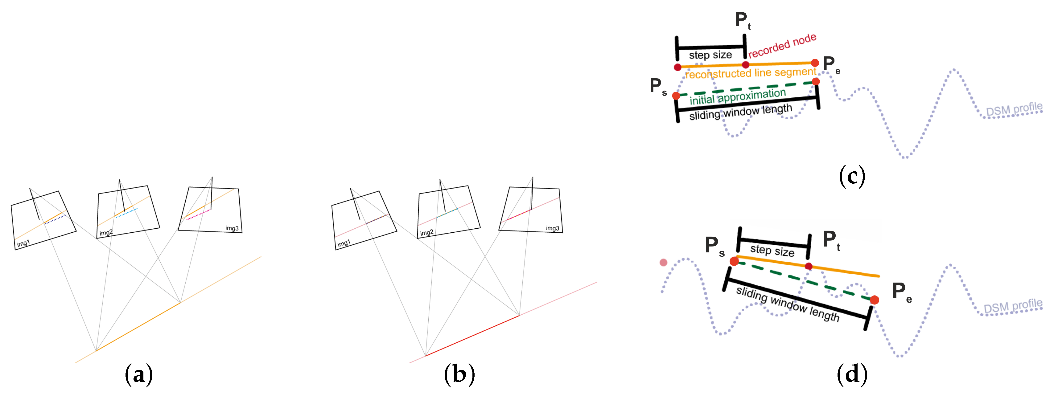
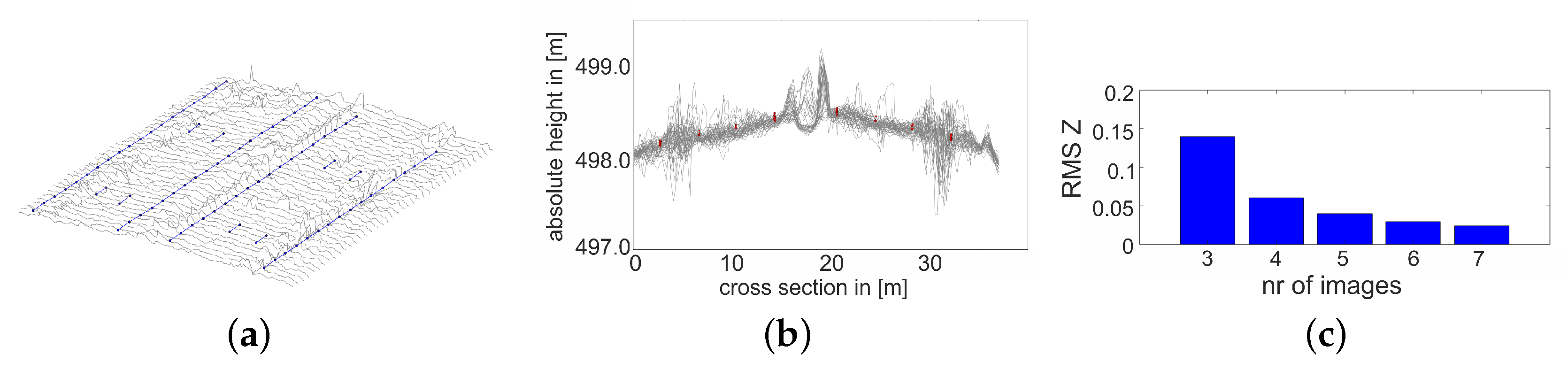
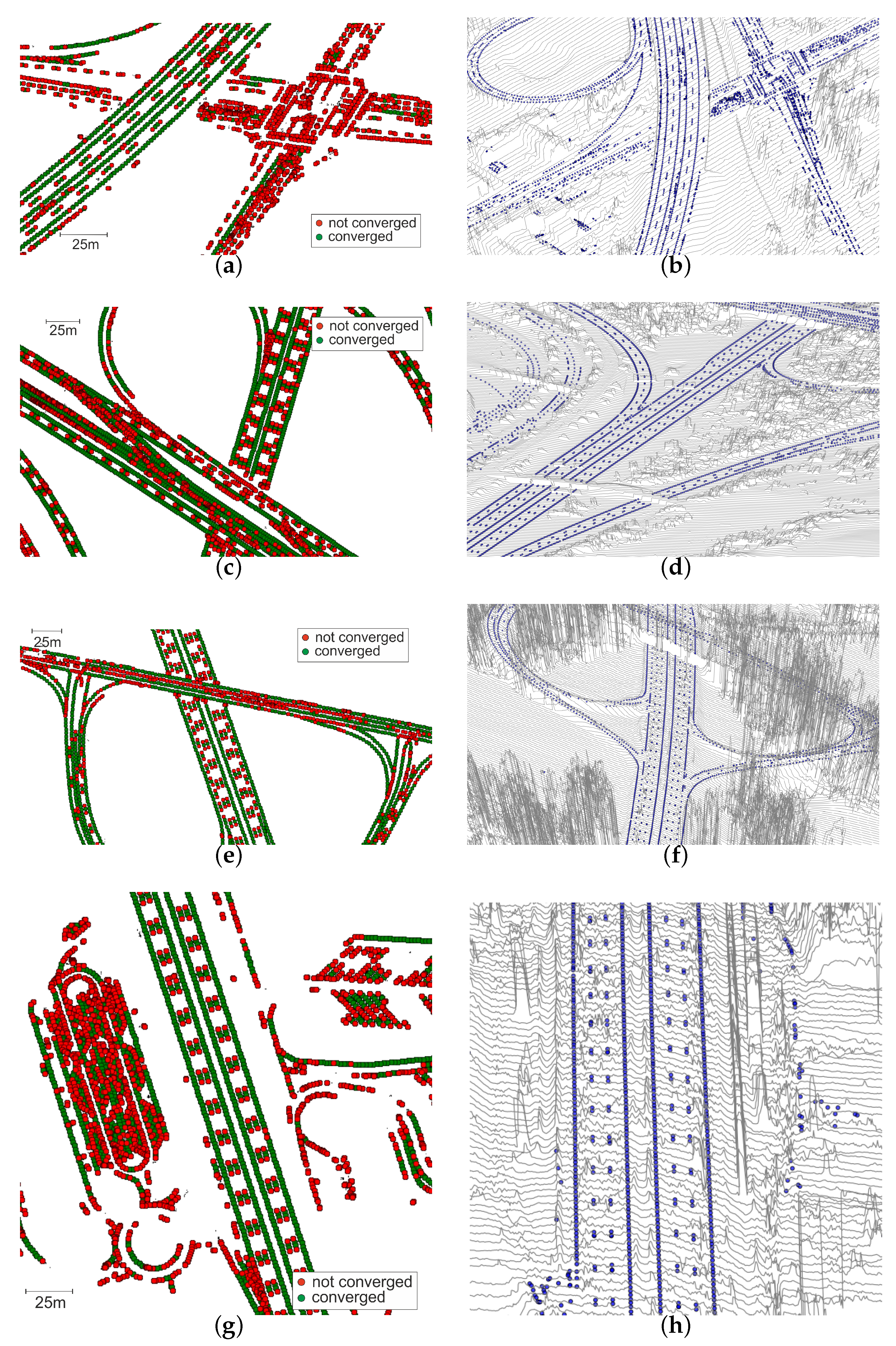
In this section, the process of refining the 3D position of a point at a road marking is described, as illustrated in Figure 3. Following Taylor’s idea on minimization of a objective function [7], we define an orthogonal regression function to optimize the 3D position of each point in the object space so that its back projection would best fit the detected lines in all the covering views (see Figure 3a,b). Thus, the position and height of each 3D lane marking segment will be refined in one optimization step. The proposed approach addresses the challenging (quasi) infinite and curved properties of lane markings in the 3D reconstruction by applying a sliding window iteration of length $2·S$ defined by a start point ${\mathbf{P}}_{\mathbf{s}}(X_s,Y_s,Z_s)$, an end point ${\mathbf{P}}_{\mathbf{e}}(X_e,Y_e,Z_e)$, and S as step size. The 3D coordinates of the start and end point are estimated by the least-squares process and the target point ${\mathbf{P}}_{\mathbf{t}}(X_t,Y_t,Z_t)$ coordinates in the center are then recorded afterwards. After this, the sliding window moves to the next point. Starting from the recorded node of previous process, another line segment is reconstructed, i.e., the sliding window has moved step size forward. Its center point is then recorded and the step is repeated.

The orthogonal regression in the image space is defined as follows. Let the image coordinates of start and end point on the regression line be $(x_s,y_s)$ and $(x_e,y_e)$ where $y_e\ne y_s$, and the observed image points (here: The skeleton points of segmented road markings) be $\{x_i,y_i\}$ for $i=1\dots N$ with N as the number of points. The observed image points have errors $e_{x_i}$ and $e_{y_i}$. The orthogonal regression model in two-point form is then:

$$x_i-e_{x_i}=x_s+{\displaystyle \frac{(x_e-x_s)}{(y_e-y_s)}}·(\overline{y_i}-y_s)$$

(1)

$$y_i-e_{y_i}=\overline{y_i}.$$

(2)

To express (1) and (2) shortly, a function $\mathcal{F}$ is defined as:

$$\widehat{{\mathbf{p}}_i}=\mathcal{F}({\mathbf{p}}_s,{\mathbf{p}}_e,{\overline{y}}_i),$$

(3)

which takes the image coordinates of the start point ${\mathbf{p}}_{\mathbf{s}}(x_s,y_s)$ and end point ${\mathbf{p}}_{\mathbf{e}}(x_e,y_e)$ in the image space as well as the predicted y-coordinate $\overline{y_i}$ of an image point $\mathbf{p}({\overline{x}}_i,{\overline{y}}_i)$ and returns the estimated image coordinates $\widehat{\mathbf{p}}(\widehat{x},\widehat{y})$ on $\overline{{\mathbf{p}}_{\mathbf{s}}{\mathbf{p}}_{\mathbf{e}}}$.

For the setup of the least-squares functions, observation and constraint equations must be defined. They describe the fitting of straight lines defined by the approximation start and end point to the extracted lines in all covering images, where the fitting lines on different images are transformed from a single line segment in the object space through the extended collinearity equation. Regarding the fact that the collinearity is a point-wise condition, a line segment is represented by the start and end point ${\mathbf{P}}_s(X_s,Y_s,Z_s)$ and ${\mathbf{P}}_e(X_e,Y_e,Z_e)$ in the object space.

Given a start point ${\mathbf{P}}_s$ and an end point ${\mathbf{P}}_e$ of a line segment m in the object space and the interior and exterior parameters ${\mathbf{q}}^j$ of image j, where $j\le J$, with J as the number of images covering this line segment, the back projection of these points into image j then results in the image coordinates ${\mathbf{p}}_s^j(x_s^j,y_s^j)$ and ${\mathbf{p}}_e^j(x_e^j,y_e^j)$.

$$\begin{array}{c}\hfill {\mathbf{p}}_s^j=\mathcal{G}({\mathbf{q}}^j,{\mathbf{P}}_s)\\ \hfill {\mathbf{p}}_e^j=\mathcal{G}({\mathbf{q}}^j,{\mathbf{P}}_e)\end{array}$$

(4)

Let m be the corresponding line segment on image j, where $m\le M$, with M as number of lines being extracted (observed). Given a data set $\{x_{m,i}^j,y_{m,i}^j\}$ of point i on line segment m in image j, their estimated image coordinates ${\widehat{\mathbf{p}}}_{m,i}^j$ on the infinite line $\overline{{\mathbf{p}}_s^j,{\mathbf{p}}_e^j}$ derived from the orthogonal regression model (Equation (3)) are then:

$${\widehat{\mathbf{p}}}_{m,i}^j=\mathcal{F}({\mathbf{p}}_s^j,{\mathbf{p}}_e^j,y_{m,i}^j).$$

(5)

Combining Equations (4) with (5) gives function $\mathcal{H}$:

$${\widehat{\mathbf{p}}}_{m,i}^j=\mathcal{F}(\mathcal{G}({\mathbf{q}}^j,{\mathbf{P}}_s),\mathcal{G}({\mathbf{q}}^j,{\mathbf{P}}_e),y_{m,i}^j)=\mathcal{H}({\mathbf{q}}^j,{\mathbf{P}}_s,{\mathbf{P}}_e,y_{m,i}^j),$$

(6)

which takes image interior and exterior parameters ${\mathbf{q}}^j$, the object coordinates of ${\mathbf{P}}_s$ and ${\mathbf{P}}_e$, which define a line $\overline{{\mathbf{P}}_s,{\mathbf{P}}_e}$, and the observed y-coordinate of the point ${\mathbf{p}}_{m,i}^j$ in image space, and returns the estimated image coordinates ${\mathbf{p}}_{m,i}^j$ on the back projected line of $\overline{{\mathbf{P}}_s,{\mathbf{P}}_e}$. Following the structure of the Gauss–Markov model, they are expressed as:

$$\mathit{b}+\widehat{\mathit{v}}=\mathit{f}\left(\widehat{\mathit{x}}\right):{\mathbf{p}}_{m,i}^j+{\widehat{\mathit{v}}}_{m,i}^j=\mathcal{H}({\mathbf{q}}^j,{\widehat{\mathbf{P}}}_s,{\widehat{\mathbf{P}}}_e,{\widehat{y}}_{m,i}^j),$$

(7)

with the amount of observations ${\displaystyle o=2·\sum N^j}$ and with the amount of unknowns ${\displaystyle u=6+\sum N^j}$.

To make the least-squares system robust and to avoid singularities, three constraint equations are defined. The first two equations are to fix the X- and Y-coordinates of the start point using the approximate values. This has influence on the very first estimation, as the start point has to be fixed to the approximation values. In the following steps of the sliding window, the estimated middle point can be used as fixed start point. The third equation is the fixation of the length of the line segment (i.e., constraining the relative location of the end point), which avoids unnecessary movements of the line end point. Following the structure of the Gauss–Markov model with constraints $\mathit{h}\left(\widehat{\mathit{x}}\right)=\mathbf{0}$, all constraint equations can be written as:

$$\left[\begin{array}{c}{\widehat{X}}_s-{X_s}^0\\ {\widehat{Y}}_s-{Y_s}^0\\ \sqrt{{({\widehat{X}}_s-{\widehat{X}}_e)}^2+{({\widehat{Y}}_s-{\widehat{Y}}_e)}^2+{({\widehat{Z}}_s-{\widehat{Z}}_e)}^2}-2\ast S\end{array}\right]=\left[\begin{array}{c}0\\ 0\\ 0\end{array}\right],$$

(8)

with the number of constraints $c=3$. The redundancy of the problem is then:

$${\displaystyle r=o+c-u=\sum N^j-3.}$$

(9)

Two kinds of singular cases can happen. First, a configuration defect in the object space appears, if there is no intersection of at least two projection rays possible as the 3D reconstruction approach still relies on the intersection of multiple projection rays from different views. This happens if there is only one image covering the area or all line segment lay on epipolar lines. In these cases, the problem is not solvable. Second, a configuration defect in image space can happen, when all or nearly all of the extracted lines lie in row direction on all the covering images. In all other cases, e.g., if the targeted line segments lie only on some of the stereo pairs’ epipolar planes, the problem is still solvable, as those stereo pairs are not contributing to the solution. The same shall apply if only in some of the images, the extracted line segments lie in row direction: The problem is solvable, as those images are not contributing measurements to the estimation. In practice, no configuration defects occur, as the special flight configuration described in Section 4.1 will prevent the occurrence.

More details about the implemented Gauss–Markov model with constraints, including some sensitivity and simulation studies can be found in Reference [1]. The resulting 3D coordinates of the target point ${\mathbf{P}}_{\mathbf{t}}(X_t,Y_t,Z_t)$ are simply calculated as the geometric center of start and end point.

3.3. Generation of Approximations and Selection of Corresponding Line Points

The task here is to select observed points ${\mathbf{p}}_{m,i}^j$ on line m in image j as defined in Equation (7), given a start and end point ${\mathbf{P}}_{\mathbf{s}}$ and ${\mathbf{P}}_{\mathbf{e}}$ in object space. The starting point is the road marking segments in the covering images, as well as the orthoprojected segments in the object space. With projecting all images onto the DSM, the segmented labels will be superimposed in the object space, i.e., if one point of the road marking is missed in one image, it may be detected in the other images and thus result in a higher confidence.

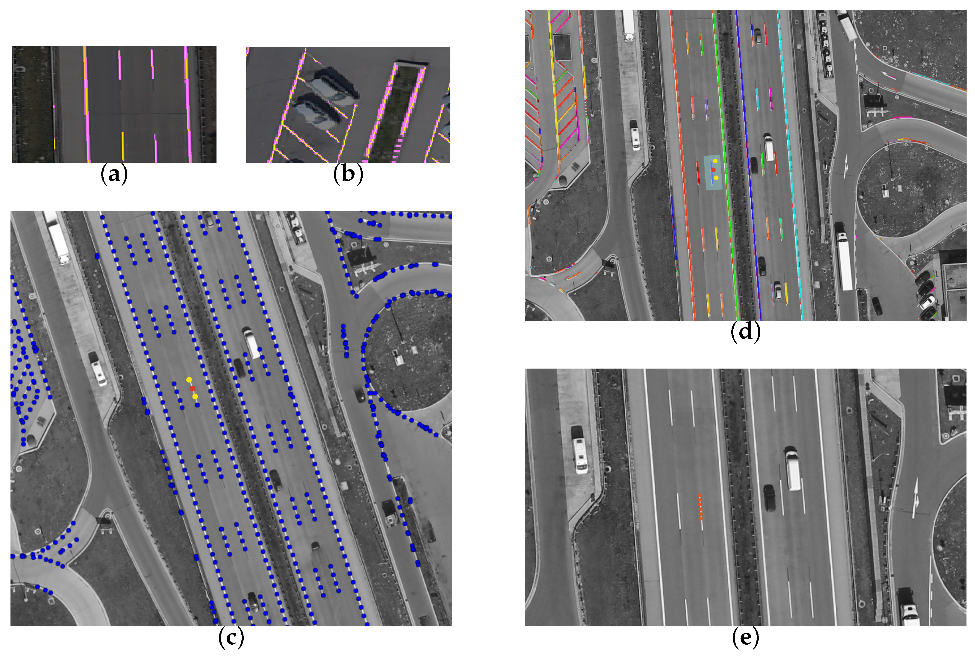
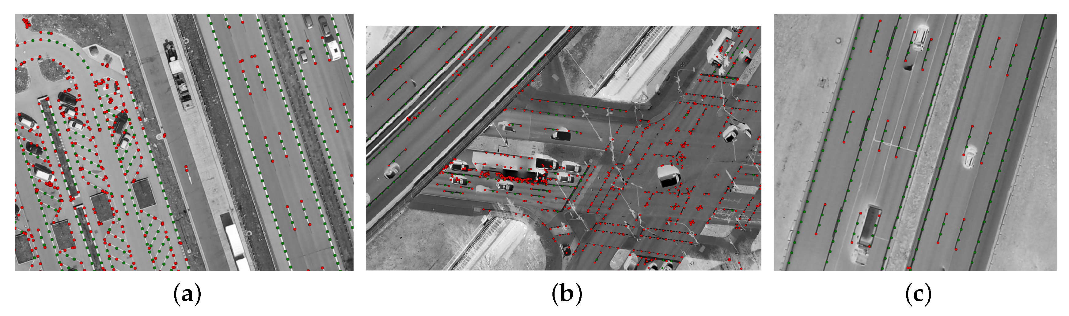
The whole process of selecting image points and generating approximation points is visualized in Figure 4. Given the road marking segments in the images, a skeleton operator is performed, which extracts the center lines of the road marking segments (see Figure 4a,b). After pruning and smoothing of the center lines, the center points are recorded. 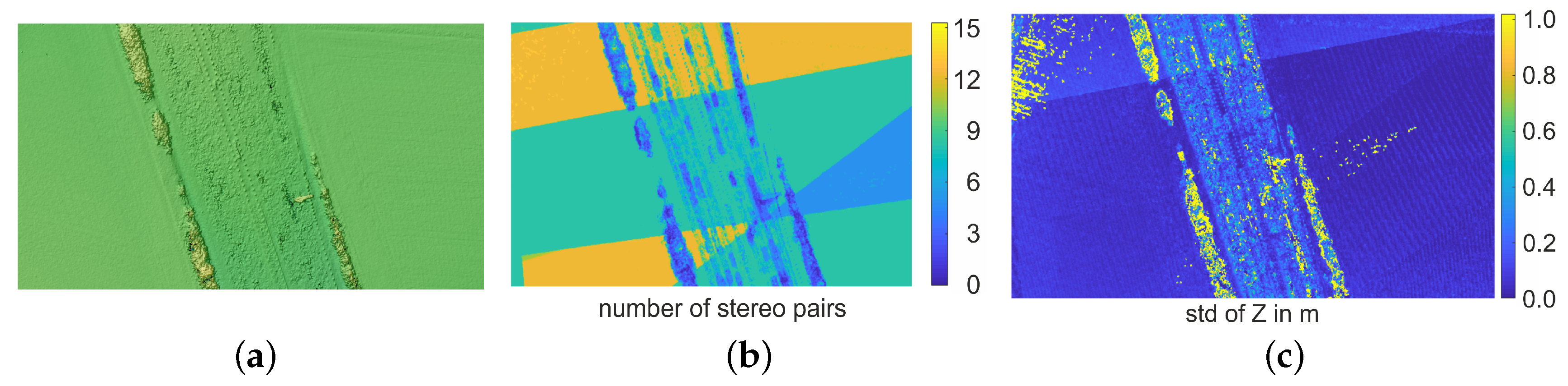Additionally, approximation points are generated for each line based on the Euclidean distance of step size S using the labels in the orthoprojected images. The X and Y values are derived from the orthoprojection of the original image onto the DSM, whereas the Z value is taken from the DSM directly, which finally gives approximations for start, end, and target points as visualized in Figure 4c.

By back-projecting the start and end points into each image, the corresponding line points can be found, which is a crucial step, as the assignment can be ambiguous due to inaccurate approximation values or missing line detection. This step is visualized in Figure 4d. A search space around the back-projected start and end points must be defined, in which all points are assumed to belong to the same line. Additional checks are required in terms of parallelism, distances, and straightness to avoid wrong assignments, which finally leads to many rejected points. However, a parameter defining the size of the search space must be defined, which is the distance of observed line point to the line between the back-projected start and end point in pixel. This parameter depends, among others, on the GSD of images and road marking sizes. Finally, all the observed road marking points for each image are collected as shown in Figure 4e. Based on this procedure, there is no need for a direct point or line matching between the images, as the points on each line are collected independently in each image.

4. Experimental Results and Evaluations

The approach was tested and validated on four sets of aerial images covering different scenarios, urban roads, motorways, rural roads, and parking spaces. The input data and test setups are described in Section 4.1. The DSM generation and some preprocessing steps are presented in Section 4.2. The result chapter is divided in the results of the DL segmentation (Section 4.3) and the results of the 3D refinement (Section 4.4).

4.1. Input Data

The aerial images were acquired with the DLR 4k sensor system [8] operated on the helicopter BO105. The helicopter pilots were instructed to fly each route twice, once on one side and once on the other of a motorway. This special flight configuration as illustrated in

Table 2. (a) Flight trajectory of DLR helicopter. The green line shows the flight trajectory. Source: Google Earth 4 January 2018. (b) Properties of the 4k camera system aboard the helicopter. (c) Flight configuration.

	(b)
		Canon EOS 1D-X
	Lenses Sensor/Pixel size Image size	Zeiss M. Planar f/2.0 50 mm Full frame CMOS/6.944 μm 5184 × 3456 pixel, ratio 3:2 (17.9 MPix)
	(c)
		Flight Configuration
	Oblique angle FOV Coverage @500m Flight height GSD @500-700m Across overlap Along overlap	±15° ±34° across strip, ±13° along strip 780 m × 230 m 500–700 m 7–9 cm (nadir) 50% 75%

is designed to cover up long distances and in the same turn to guarantee a stereo view for each point on the motorway, with a minimum of required images. This is in comparison to the classical photogrammetric approach on flight planning, with several straight flight lines to cover the whole motorway in a stereo view.

The in-house-developed 4k system provides oblique aerial images acquired with two Canon EOS 1D-X cameras. The oblique viewing angle is $\pm 15°$ across flight track. The pixel size is around $6.9$ $\mathsf{\mu }$m, which leads, in combination with the focal length 50 mm and flying height $H_{flight}$ between 500 and 700 m above ground, to a GSD between 7 and 9 cm in nadir direction. All important parameters with respect to the camera and flight configuration are listed in Table 2. The across and along overlap of $50\%$ resp. $75\%$ leads to a eightfold image coverage of each point on the motorway.

The aerial images were georeferenced by global navigation satellite system GNSS/Inertial system IGI AEROcontrol-IId and further improved by the satellite positioning service of the German national survey (SAPOS) correction. Together with the camera calibration, the interior and exterior parameters for each image were given and are further improved by a bundle adjustment. Details are described in References [1,6].

In principle, the proposed approach works from here without any additional information. In application, additional ground information can be introduced to further improve the absolute geolocation accuracy. As described in Reference [9], aerial imagery can be further improved to have an absolute geolocation accuracy of better than 30 centimeters if TerraSAR-X geodetic points are included as reference points. Additionally, a global terrain model (like from X-Band Shuttle Radar Topography Mission (SRTM)) can be introduced to tie the derived DSM heights to the level of the global terrain model. In this article, the absolute geolocation accuracy was not analyzed and validated. Instead, the aim was to compare the relative accuracies derived from the SGM generated DSM with the 3D refined points of this approach. The absolute geolocation accuracy plays no role in the validation, as both cases depend on the same geolocation and accuracy level.

The image acquisition flight took place on 29 March 2017 along the motorway A9 starting from Munich, Germany, going 100 km northbound. For further analysis, altogether 111 from around 4000 images were selected from this flight covering (A) urban roads, (B) motorways, (C) rural roads, and (D) parking spaces. Area A covers 1.1 × 1.2 km${}^2$ with 23 images, area B 1.0 × 2.2 km${}^2$ with 42 images, area C 1.0 × 1.5 km${}^2$ with 23 images, and area D 1.0 × 1.4 km${}^2$ with 23 images. In one image of each scenario, all road markings were labelled manually for later validation of DL segmentation. The manually labelled road markings were orthoprojected onto the DSM, which was used as the ground truth for the validation of the multiview segmentation (see Section 4.3).

4.2. DSM Generation

For further processing, all observed image positions and attitudes were improved by a self-calibrating least-squares bundle adjustment. As there were no ground control points available, the bundle adjustment received the necessary pass information from a reference surface model (X-Band SRTM), which provided approximate heights for each tie point. In the adjustment step, the interior camera parameters, like focal length, principal point, and lens distortion parameters, were also estimated to reach the required accuracies for DSM processing. With this, the final height level of the DSM is tied to the level of the shuttle radar topography mission (SRTM) DEM. The RMSE of the tie point’s coordinates was between 0.1–0.3 m for all data sets. Subsequently, an SGM-based process chain like in Reference [10] was carried out by distributed grid computing generating dense 3D points that could be used to reconstruct the observed earth surface.

In the data sets A to D, the matching precision of SGM was estimated to be about 0.5 pixel [11], which leads to a lower accuracy level than in the tie point matching. This can partly be improved by averaging the heights in the large number of overlapping stereo pairs, but in areas with low textures or repeating patterns like on road surfaces, many matching outliers were produced. As the asphalt road surfaces on which the lane markings are located are poorly textured, the SGM-generated DSM is especially noisy in such poorly textured areas. However, such high-resolution DSM gives a good starting point for lane marking refinement. In other words, the DSM will be used only for setting up the initial values of the work flow and will not influence the final results of 3D lane marking reconstruction, if the approximation is not too far away.

In Figure 5, the influence of error sources like low texture and the number of stereo pairs on the standard deviation of the final DSM is illustrated. The standard deviation of the DSM was calculated by superimposing the height layer of all contributing stereo pairs. Consequently, the standard deviation of the height at road surfaces was relatively higher than in the surrounding field areas and reached, at some points, $1.0$ m, although the number of contributing stereo pairs is more or less equal. This is the starting point for a refinement of the DSM described in the next sections.

4.3. Results of the DL Road Marking Segmentation

In this section, the results of the deep-learning segmentation from Section 3.1 are presented. The validation of the segmentation accuracy was separated in the accuracy of using only one single image and in the accuracy of the multiview approach (see Section 3.3). First, though, the images were scaled to the GSD of the training data, in this case to 13 cm, as the GSD of the test data differs from the training data. Then, the pretrained network was applied to each image. Finally, the label segments were orthoprojected onto the DSM using the interior and exterior image orientation.

In Figure 6, the left and center column show two original view images with segmented labels (magenta) for the four scenarios urban, parking lots, rural and motorways (from top to bottom). The right column shows the orthoprojected and superimposed labels in the object space with the number of contributing images (color coded). The maximum number of contributing images depends on the flight configuration and is only reached in some parts, i.e., in the experiments, the corresponding road marking was segmented in eight contributing images. The minimum of contributing images is two, i.e., all labels with only one detection are masked out in the further process.

The results in terms of IoU (intersection over union), also separated in single and multiview segmentation, are listed in

Table 3. Summary of the results.

Test Site	Seg. [IoU]	Seg. Multiview [IoU]	3D Refinement [% of pts]
A (urban roads)	$68.9\%$	$84.1\%$	$11.3\%$
B (motorways)	$92.7\%$	$95.9\%$	$55.1\%$
C (rural roads)	$89.2\%$	$90.9\%$	$50.0\%$
D (parking lots)	$68.9\%$	$70.9\%$	$41.3\%$

. The best results with $92.7\%$ in single and $95.9\%$ in multiview were obtained at motorways (B). Here, the multiview approach increases the quality with respect to IoU around $3.2\%$; the same effect is also visible in the other scenarios. The reasons for the increased quality in the multiview approach are occlusions in single views caused by moving objects, like vehicles, or occlusions caused by the viewing geometry, like around buildings or trees. In these cases, the false negative rate can be reduced, as in some images, the road marking may be visible. On the other hand, the false positive rate can be reduced, as “weak” detections, which are only visible in one image, will be filtered out.

These effects are illustrated in Figure 7, where some details of the deep-learning road marking segmentation in overlapping images are shown. Figure 7a,e shows the case in which a part of the road marking was not segmented in the first image. Figure 7b,f are parking lots, where the segmentation quality of $68.9\%$ is quite low and is only slightly higher in the multiview segmentation with $70.9\%$. In this case, the pretrained network produces many outliers, as the concrete lawn outlines close to the parking lots look like road markings. In addition, many road markings were occluded from parking vehicles and thus occlude the marking on other view, too. The example in Figure 7c,g shows occluded road markings by a moving truck, which are clearly visible in other views, and the example in Figure 7d,h shows how a false positive around the vehicle will be eliminated by the other views. In addition, the urban scenario is most challenging for DL segmentation, as many road markings are hardly visible due to abrasion, smaller than on motorways and in particular at crossings manifold, which results in $68.9\%$ IoU for single-view and significant higher IoU of $84.1\%$ in multiview.

4.4. Results of the 3D Refinement

In this section, the results of 3D refinement process from Section 3.2 applied on the test data sets are presented. As mentioned, the 3D refinement requires some parameter settings adjusted to the data set. The most decisive parameters are the size of the search area and the length of the sliding window, i.e., the distance between the approximation points in the object space called step size S. The last should be defined based on the expected curvature of the targeted line and the robustness of the reconstruction model. As a compromise between optimization robustness and the minimized systematic errors arisen from straight-approximated curvature, the distance was set in the experiments to 2 m. This also guarantees that dashed lane markings will be refined with at least one or two points. For urban roads and crossings with shorter road markings (in some cases shorter than 1 m), this distance will produce more skipped refined points, as the the start and end point for the 3D refinement will lie outside and, thus, the 3D refinement will be skipped.

The validation of the 3D refinement has two parts: One is the evaluation of the completeness and the other is the accuracy of the refined points. For the evaluation of the completeness, the number of correct estimated 3D points was compared with the total number of approximation points. Correct in this context means that the requirements of least-squares refinement are fulfilled, i.e., there are no misassignments in the observations, no configuration defects, and the minimum number of covering images and of line points is reached.

The results of the evaluation of the completeness are visualized in Figure 8 and listed in Table 3. In the visualization, the refined points are marked in green, skipped points in red. Obviously, the completeness is only satisfying on motorways and rural roads with long and straight road markings, whereas the completeness at parking lots and urban crossings is quite low, due to the closely knitting and shorter lines. For the correct interpretation of the completeness value, e.g., $55.1\%$ at motorways, the completeness of the road marking detection has to be taken into account, in this case, $95.9\%$ IoU, i.e., approximation points are set on $95.9\%$ of the area, from which $55.1\%$ are estimated during the 3D refinement. At motorways, the best results were obtained, whereas the lowest completeness value was reached at urban roads with $11.3\%$. It should be mentioned, that, e.g., on dashed lane markings with three or four approximation points (4 m resp. 6 m length), only one resp. two points can be refined, as the first and the last point of each line will be skipped and, thus, the completeness is here quite low, $33.3\%$ resp. $50\%$, simply because of the configuration of the least-squares refinement. Another reason for the low completeness is that the implementation is not yet robust in terms of outliers in the observation mainly caused by wrongly assigned lines in the image space.

A detailed view on the results in Figure 9 shows that the completeness on motorways is quite satisfying, whereas at parking lots and urban roads, the completeness is quite low. Nevertheless, at some points in the more complex areas, the 3D refinement converged, which provides more accurate and less noisy 3D information than from the SGM-derived DSM.

The second validation concerns the accuracy of the refined 3D points, which was compared to the accuracy of SGM-derived heights. As mentioned before, the absolute accuracy was not evaluated; instead, the relative noise in Z direction was evaluated. Studies in Reference [1] showed that the posterior standard deviation of the measurements is around $0.7$ pixel, which leads to a theoretical precision of the reconstructed 3D points of $2.5$ cm in vertical direction and 5 mm in horizontal direction. The results, as illustrated in Figure 10c, support the outcome of the study, because the vertical accuracy is reached if at least seven images are covering the point. With fewer images, the root mean square (RMS) in Z directions increases until 15 cm if only three images were used. In Figure 10a,b, the accuracy level of the 3D refinement is directly compared with the noise level of the DSM. In Figure 10a, a small part of the DSM of a motorway with six lanes is visualized and superimposed with the 3D refined road markings (blue). The same part is projected in a 2D plot with Z values pointing up (Figure 10b). The red points signal the position of the lane markings. Both figures show that the noise level of the DSM is higher than the accuracy level of the 3D refined points.

5. Discussion

In this paper, the overall task was divided into a DL-based segmentation followed by an iterative least-squares 3D reconstruction of road markings. Based on the automatically labelled 2D segments in the original images, we propose a successive work flow for the 3D reconstruction of road markings based on a least-squares line-fitting in multiview imagery. The 3D reconstruction exploits the line character of road markings with the aim to optimize the best 3D line location by minimizing the distance from its back projection to the detected 2D line in all the covering images.

The approach avoids the point-to-point matching problem in non-textured image parts, like on road surfaces, and is not limited to lines of finite length. Moreover, the approach avoids the problem of line matching, because it is assumed that the approximation is good enough to find corresponding lines in the images simply by the nearest neighbour search, i.e., a global available DEM, like X-Band SRTM, would not be accurate enough as starting point for the work flow.

Road markings like the continuous lane markings on the road side can have a length of several kilometers, which requires a sliding window approach for the 3D reconstruction. It is assumed that within the sliding window, the road markings are straight. In some applications, this assumption is not fulfilled at roads with strong bends.

The accuracy of the least-squared-estimated 3D points is around $2.5$ cm in height in cases with at least seven covering images, taking into account the accuracy of the vectorization of the road marking segments and the quality of image interior and exterior orientation parameters. This accuracy level is at least a factor of 10 better than the accuracy level of the SGM-derived DSM, which can also improve the 3D reconstruction of the whole road surface simply by triangulation between the refined road marking points.

Some work still needs to be done to improve the completeness of the refined points and the DL segmentation. The first can be improved by a robust outlier detection in the observations and by considering special implementations for cases with a weak configuration and for very short and manifold road marking symbols. The last can be achieved by extending the training data set of AerialLanes18 with more image samples covering different illuminations, weather conditions, image scales, and road marking types.

References

1. Sheu, C.Y.; Kurz, F.; Angelo, P. Automatic 3D lane marking reconstruction using multi-view aerial imagery. ISPRS Ann. Photogramm. Remote. Sens. Spat. Inf. Sci. 2018, IV-1, 147–154. [Google Scholar] [CrossRef]
2. Schmid, C.; Zisserman, A. Automatic Line Matching across Views. In Proceedings of the IEEE Computer Society Conference on Computer Vision and Pattern, San Juan, Puerto Rico, USA, 17–19 June 1997; Volume 1, pp. 666–671. [Google Scholar] [CrossRef]
3. Bay, H.; Ferrari, V.; Gool, L.V. Wide-baseline stereo matching with line segments. In Proceedings of the 2005 IEEE Computer Society Conference on Computer Vision and Pattern Recognition, San Diego, CA, USA, 20–25 June 2005; Volume 1, pp. 329–336. [Google Scholar] [CrossRef]
4. Wang, Z.; Wu, F.; Hu, Z. MSLD: A robust descriptor for line matching. Pattern Recognit. 2009, 42, 941–953. [Google Scholar] [CrossRef]
5. Azimi, S.M.; Fischer, P.; Körner, M.; Reinartz, P. Aerial LaneNet: Lane Marking Semantic Segmentation in Aerial Imagery using Wavelet-Enhanced Cost-sensitive Symmetric Fully Convolutional Neural Networks. arXiv, 2018; arXiv:1803.06904. [Google Scholar] [CrossRef]
6. Kurz, F.; Türmer, S.; Meynberg, O.; Rosenbaum, D.; Runge, H.; Reinartz, P.; Leitloff, J. Low-cost Systems for real-time Mapping Applications. Photogramm. Fernerkund. Geoinf. 2012, 159–176. [Google Scholar] [CrossRef]
7. Taylor, C.; Kriegman, D. Structure and motion from line segments in multiple images. IEEE Trans. Pattern Anal. Mach. Intell. 1995, 17, 1021–1032. [Google Scholar] [CrossRef] [Green Version]
8. Kurz, F.; Rosenbaum, D.; Meynberg, O.; Mattyus, G.; Reinartz, P. Performance of a real-time sensor and processing system on a helicopter. ISPRS Int. Arch. Photogramm. Remote. Sens. Spat. Inf. Sci. 2014, XL-1, 189–193. [Google Scholar] [CrossRef]
9. Fischer, P.; Plaß, B.; Kurz, F.; Krauss, T.; Runge, H. Validation of HD maps for autonomous driving. In Proceedings of the International Conference on Intelligent Transport Systems in Theory and Practice, Munich, Germany, 4–6 July 2017. [Google Scholar]
10. d’Angelo, P.; Reinartz, P. Semiglobal Matching Results on the ISPRS Stereo Matching Benchmark. ISPRS Hann. Workshop 2011, XXXVIII-4/W19, 1–6. [Google Scholar] [CrossRef]
11. Scharstein, D.; Hirschmüller, H.; Kitajima, Y.; Krathwohl, G.; Nešić, N.; Wang, X.; Westling, P. High-Resolution Stereo Datasets with Subpixel-Accurate Ground Truth. In German Conference on Pattern Recognition; Springer: Cham, Switzerland, 2014; Volume 8753, pp. 31–42. [Google Scholar] [CrossRef]
Figure 1. Appearance of road markings in aerial imagery (ac) and corresponding parts of the digital surface model (DSM) (df).
Ijgi 08 00047 g001
Figure 2. (Top row) processing steps performed in the image space; (bottom row) processing steps in the object space.
Ijgi 08 00047 g002
Figure 3. Basic idea of line-based 3D refinement (a) before optimization and (b) after optimization and principle of a sliding window for the (c) first and (d) second node of a line.
Ijgi 08 00047 g003
Figure 4. (a,b) Examples of segmented road markings in pink and center lines in yellow generated by the skeleton operator. (c) Approximation points in object space with first and last point of an iteration in yellow, as well as the target point in red. (d) Reprojected approximation points into image space with search space for the search of corresponding line points (blue box). (e) Selected points in red in one image.
Ijgi 08 00047 g004
Figure 5. (a) DSM of a motorway surface. (b) Number of stereo pairs contributing to each DSM pixel. (c) Standard deviation of the height in meter for each DSM pixel.
Ijgi 08 00047 g005
Figure 6. Results of the DL road marking segmentation (magenta) in two selected overlapping images (a,d,g,j) and (b,e,h,k) of an image sequence. (c,f,i,l) show the projected road markings in the object space with the number of contributing images (color coded). The darker, the more often the road marking was detected in the contributing images.
Ijgi 08 00047 g006
Figure 7. Details of the DL road marking segmentation in overlapping image pairs. (a,e) shows detected road marking in a construction zone; (b,f) markings of parking spaces are partly occluded in one image by a vehicle, false positives on the right of the parking lot are visible; (c,g) the truck on a motorway occludes a road marking in one image; (d,h) false positives caused by vehicles are not detected in the other image.
Ijgi 08 00047 g007
Figure 8. Results of the 3D refinement of road markings for four test sites. Left images (a,c,e,g) show the completeness of 3D refinement and right images (b,d,f,h) show a 3D view of the refined road marking points (blue dots) superimposed over the DSM. At green dots all requirements are fulfilled and the 3D refinement converges; the remaining road marking points are red.
Ijgi 08 00047 g008
Figure 9. Details of the 3D refinement: Many points at parking spaces and complex urban crossings do not fulfill the requirements, resulting in low completeness (a,b), almost all road markings point converge in the 3D refinement even at double dashed lane markings or at occlusions from vehicles. (c) completeness on motorways.
Ijgi 08 00047 g009
Figure 10. (a) 3D view of a planar road surface; refined 3D points are overlaid on the DSM. (b) Cross section of planar road surface, with six lanes showing refined 3D points in red and DSM surface in gray. (c) Root mean square (RMS) in height depending on the number of images used for the refinement.
Ijgi 08 00047 g010