A Model for Animal Home Range Estimation Based on the Active Learning Method


1
School of Geographic and Environmental Sciences, Tianjin Key Laboratory of Water Resources and Environment, Tianjin Normal University, Tianjin 300387, China
2
Institute of Remote Sensing and GIS, Peking University, Beijing 100871, China
3
College of Architecture and Civil Engineering, Beijing University of Technology, Beijing 100124, China
4
Key Laboratory of Metallogenic Prediction of Nonferrous Metals, Ministry of Education, School of Geosciences and Info-Physics, Central South University, Changsha, Hunan 410083, China
*
Author to whom correspondence should be addressed.
ISPRS Int. J. Geo-Inf. 2019, 8(11), 490; https://0-doi-org.brum.beds.ac.uk/10.3390/ijgi8110490
Submission received: 3 September 2019
/
Revised: 25 October 2019
/
Accepted: 28 October 2019
/
Published: 30 October 2019
Abstract
:Home range estimation is the basis of ecology and animal behavior research. Some popular estimators have been presented; however, they have not fully considered the impacts of terrain and obstacles. To address this defect, a novel estimator named the density-based fuzzy home range estimator (DFHRE) is proposed in this study, based on the active learning method (ALM). The Euclidean distance is replaced by the cost distance-induced geodesic distance transformation to account for the effects of terrain and obstacles. Three datasets are used to verify the proposed method, and comparisons with the kernel density-based estimator (KDE) and the local convex hulls (LoCoH) estimators and the cross validation test indicate that the proposed estimator outperforms the KDE and the LoCoH estimators.
1. Introduction
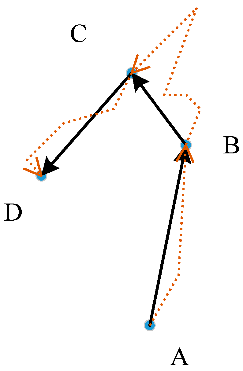
Home range (HR) estimation is a central topic in spatial ecology studies and is fundamental to understanding animal behavior [1,2,3]. An HR was originally defined as the area inhabited by an animal or group of animals in which an animal acquires resources, mates, reproduces, and takes care of its offspring [3]. Fleming et al. defined the HR area as a percent coverage of the region encompassing the probability distribution of all possible locations [4]. A large number of complex factors influence the locations and sizes of animal HRs [5,6,7], such as the behavioral characteristics of animals, the geographical environment, body size and group size; therefore, estimating the extent of an HR is still challenging in the ecological domain [7]. Powell [8] noted that “A HR estimator should delimit where an animal can be found with some level of predictability, and it should quantify the animal’s probability of being in different places or the importance of different places to the animal.” Getz and Wilmers [1] noted that an HR is subject to two types of statistical errors: type I (excluding valid areas) and type II (including invalid areas) errors. Chirima and Owen-Smith [9] introduced several criteria to assess the performance of alternative HR estimation methods. These criteria are as follows: (1) ability to naturally represent the probability or possibility of the distribution of an animal; (2) ability to bypass obstacles such as cliffs, mountains, rivers and roads for some types of animals; (3) ability to consider the impact of the terrain; and (4) minimal bias in the size of the HR. The criteria 2 means that an animal cannot live in or cross some geographic objects; for example, a deer cannot live in water or cross a deep river. Criterion 3 indicates that different topographic features have different effects on animal activities; for example, deer prefer relatively flat marginal areas of forest to rough areas. These two criteria indicate that animal activities are anisotropic. In addition to these criteria, two new requirements must also be considered. The first requirement is that a HR should include some areas with some non-zero possibility of animal activation and the second is that type I error be reduced as much as possible. Currently, global positioning system (GPS) transmitters are commonly used to track the locations of animals [3], and the transmitter will return location data for animals at certain time intervals. At the hourly scale, animals rarely walk in a straight line. Therefore, there is some non-zero possibility that an animal walked along the red line, which may be part of the home range of this animal (Figure 1).
1.1. Previous Work
One of the oldest and simplest estimators may be the minimum convex polygon (MCP), which calculates the HR extent by drawing a convex polygon around the location points of an individual. Although MCP has limitations, it is still widely applied [10,11]. Downs and Horner [12] used the characteristic hull polygons (CHPs) as a new method of home range estimation to overcome the deficiencies of MCP. This method, however, does not explicitly reveal high- and low-density use areas or clusters of points in cores [1].
Kernel density-based estimators (KDEs) [13], including fixed-kernel and adaptive-kernel methods, can express the probability of the natural HR distribution of an animal or animal group. However, KDEs suffer from difficulties in determining a suitable bandwidth and overestimating the HR [1,5,14]. In addition, traditional KDEs are based on the Euclidean distance, and the influence of terrain and obstacles on the distance between objects in space is difficult to consider. In other words, these methods struggle to account for the anisotropy of animal activities.
The local convex hulls (LoCoH) method [15] has three variants: k-LoCoH (fixed number of neighbors), r-LoCoH (certain radius r of each reference point) and a-LoCoH (all points within a variable sphere around a reference point, such that the sum of the distances between these points and the reference point is less than or equal to a). One assumption of the MCP and LoCoH methods is that the location of an animal has no error, but this condition is impossible in the real world. Another issue is that LoCoH methods yield a sharp boundary for the core area or HR; however, the HR of animals usually has fuzzy boundaries, and it is not sharp in some location of boundaries of the core area or HR. However, Getz and Wilmers [15] claimed that LoCoH methods perform much better than kernel methods in fitting utilization distributions (UDs) to HRs with distinct boundaries determined by geographic or physiographic features such as cliffs and rivers. These methods were better than the α-hull methods at incorporating all points into the HR. However, when obstacles exist or the terrain of the active region is uneven, the methods mentioned above have limitations.
In recent years, some estimators have been developed to overcome the limitations of the abovementioned estimators, and these estimators include the Brownian-bridge method (BB) [16,17] and the potential path area (PPA) approach (Long et al., 2012) [18]. However, these methods model the occurrence distribution, which does not quantify the HR, but instead, estimates where an animal is located during an observation period [4]. These types of methods are beyond the scope of this study. Additionally, some estimators have addressed the problem of obstacles [19,20,21]; for example, Long addressed the problem using the cost surface produced based on the slope [19]. However, the costs of uphill and downhill gradients are often different for animal activities, leading to cost surfaces produced by the slope alone being insufficient for HR estimation.
1.2. Purpose and Organization
As previously discussed, existing methods have both advantages and shortcomings. When obstacles and terrain are taken into account, the anisotropic perspective should be introduced into HR estimations [19], because the movements of animals are directional, leading to anisotropic locations. We propose a novel HR estimator based on fuzzy set theory [22,23,24] because the HR is a typical fuzzy phenomenon, namely, the density-based fuzzy home range estimator (DFHRE), which integrates the advantages of active learning methods (ALMs) [25]. The remainder of this paper is organized as follows. In Section 2, two datasets are introduced. Section 3 provides the methodology. In Section 4, the results are presented, and we discuss the DFHRE and the other estimators. Section 5 presents the conclusion.
2. Materials
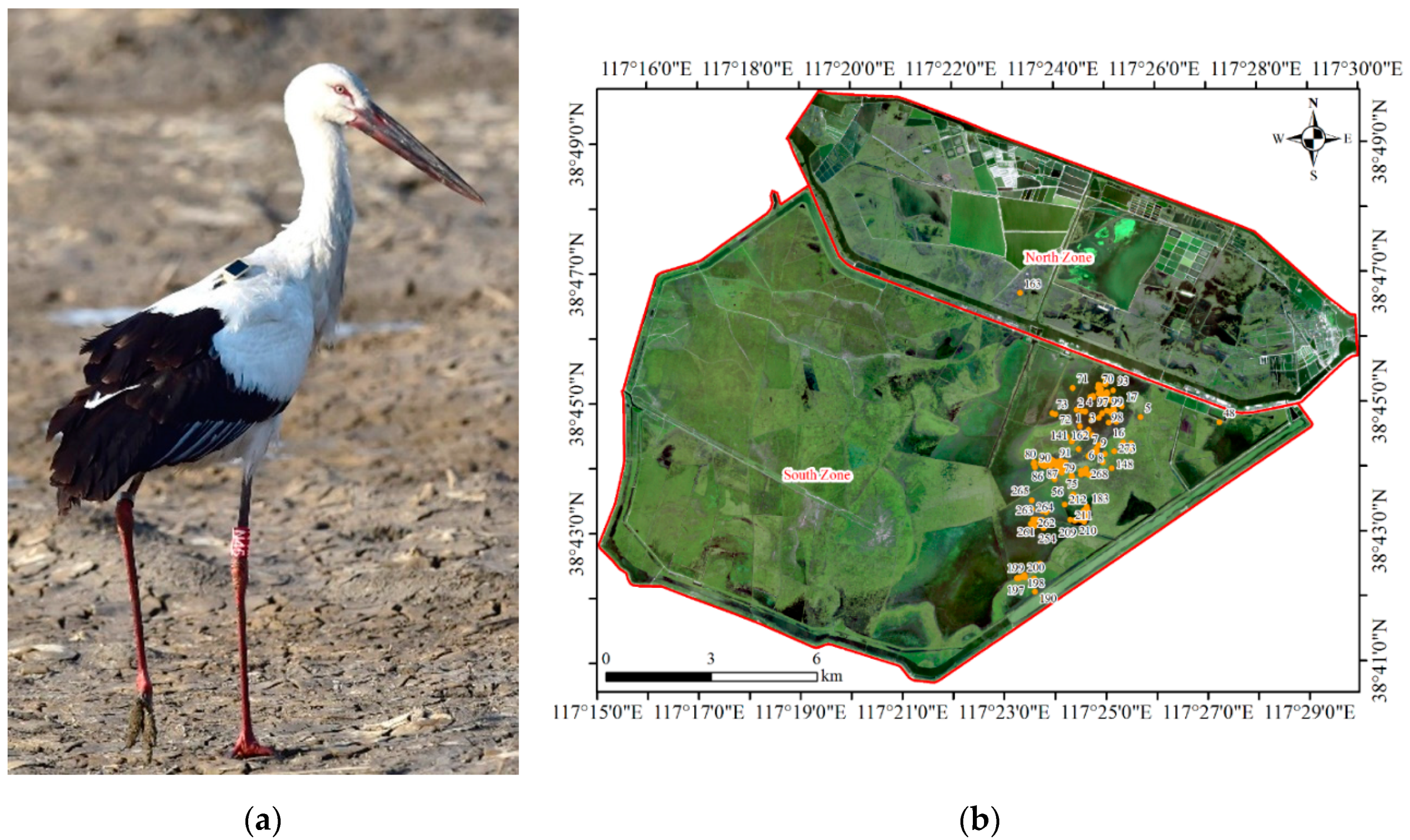
Two datasets are used to verify the methods proposed in this study. The first dataset was acquired by a GPS locator attached to a rescued oriental white stork (Ciconia boyciana), which was rescued by our school’s migratory bird rescue team in the spring of 2016. The error of the GPS locator was 5 m. The oriental white stork is a large wading bird that often forages in swamp, wetland, and pond waters, mainly eating fish, frogs and insects. The distribution of oriental white stork breeding was mainly concentrated in the Russian Far East and Northeast China, and wintering areas were concentrated in the Yangtze River Basin, China. The oriental white stork arrives at its breeding ground in March every year and begins to leave from late September to early October. The Beidagang Reservoir is a natural reservoir for migratory birds and an important migratory stopping point for oriental white storks. The reservoir is located in the Tianjin Binhai New Area at a latitude of 38°41´ to 38°50´ E and a longitude of 117°15´ to 117°15´ N, as shown in Figure 2.
The locator sends the coordinates of the bird to the receiver every hour, and the movement trajectory of the bird is recorded. In the spring, this bird mainly lived in the south zone (Figure 2). Two distinct outliers (ID = 48 and ID = 163) were deleted, and 271 points were ultimately obtained.
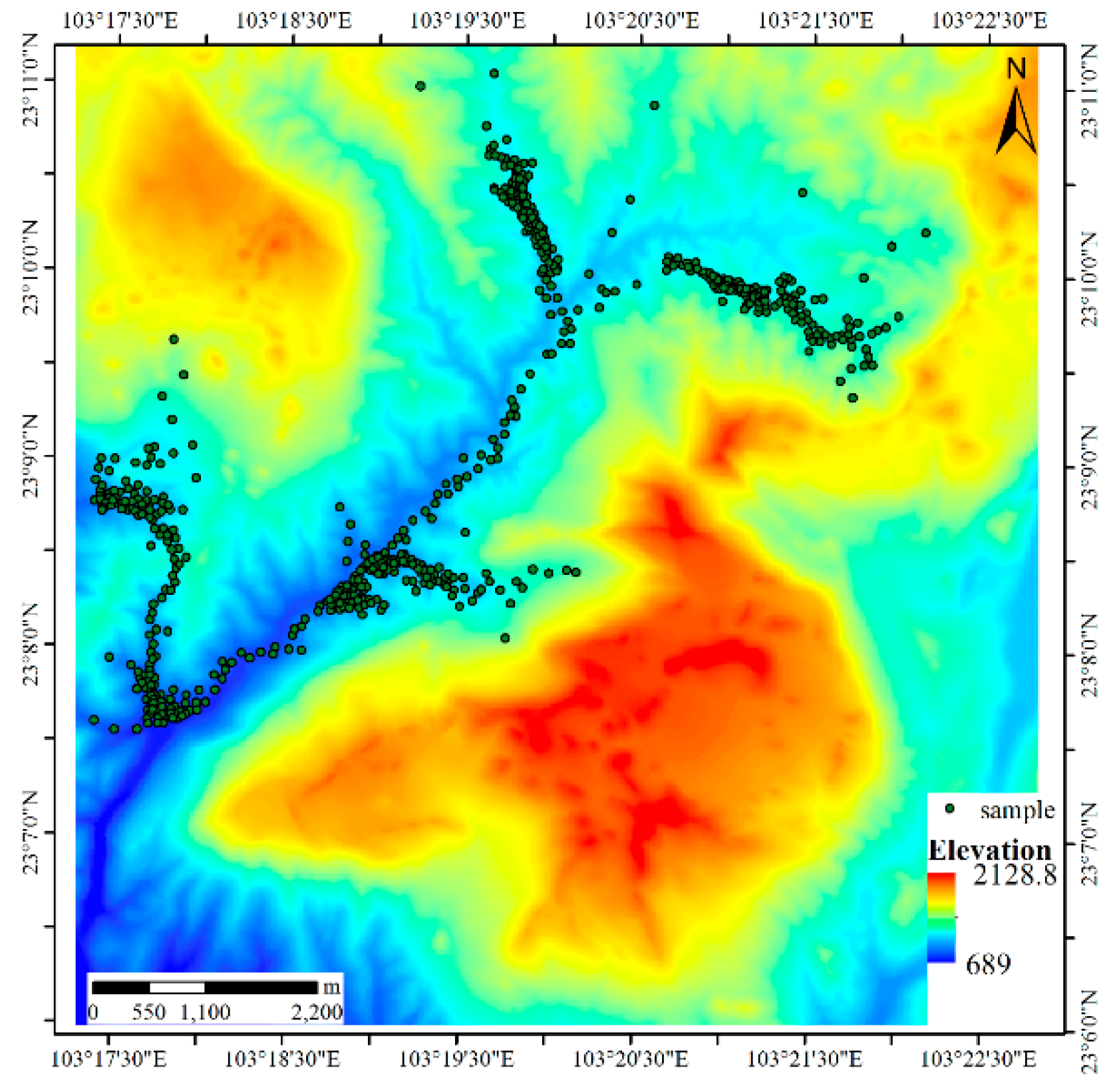
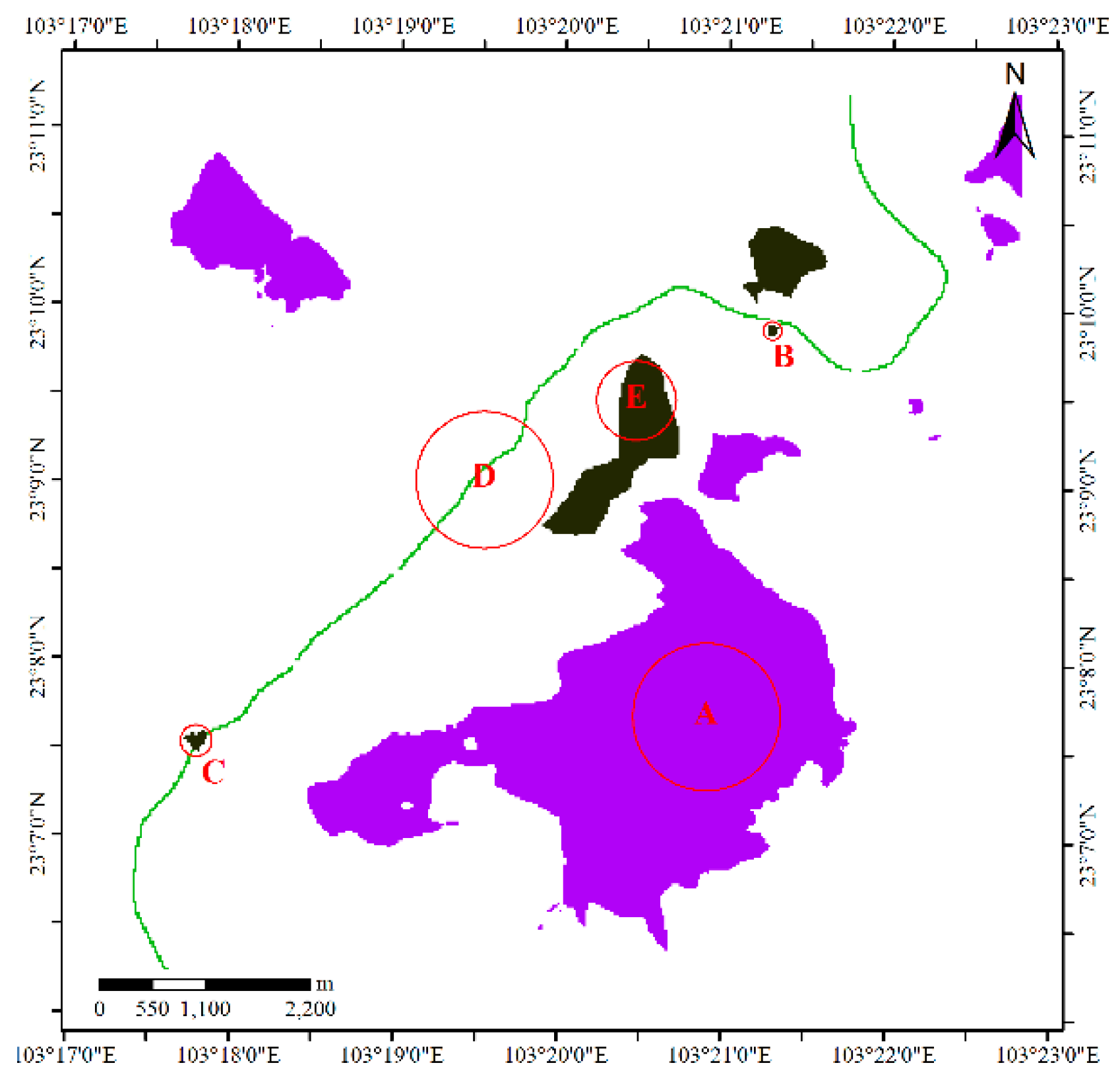
The second dataset (Figure 3) is a simulated dataset about sika deer (Cervus nippon), which like to live on the edges of forest and grassland areas but not in dense forests or thickets; additionally, they prefer regions with little human disturbance and abundant open spaces and water sources [26,27]. According to these habits, we use a digital elevation model (DEM) and remote sensing image to select sample points manually. We concentrated the sample points in the valley and edge areas of a forested region, and obstacles such as highways, farmlands, water bodies and villages were avoided when choosing sites. The DEM data were provided by the National Geomatics Center of China at a spatial resolution of 25 m. The elevation in this region is between 689 m and 2129 m. In this study, regions with elevations higher than 1800 m (labeled A in Figure 4), pools (B in Figure 4), expressway service areas (C in Figure 4), expressways (D in Figure 4), and farms (E in Figure 4) were considered obstacles to sika deer activities (Figure 4). Because the animals prefer to live on flat terrain rather than in rugged and steep areas, the height differences derived from the DEM are used to measure the cost distance in this region.
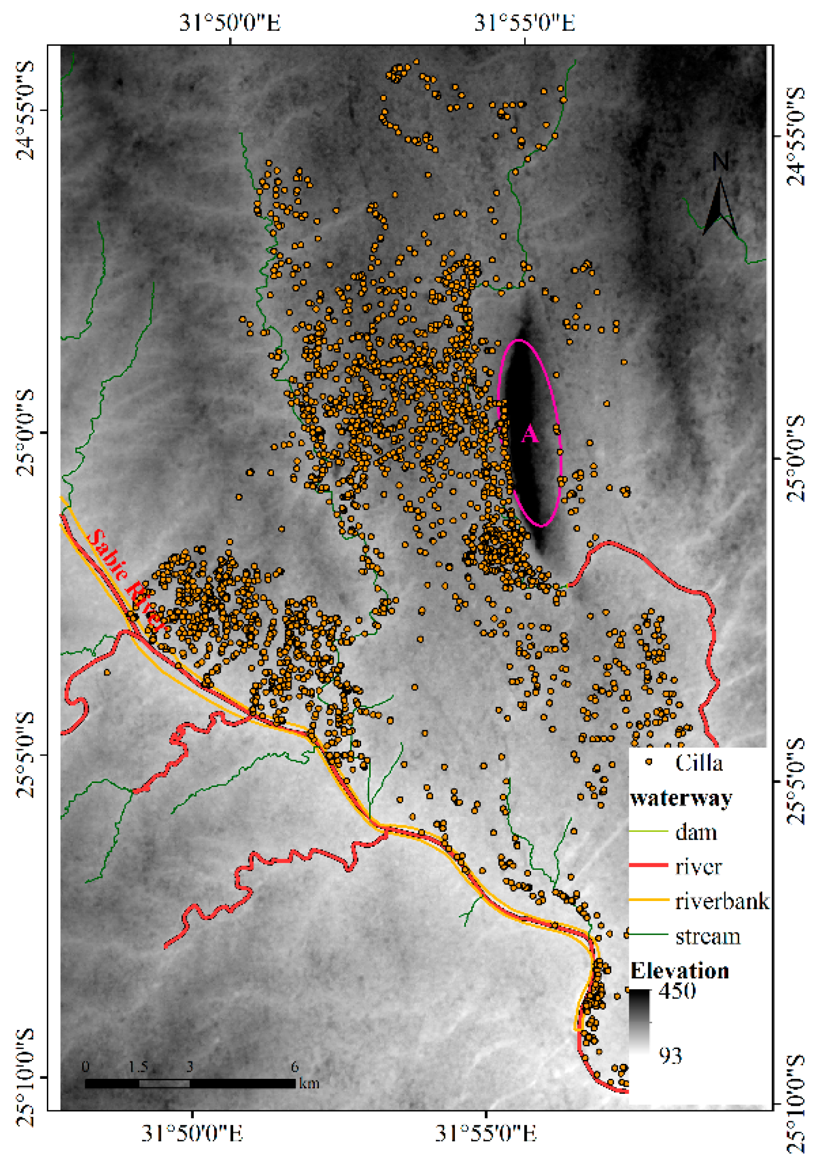
The third dataset is the tracked data for Cilla, an individual African buffalo [15,28] that was tracked at the Lower Sabie region of the Kruger National Park for 147 days between July and December 2005, yielding 3528 location points. The DEM was downloaded from the Geospatial Data Cloud (http://www.gscloud.cn/), and its spatial resolution is 30 m. The waterway layer was obtained from the OpenStreetMap (https://www.openstreetmap.org). Almost all the points are on the east side of the Sabie River, so in this experiment, the Sabie River is an obstacle to Cilla’s activities, and the nearby mountains (Labeled A in Figure 5) also restrict activities.
3. Methods
In this section, we introduce a new HR estimator, based on the ALM. To consider the anisotropy of animal monitoring points, the cost distance based on geodesic distance transformation is used as a distance measurement between points.
3.1. Framework of the DFHRE
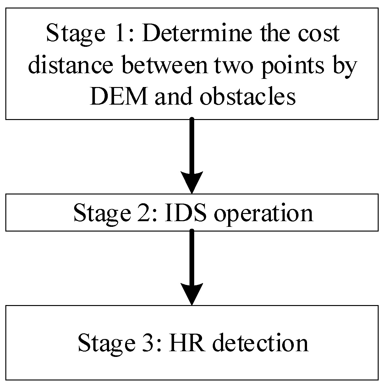
The framework of the proposed DFHRE is composed of four stages (Figure 6). The DFHRE is operated in raster space, so all data should be digitalized in raster format. The resolution of the raster is important for subsequent analysis. These three datasets introduced in Section 2 correspond to three different experiments. As a result, the resolution of the first dataset is set to 20 m, which is consistent with the resolution of the remote sensing data used in subsequent research, and the resolutions of dataset 2 and dataset 3 are set to 25 m and 30 m, respectively, which are consistent with the resolution of the DEM.
3.2. Determining the Cost Distance
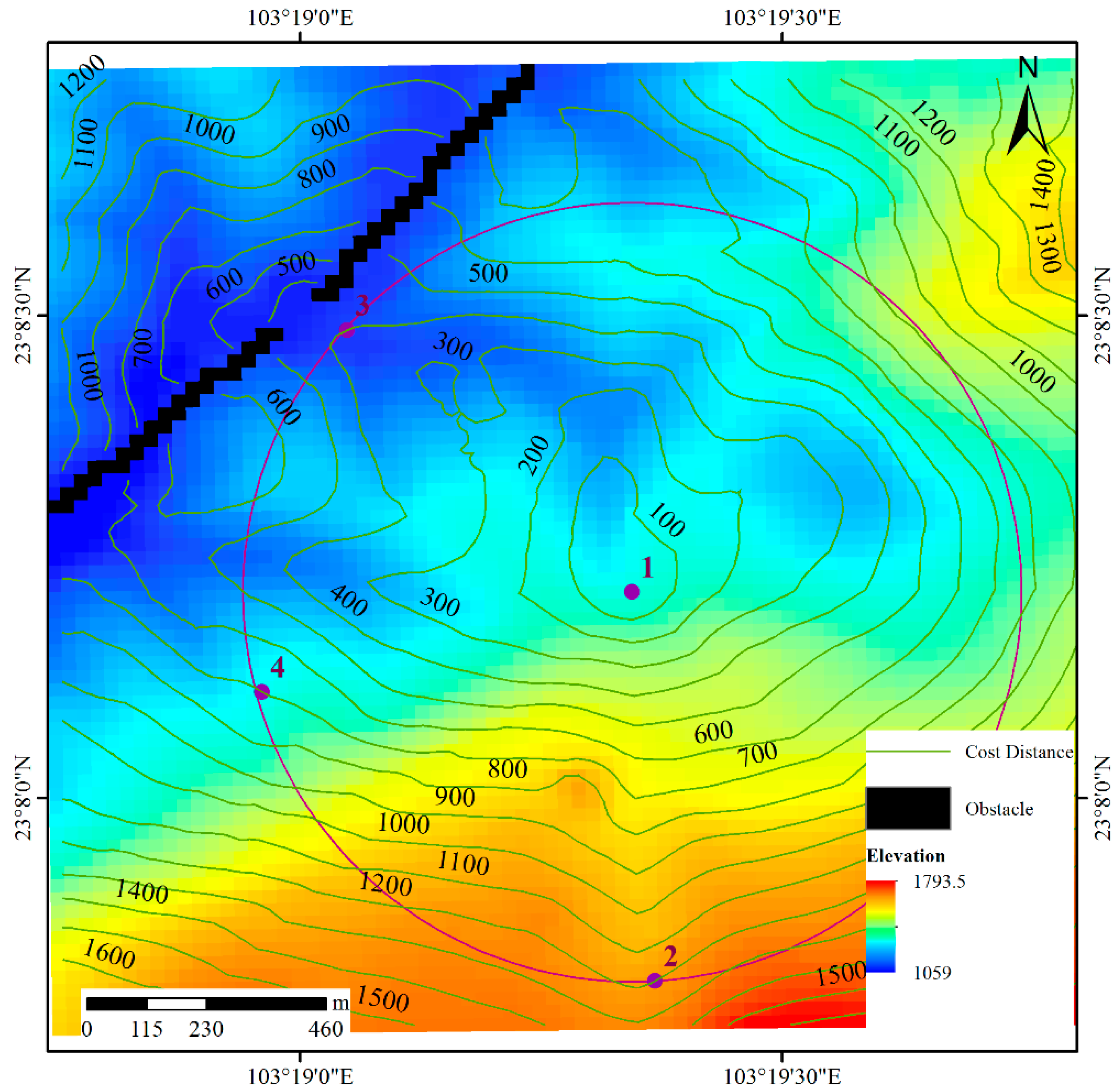
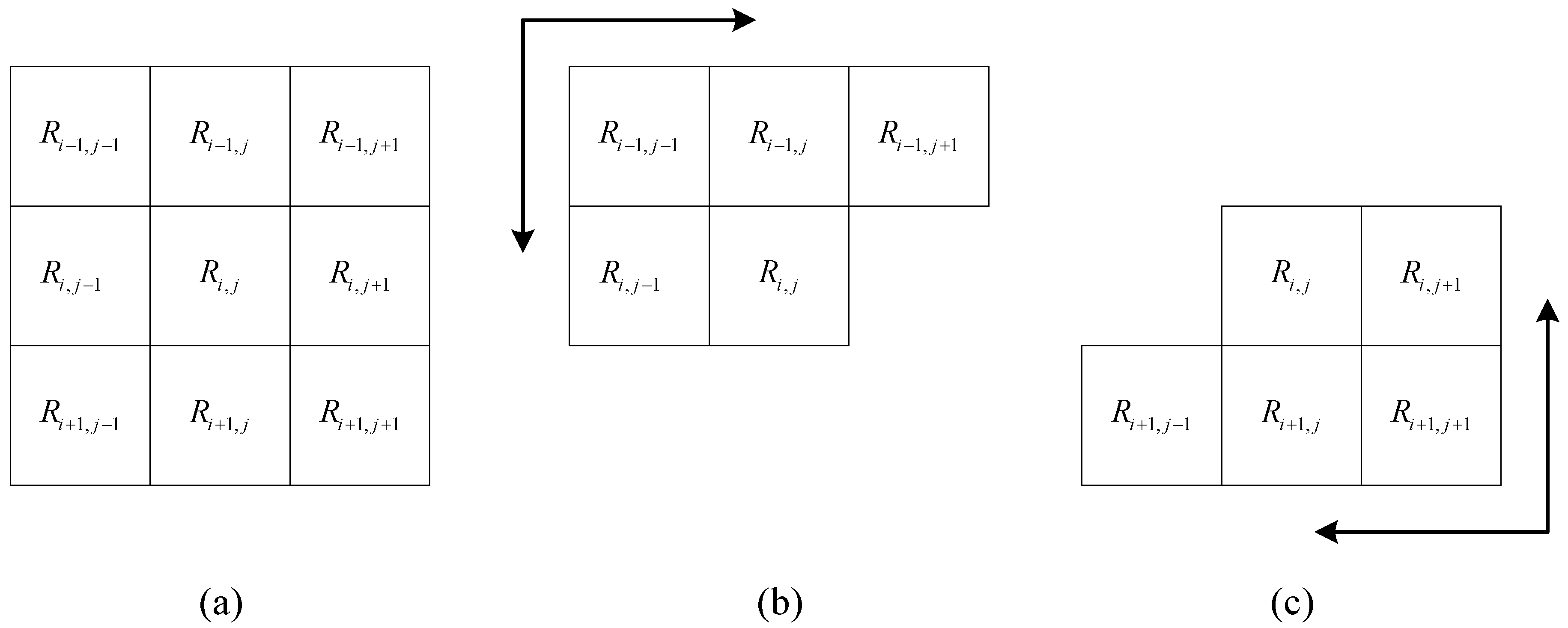
Sample points can be anisotropic when obstacles and terrain are considered in natural environments. For example, point 1 in Figure 7 is a source point; the center of the purple circle is at point 1, and the radius is 700 m. As a result, the Euclidean distances from point 1 to points 2, 3 and 4 are equal. However, the elevation increases from point 1 to point 2 and decreases from point 1 to point 3, and the elevation of point 1 is similar to that of point 4; thus, it is intuitively believed that it is easier to move from point 1 to 3 than from point 1 to 2 and from point 1 to 4. Considering the anisotropy of animal movements, the cost distance induced by least-cost modelling and the map algebra-distance transformation with obstacles (MA-DTO) algorithm [29] are adopted in this study. This algorithm is implemented in raster space and based on the structure of eight neighbors (Figure 8a). Let the image size be M × N, and the size of the neighbor window be 3 × 3. Then, the height difference between a cell in this image (relief amplitude) and one of its neighbors in Figure 8a is expressed as follows:
where is any cell in the DEM, is any neighbor of , and and are the elevations of points and , respectively. Then, the cost distance of the original point to any point in space can be calculated in terms of the following three steps.
- Step 1: Let the image size be M × N. The distance matrix D(M × N) is used to express the distance of any point to the original point, and the initial distance is set to a very large value, such as the maximum value of the integer type. If point (m, n) is the original point, set D(m, n) is equal to 0.
- Step 2: Scan matrix D from the upper left corner to the lower right corner, where i = 0, 1, 2, …, M–1 and j = 0, 1, 2, …, N–1, as shown in Figure 8b. The distance matrix D is updated by:where S is the resolution of the raster data and k is the parameter used to adjust the movement difficulty. If is an obstacle, no further steps are required.
- Step 3: Scan matrix D from the lower right corner to the upper left corner, where i = M–1, M–2, …, 0 and j = N–1, N–2, …, 0, as shown in Figure 8c. The distance matrix D is updated as follows.If is an obstacle, no further steps are required.
Through steps 2 and 3, we can obtain the cost distance from any point to the source point in the raster space. In Figure 7, the green lines represent the cost distance to point 1. It is clear that although the Euclidean distances between points 1 and 2, 1 and 4, and 1 and 3 are equal, the cost distance from point 1 to 2 is larger than that from point 1 to 4 and from point 1 to 3. The reason for this difference is that the elevation of point 2 is higher than that of points 3 and 4. If there are obstacles between one point and the original point, the movement of animals will bypass these obstacles, as shown in Figure 7. Generally, the value of k depends on the living habits and environment of animals. Notably, if the terrain is flat, the influence of the terrain factor should not be considered; in this situation, k is set to 0. Additionally, different animal species have different climbing abilities; for example, tigers, goats, and horses have different climbing abilities. Tigers like to live in mountainous areas, and horses like to live in flat regions. Therefore, a rough and simple approach to determining k is the method of ranking the climbing ability of different animals; in this solution, k can be a static value. A more detailed approach is the resource selection method [30,31]. In this method, the resource selection probability function (RSPF) gives the probability that a particular resource, as characterized by a combination of environmental variables, will be used by an individual animal. Horne et al. [31] adopted this approach and proposed a synoptic model s(x) of animal space use as a function describing the probability density of environmental covariates. In this study, s(x) is adopted to determine the value of k for different relief amplitude values. Because we concentrate on the influence of different relief amplitude values on HR, there is one covariate in s(x), and it is a function of the relief amplitude. Thus, s(x) is expressed as follows:
where is the relief amplitude at location x and is the Gaussian density function of the relief amplitude. The larger the value of s(x) is, the higher the preference degree of animals for a relief amplitude value, and vice versa. The influencing coefficient of relief amplitude on distance is expressed as follows:
3.3. Determining the Possibility Distribution with IDS Operations
Usually, the probability theory offers a good quantitative model for randomness and indecisiveness, and possibility theory offers a good qualitative model of partial ignorance [24]. As a classical measure of possibility [22,23], the fuzzy set uses the membership value to describe the possibility of an object belonging to a set, with the range of membership values being [0,1]. Usually, Gaussian, triangular and trapezoid membership functions are used to describe the fuzziness of the attributes of an object in practice.
The ink drop spread (IDS) operator is the core of ALMs and acts as a fuzzification operator. ALMs have been successfully used for function approximation [32] and classification [33]. First, the possibility distribution is estimated by the IDS operator; then the membership degree of the HR, which indicates the importance of different places to an animal, is produced. To improve the IDS operation and consider the terrain and obstacles, the cost distance [34,35] is used to replace the Euclidean distance. The classical IDS operator assumes that each data point is isotropic, meaning that the ink drops extend to the surroundings, and when the ink drops overlap, some regions become increasingly dark and form arbitrarily shaped ink patterns. Moreover, this operator assumes that the surface should be planar and contain no obstacles. However, a real surface is often inclined, and ink drops should spread in the direction of downward inclination in this case. When obstacles are encountered during the spreading process, the ink drops will bypass the obstacles. In addition, the activities of animals are very different from those of water droplets. Animals can go uphill and downhill. In addition, it is comparatively easy for animals to go downhill and more difficult for them to climb than move on flat land. As a result, animal movements are anisotropic, which should be considered, and the cost distance is used to replace the Euclidean distance in this stage.
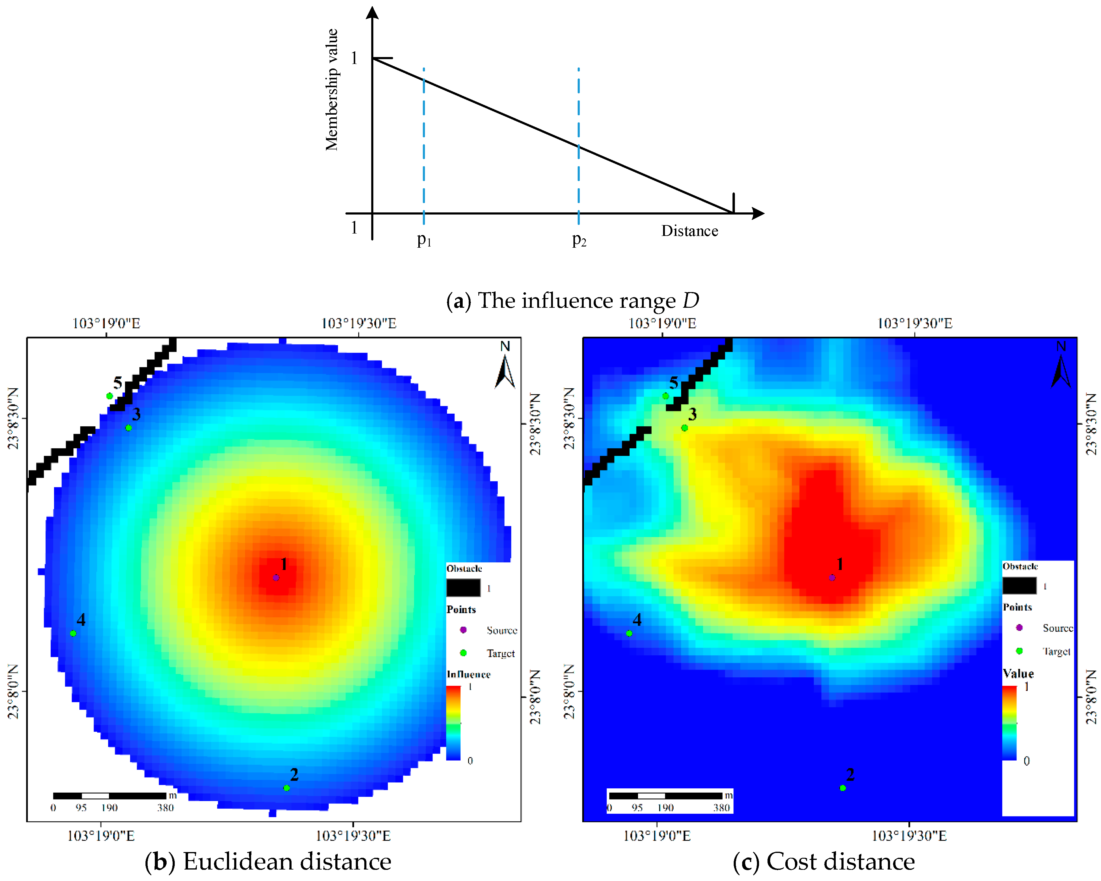
In classical ALMs, an ink drop spreads isotopically in the IDS plane when considering the degree of uncertainty in the vicinity of a data point [33]. The influence area of adjacent points or the uncertainty regions around these points may overlap. In this study, the triangular fuzzy number is used to express the influence range D (Figure 9a) of sample points and is expressed as follows:
where d is the distance from a target point to a source point and D is the influence range of a source point. The membership value of a point describes the influence degree of a sample point on this point; thus, the larger the influence degree is, the larger the possibility of this point belonging to the HR. For example, the influence degree of p1 is larger than that of p2, and p1 has a larger possibility of belonging to the HR than does p2. Here, the influence range D is the maximum radius of movement of animals in a given period of time under normal conditions. The ad hoc smoothing method is a useful way to determine the value of D, and we will discuss this approach later in the paper.
The influence area of a sample point can be determined by Equation (6). Assuming that D is 800 m, the Figure 9b shows the influence area of a source point when the Euclidean distance is used in a classical ALM. Target points 2, 3, and 4 have the same influence on the source point because these three points have the same Euclidean distance to the source point. Target point 5 is not influenced by the source point because the Euclidean distance from point 5 to the source point is larger than the value of D. The influence area of the source point is shown in Figure 9c when the Euclidean distance is replaced by the cost distance (Section 3.2); although points 2, 3 and 4 have the same Euclidean distance to the source point, their cost distances are clearly different. We can see that target points 3 and 4 have a different influence degree of the source point. Point 2 is not influenced by the source point because the cost distance from it to the source is larger than D, and the influence value at point 5 is 0.32 because the cost distance from it to the source is less than D. Therefore, the difference between the cost distances from points 2, 3 and 4 to the source point leads to different influence degrees, and with this approach, the anisotropy of animal activity is described.
If a cell in the IDS plane is influenced by several source points, it is necessary to overlap all of the ink patterns of these source points. Usually, the overlap of all ink patterns can be modeled by sum operators, and the full IDS plane can be filled by the ink patterns that describe the influence degree of all sample points. Let H be the influence area of sample t, which is converted from the cost surface by Equation (6); then, the full IDS plane is expressed as follows:
where T is the number of source points. The is the influence degree of source point t on cell (i, j), as shown in Figure 9. Then, the full IDS plane is normalized to the range of (0,1), and the possibility distribution function (PDF) or the membership grade of the HR can be determined. In this study, the proposed method assumes that data are independent and identically distributed (IID).
3.4. Detecting Core Areas and HRs
3.5. Determining the Initial Parameters
Two parameters are crucial for the DFHRE. We adopt the resource selection method to optimize the topographic influence parameter k. The influence range D is very similar to the bandwidth of the kernel density estimators, so we can adopt the identification method of the bandwidth to select an appropriate D. There are some automated methods that can be used to select an appropriate bandwidth. The reference method () assumes a normally distributed dataset, but generally performs poorly, except for applications involving unimodal distributed datasets [38]. The least-squares cross validation (LSCV) method () is widely used in related studies, but it has a tendency to select low bandwidth values that produce fragmented UDs [39,40] and numerical limitations of points [41]. The ad hoc smoothing method () was designed to prevent over- or under-smoothing, and this method involves choosing the smallest increment of that results in a contiguous 95% kernel HR polygon that contains no lacuna [42]. This technique is repeatable and defensible given that the proper biological questions are posed prior to analysis [40]. In this study, we adopt the ad hoc smoothing method to select the appropriate D. It should be noted that when k in Equations (2) and (3) is equal to 0 and no obstacle is taken into account, the cost distance is simplified to the Euclidean distance and D is reduced to an ordinary bandwidth.
3.6. Implementation in Java
The algorithm described in this section is implemented in Java, and the open-source package Geotools [43] is used. At first, all sample points are digitalized as a raster layer. For the second experiment, the DEM is needed, and the obstacle data are processed in ArcMap. For each sample point, the cost surface from this sample to any location in space is calculated by Equations (1)–(3). In calculating the parameter k, the relief amplitude is calculated from the DEM, and the Gaussian density function of the relief amplitude can be obtained. Then, the influencing coefficient of relief amplitude k is calculated from Equations (4) and (5). The influence area of each sample can be produced by Equation (6), and the PDF of the HR is obtained from Equation (7).
4. Results and Discussion
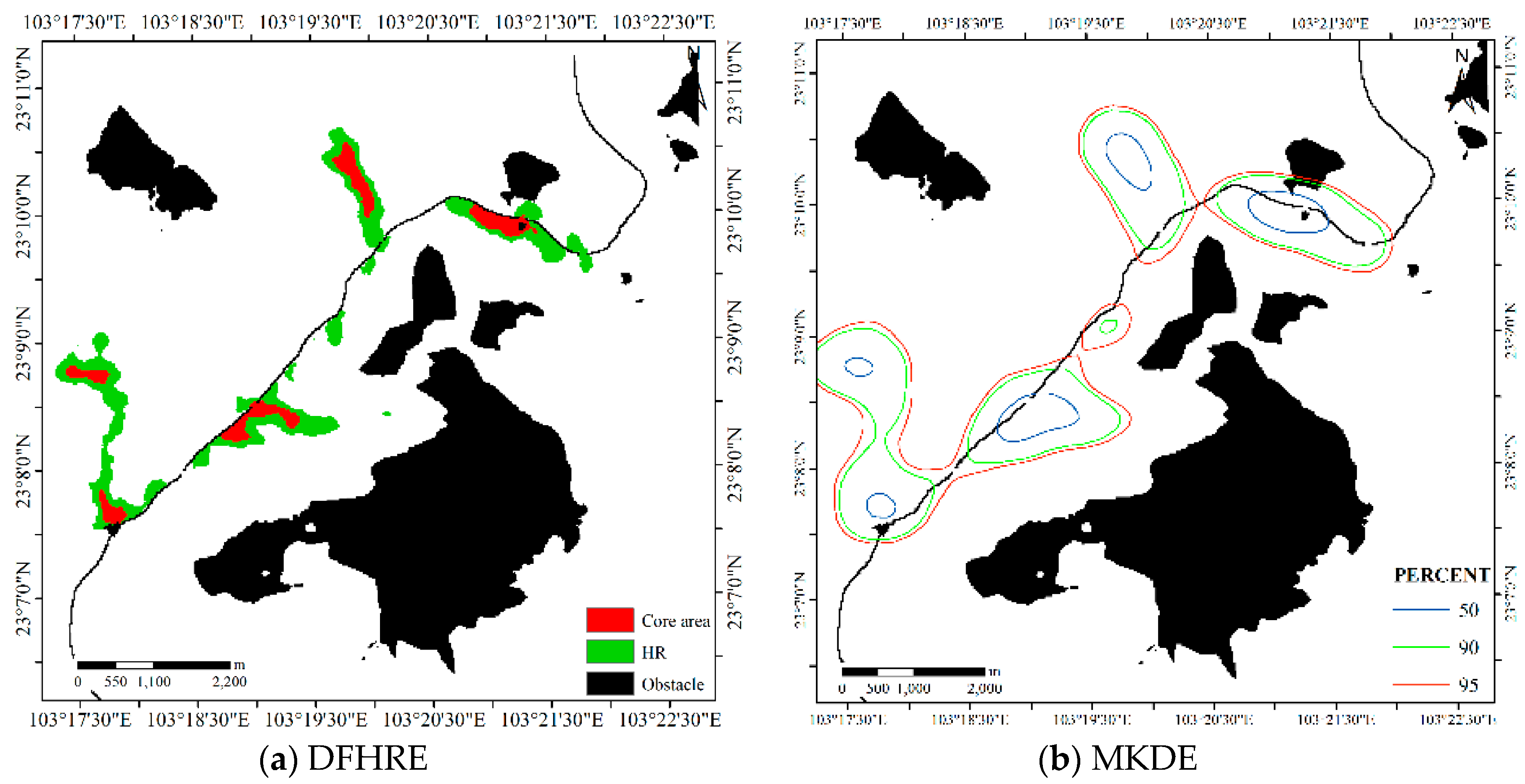
Because the Beidagang Reservoir is very flat and there are no obstacles in this reservoir that can interfere with the activities of the oriental white stork, the effects of terrain and obstacles are not taken into account. The sample layer is digitalized into a raster layer with a resolution of 20 m, and the Euclidean distance is used, which means that k = 0 in Equations (2) and (3). D is set to 421 m with the ad hoc smoothing method.
For the Dataset 2, as described in Section 2, five types of obstacles are taken into account. The cost distance layer of each sample is calculated by Equations (1)–(3) with the DEM and obstacle layer, and the value of k for different height differences in Equations (2) and (3) is determined by Equations (4) and (5). The best choice of D is 278 m according to the ad hoc smoothing method.
Similarly, the best choice of D for Dataset 3 is 840 m based on the ad hoc smoothing method, and the value of k is determined by Equations (4) and (5).
4.1. Results
4.1.1. Results for Dataset 1
4.1.2. Results for Dataset 2
4.1.3. Results for Dataset 3
4.2. Analysis of the DFHRE
The characteristics of the DFHRE can be summarized as follows.
(1) The DFHRE can consider the undulating terrain and bypass the obstacles via a geodesic distance transformation with the DEM and obstacles. The Euclidean distance will be used if the terrain and obstacles are not considered.
(2) The DFHRE uses a membership grade to express the gradual change in the possibility degree of any location belonging to a HR; thus, it is suitable to express the fuzzy scope of the HR.
4.3. Comparisons with Other Estimators
To verify the effectiveness of the proposed method, we compare it with two popular methods: KDE and LoCoH. The multivariate kernel density estimation (MKDE) based on the plug-in selector [40,41] is an effective fixed-kernel method, and it is used in this section; the adaptive kernel method in KDE is implemented by the Home Range Tools package for ArcGIS® 10.x (HRT 2.0) [42]. While the LoCoH is implemented with the HR Analysis and Estimation (HoRAE) toolbox [38]. As previously mentioned, the MCP method results in extensive overestimation; thus, we will not compare it with the presented method. Specifically, the MKDE and adaptive kernel methods in KDE and the r-LoCoH and k-LoCoH methods are compared.
4.3.1. Comparison for Dataset 1
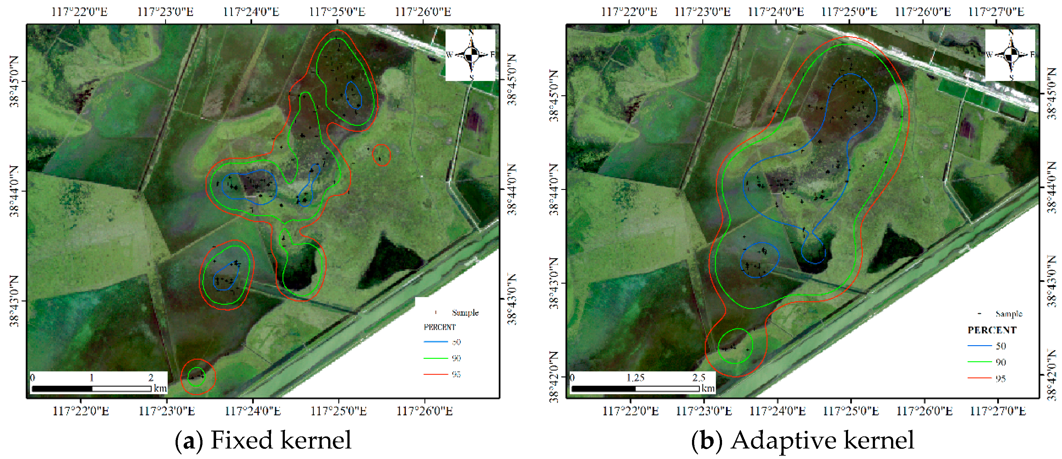
For the MKDE, the bandwidth matrix is determined by the multistage plug-in bandwidth selector as ; the adaptive kernel method is an automated method that uses a different bandwidth for each data point [13], and the estimated results are shown in Figure 13. Two core areas are produced by two kernel methods, and the results are relatively concentrated. Table 1 reports the sizes of the core areas and HR. From the perspective of size, the MKDE produces smaller core areas and a smaller HR than the adaptive kernel method, and the proposed DFHRE approach produces the smallest HR.
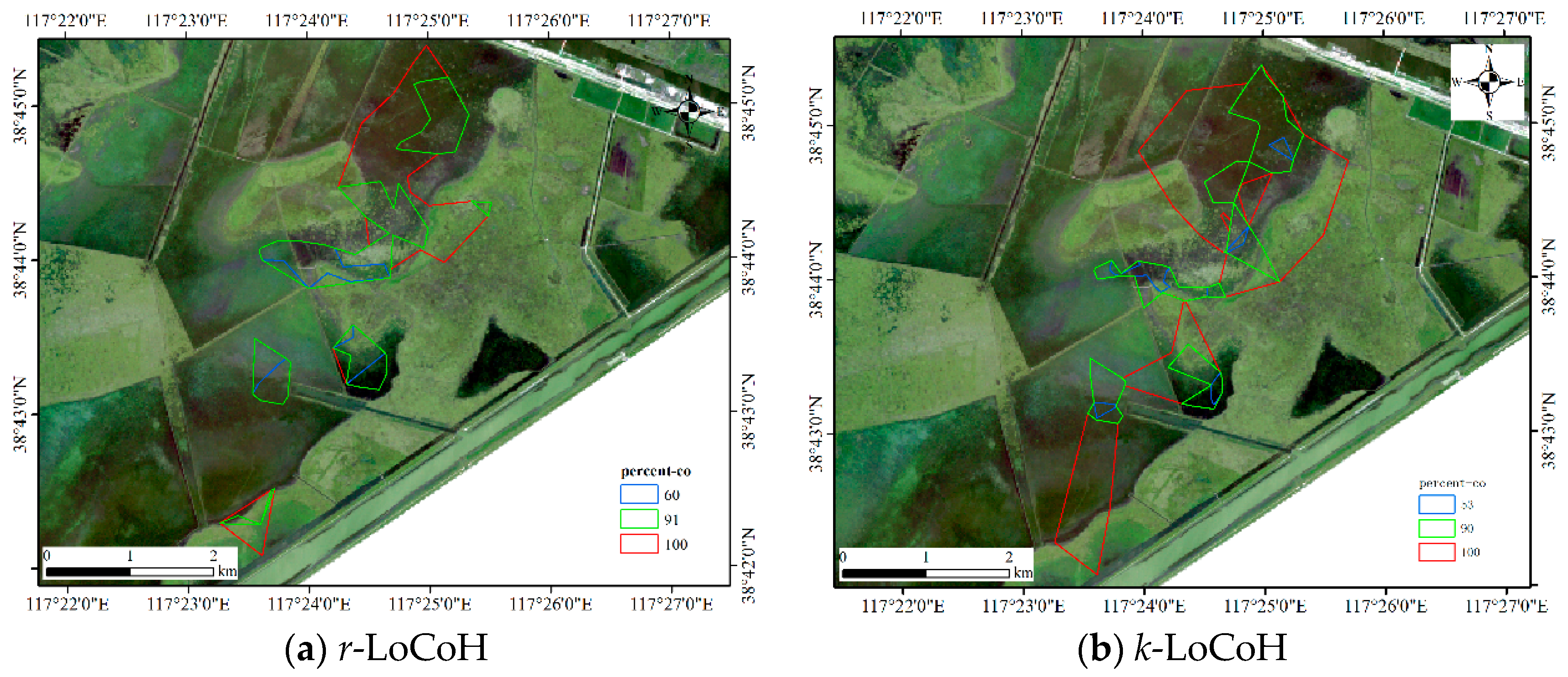
For the LoCoH method, the parameter k in k-LoCoH is determined by the recommended method (), where k = 16. The parameter r in r-LoCoH is determined by experiments and set as 500 m. The results of LoCoH are shown in Figure 14. The 60%, 91%, and 100% isopleths are achieved by r-LoCoH (Figure 14a), and the 53%, 90%, and 100% isopleths are achieved by k-LoCoH (Figure 14b). The boundaries of the core areas and HR are crisp, and at some locations, the 60%, 91%, and 100% isopleths overlap. In other words, the possibility of these locations being HRs sharply declines from 0.6 to 0, and some non-zero probability regions are excluded. Therefore, it seems very rough to express the vagueness of the HR, and the predicted HR can even be considered inconsistent with the actual situation. In contrast, the DFHRE expresses the fuzzy boundaries of HR by the possibility degree, and all non-zero possibility regions are included (KDE expresses a fuzzy boundary based on a probability), so the results of the DFHRE and KDE seem very reasonable (Figure 10 and Figure 13). From the perspective of size, the results of the LoCoH methods are shown in Table 1. Because some regions with non-zero probability are ignored by the LoCoH methods, the two LoCoH methods yield smaller areas than the DFHRE and KDE methods.
4.3.2. Comparison for Dataset 2
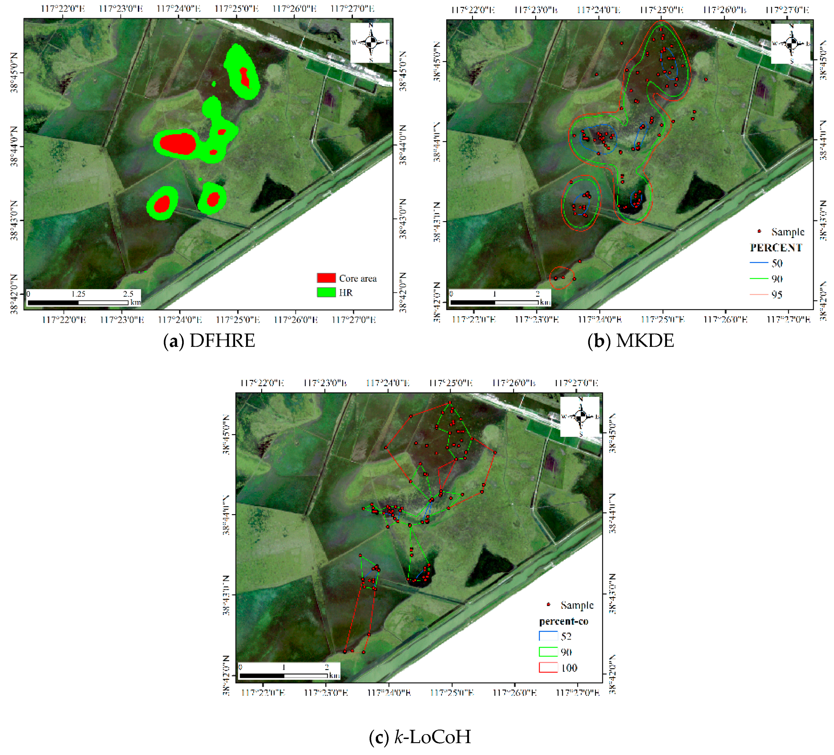
The bandwidth matrix of MKDE for this dataset is , and the bandwidth of adaptive KDE is automatically determined. The results are shown in Figure 15, and the sizes of the core areas and HR of the five methods are reported in Table 2. We can see that the MKDE and adaptive KDE results overlap with some obstacles, so they have no ability to bypass obstacles. In this study, the two KDE methods based on the Euclidean distance do not consider the effects of terrain and obstacles, so the results are inferior to those of the DFHRE. Deer like to live in valley areas, which are flatter than hillsides and suitable for deer life. In other words, mountains and obstacles will limit the sphere of activity of this type of animal. Therefore, from this perspective, the results of the DFHRE are more reasonable than those of the KDE methods. If the sizes of the core areas and HR are considered, then the core areas and HR (Table 2) are larger than those estimated by DFHRE. Therefore, for this dataset, the DFHRE is performs better than KDE.
For the LoCoH method, r = 300 m for the r-LoCoH and k = 25 for the k-LoCoH are used, and the results are shown in Figure 16. The extent of the r-LoCoH result is narrower than those of other methods. If the size of the region is concerned, k-LoCoH yields the smallest core areas but a large HR, because it covers all the samples of the dataset. The size of the 100% HR estimated by r-LoCoH is obviously smaller than that estimated by k-LoCoH because r-LoCoH removes some outliers. An obvious attribute of the result of the LoCoH method is that all boundaries corresponding to the 50%, 90% and 100% isopleths are crisp, and the latter method is used to express the degree of activity range; however, the degree of activity ranges estimated by the DFHRE and KDE exhibit gradual transitions. Therefore, from this perspective, the LoCoH method is coarser than other methods. Another default is that some regions with a non-zero probability of animal activity, as discussed in Section 1, are missing; however, the DFHRE and KDE methods can detect some regions with a non-zero possibility or probability of animal activity, and the type I error is reduced. Additionally, this method does not consider the influences of obstacles, and the HRs estimated by the LoCoH methods may overlap with obstacles, so the HRs estimated by the LoCoH methods still have defects. For example, the lake is completely covered by the HR extent, and the expressway is overlapped by the HR extent; thus, this method cannot completely circumvent the obstacles, and type II error exists. By contrast, the DFHRE method excludes all types of obstacles, and then the type II error is reduced.
4.3.3. Comparison for Dataset 3
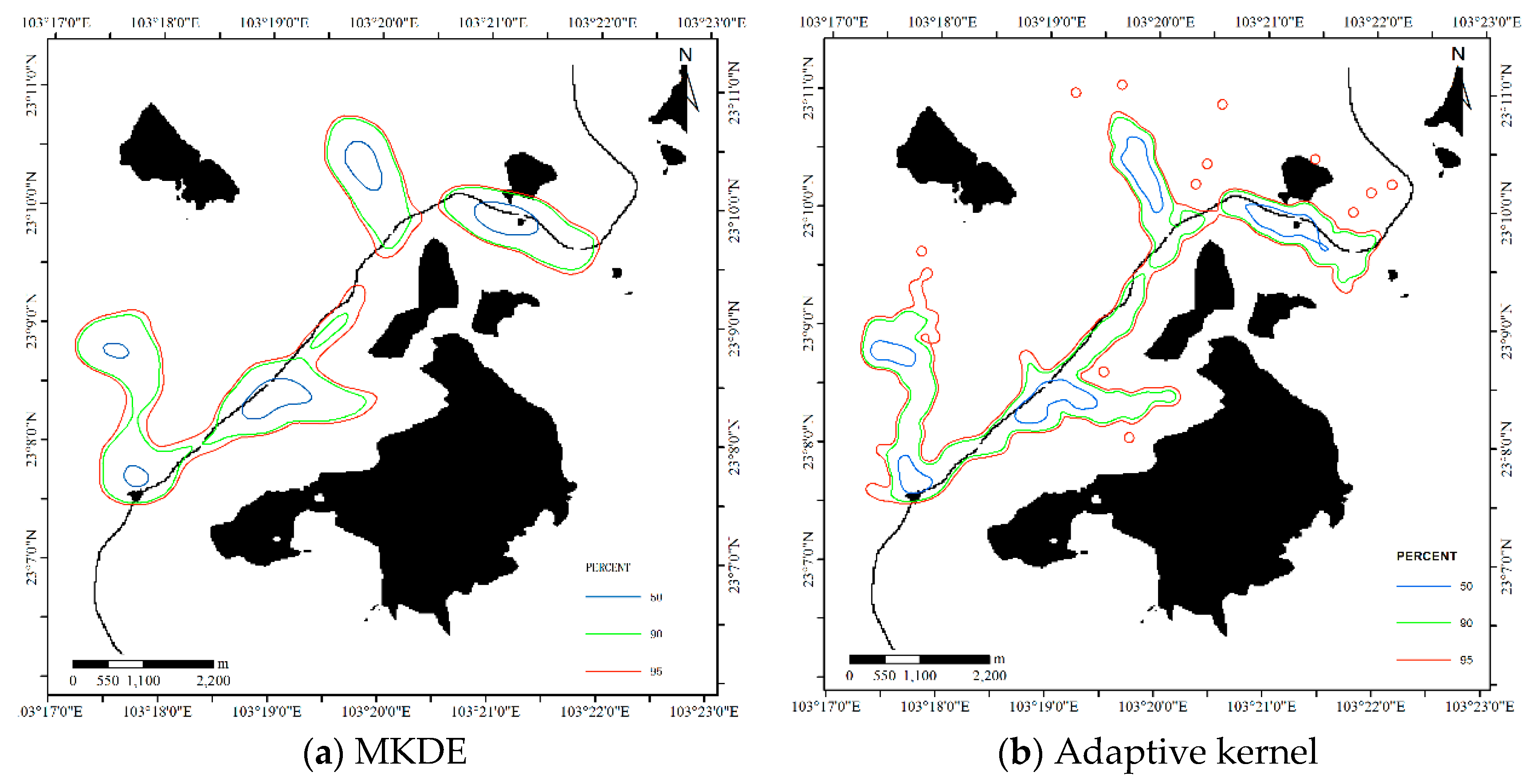
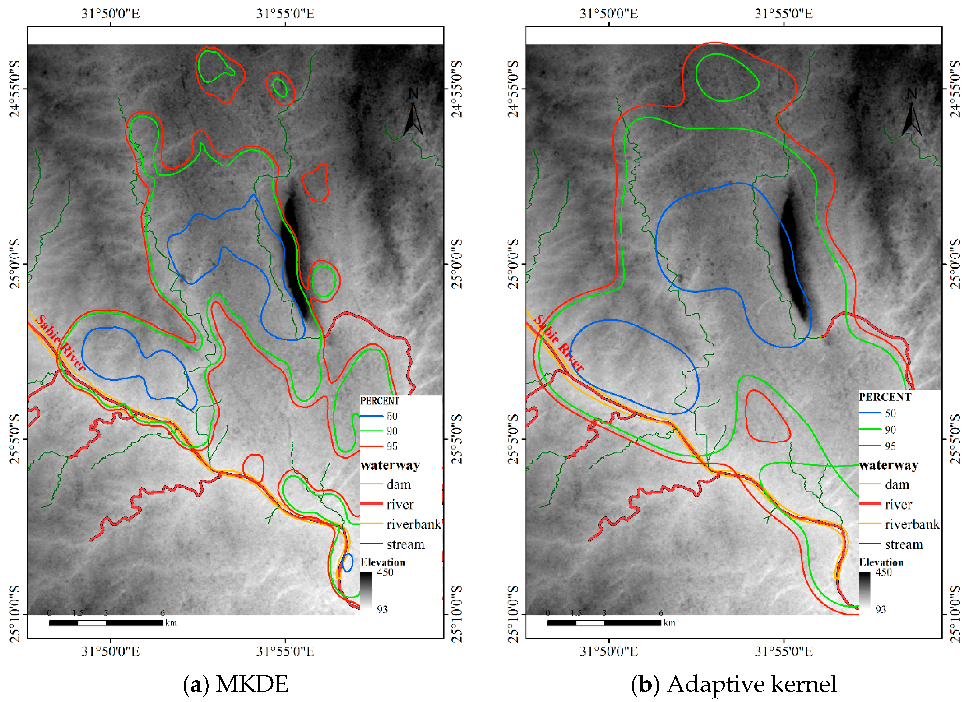
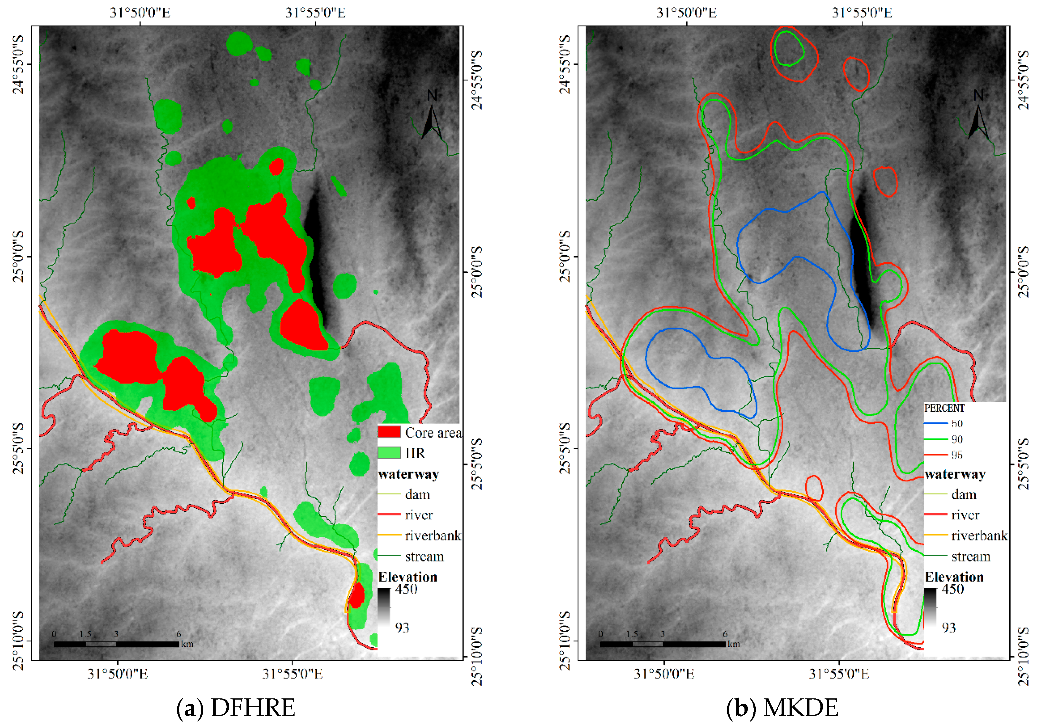
The bandwidth matrix of the MKDE for this dataset is , and the bandwidth of adaptive KDE is automatically determined. Figure 17 shows the results, and Table 3 illustrates the sizes of the core areas and HRs of the five methods. The results of the MKDE and adaptive KDE overlap with the Sabie River. Additionally, the HRs of the MKDE and adaptive KDE overlap with the mountains (Labeled in Figure 5) in a large area. However, the proposed DFHRE method based on the cost distance can consider the effects of terrain and obstacles, so the results of the DFHRE do not overlap the Sabie River but do overlap the mountains in a small area. In general, buffaloes like to live in flat areas, and deep rivers restrict their activities, but streams do not have that effect. Therefore, from this perspective, the results of the DFHRE are more reasonable than those of the KDE methods. From the point of view of area, the core areas and HRs (Table 3) of the KDE are larger than those estimated by the DFHRE, and then the result of the DFHRE has less type II error than that of the KDE. Therefore, for this dataset, the DFHRE performs better than the KDE.
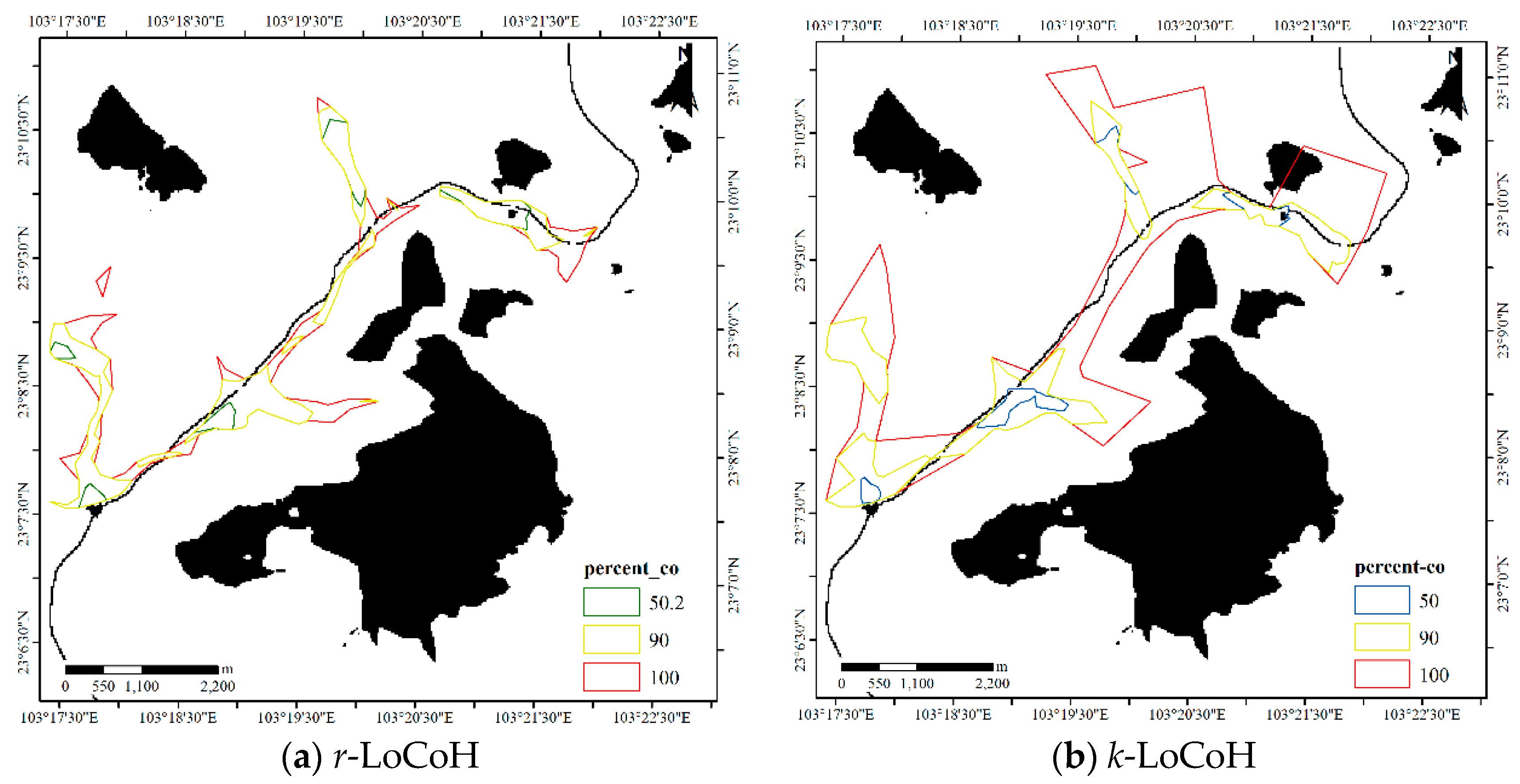
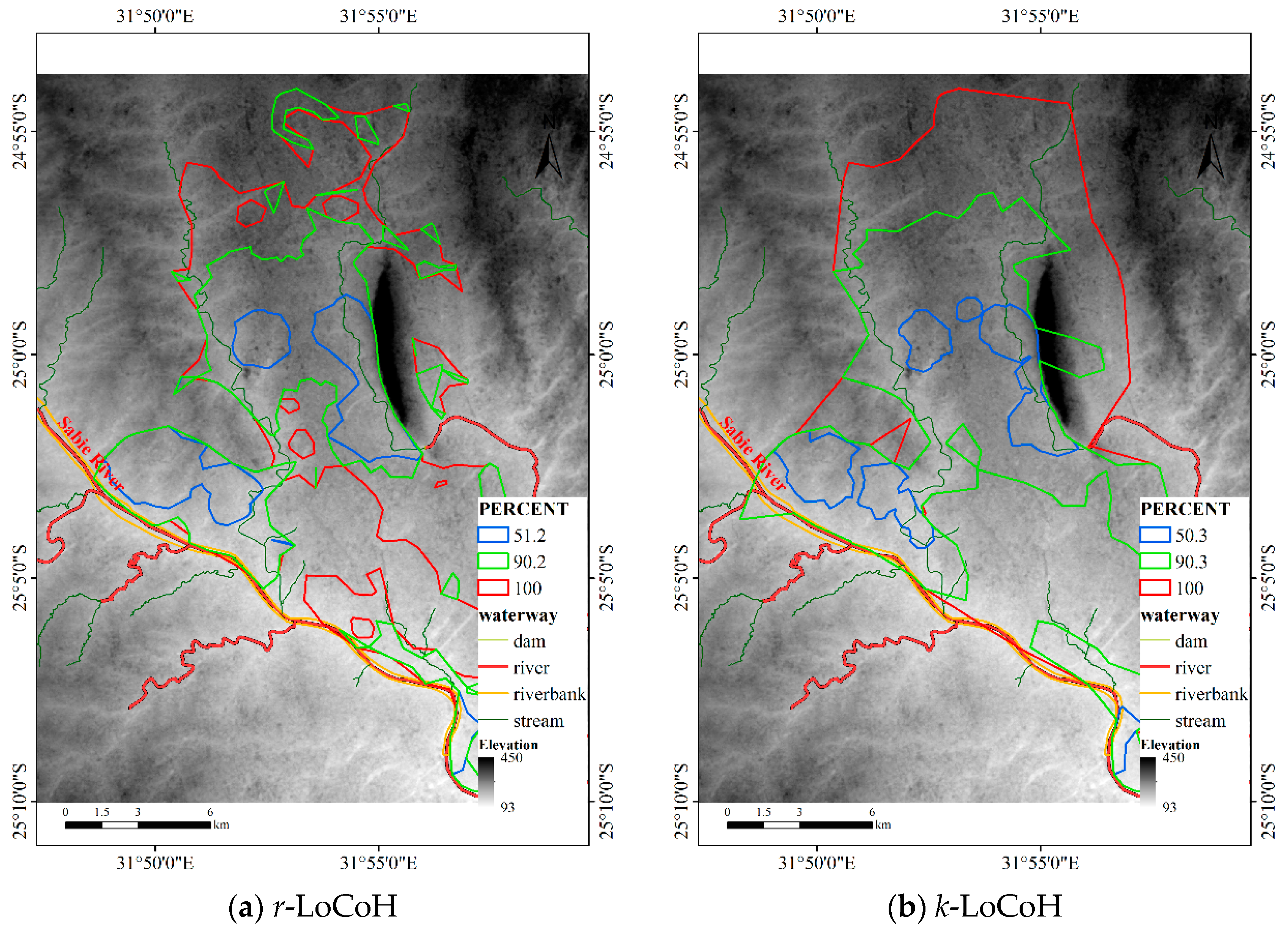
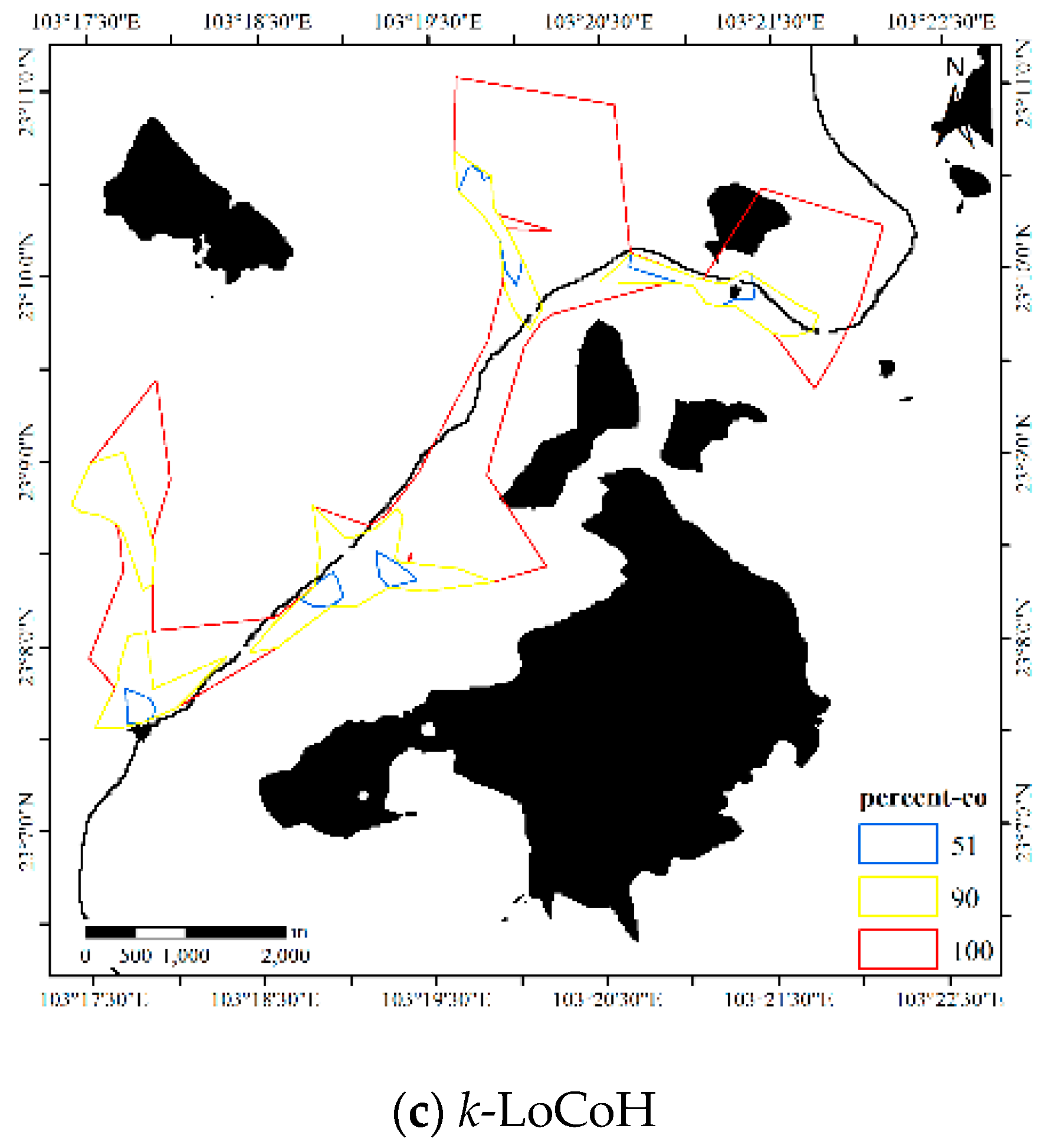
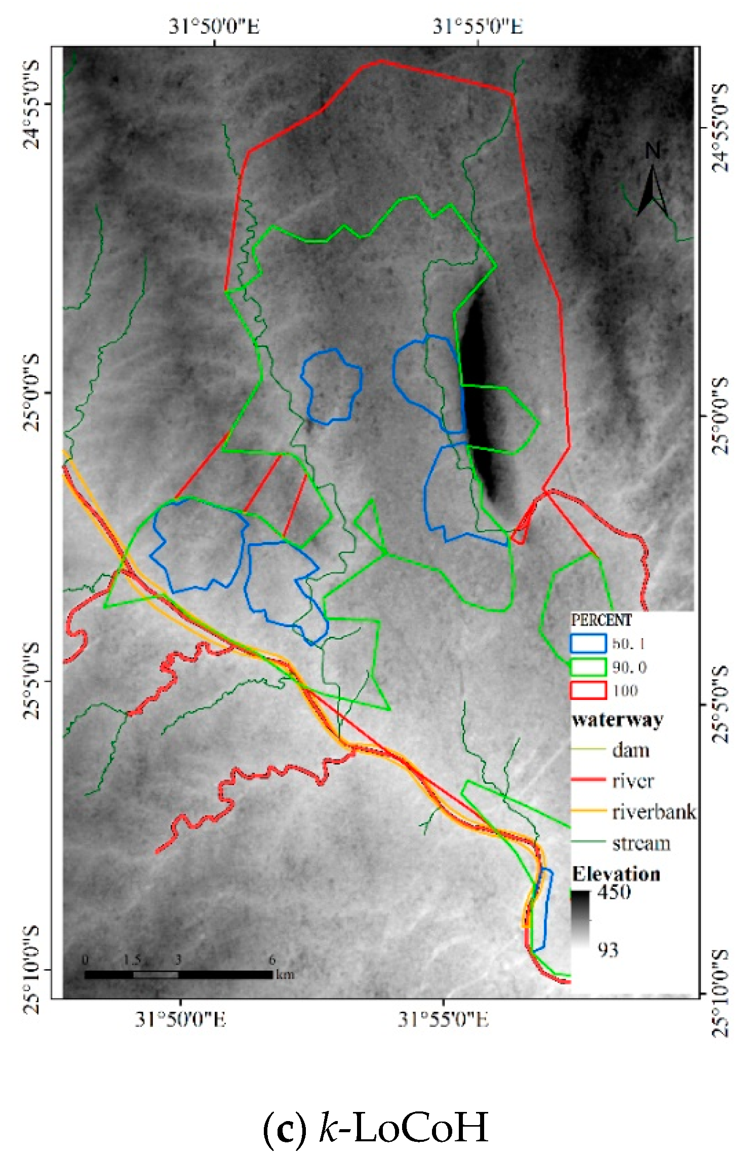
For the LoCoH method, r = 1000 m for the r-LoCoH and k = 59 for the k-LoCoH, with the results shown in Figure 18. Similar to experiment 2, the extent of the r-LoCoH result is narrower than that of other methods, but the HR of r-LoCoH is very fragmented. The result of the LoCoH method is coarser than the results of other methods, and some regions with a non-zero probability of animal activity are missing. Thus, the results of the DFHRE and KDE are better than those of LoCoH. From the perspective of the obstacles, the HR of LoCoH slightly overlaps the Sabie River, and the HR of r-LoCoH almost avoids the mountains, but the HR of k-LoCoH does not. Therefore, the results of the DFHRE and LoCoH methods are better than those of the KDE.
In summary, the proposed method can naturally represent the possibility degree or density of the distribution of an animal, bypass obstacles and consider the impact of the terrain; additionally, some areas with a non-zero possibility of animal activity can be expressed, and the two types of statistical errors are effectively reduced. According to the criteria introduced in Section 1, it can be concluded that the results of the proposed DFHRE method are better than the results of the KDE and LoCoH methods.
4.3.4. Cross Validation
In this section, the leave-one-out cross-validation method [4] is used to test the performance of the proposed method and compare it with the MKDE and k-LoCoH. The results are shown in Figure 19, Figure 20 and Figure 21, and the area changes of the results are listed in Table 4. For the DFHRE, when the number of samples is reduced to half of the original dataset, all core areas and HRs are also reduced, but no substantial changes occur. However, the result of MKDE shows the reverse trend. The results of k-LoCoH display no consistent trend, and the area of core areas based on k-LoCoH for Dataset 1 increased by 32.38%. From the perspectives of obstacles and terrain, the result of the MKDE overlaps the Sabie River and almost covers the mountain area (labeled in Figure 5). The result of LoCoH overlaps the river and the mountains. In contrast, the result of the DFHRE does not overlap the Sabie River, and the overlapping area between the HR and mountains is very small. Therefore, this cross-validation method shows that the results of the DFHRE are more stable and reasonable than those of the MKDE and k-LoCoH.
5. Conclusions
HR estimation is the basis of ecology and animal behavior research. The results of a HR estimator can illustrate the fuzzy patterns of the range of animal activity; thus, an ideal estimator should accurately describe animal activity as a fuzzy phenomenon. This paper presents a novel estimator based on the ALM. The cost distance is used to replace the Euclidean distance when the effects of terrain and obstacles need to be considered, which can effectively take into account the anisotropy of the sample points. The proposed method is implemented in Java, and three experiments and a cross-validation test show that this method can model the HRs of animals as fuzzy regions and effectively consider the terrain and avoid obstacles.
To simplify the study, we assume that animals cannot reach the obstacles and that all obstacles must be avoided. Because different land cover types may have different influences on animal activities, quantitatively determining the influence coefficients of different land cover types is important to HR estimation, especially when the land cover type is fuzzy; this topic will be explored in future work. Additionally, the spatial relationships between the HR of the oriental white stork and wetlands will also be investigated, such as topological and directional relationships. Through these spatial analyses, we can further reveal the dependence of a migratory bird on wetlands.
Author Contributions
Jifa Guo conceived of and designed the research, implemented the DFHRE algorithms in Java and wrote the manuscript. Shihong Du designed the structure of the manuscript and revised the manuscript. Zhenxing Ma completed the experiment on Datasets 1 and 3 and analyzed the results. Hongyuan Huo completed the experiment on Dataset 2, analyzed the results, and reviewed the manuscript. Guangxiong Peng compared these results with those of other methods and completed the scale analysis.
Funding
This work was supported by the Chinese National Nature Science Foundation (No. 41971410), the Key Project of the Tianjin Natural Science Foundation of China (No. 17JCZDJC39700), the Innovation Team Training Plan of the Tianjin Education Committee (No. TD13-5073) and the Hunan Natural Science Foundation of China (No. 2018JJ2502).
Acknowledgments
The authors wish to thank the anonymous reviewers who provided helpful comments on earlier drafts of the manuscript.
Conflicts of Interest
The authors declare that they have no conflict of interest to disclose.
References
- Getz, W.M.; Wilmers, C.C. A local nearest-neighbor convex-hull construction of home ranges and utilization distributions. Ecography 2004, 27, 489–505. [Google Scholar] [CrossRef] [Green Version]
- Burt, W.H. Territoriality and home range concepts as applied to mammals. J. Mammal. 1943, 24, 346–352. [Google Scholar] [CrossRef]
- Yiu, S.; Parrini, F.; Karczmarski, L.; Keith, M. Home range establishment and utilization by reintroduced lions (Panthera leo) in a small South African wildlife reserve. Integr. Zool. 2017, 12, 318–332. [Google Scholar] [CrossRef] [PubMed]
- Fleming, C.H.; Fagan, W.F.; Mueller, T.; Olson, K.A.; Leimgruber, P.; Calabrese, J.M. Rigorous home range estimation with movement data: A new autocorrelated kernel density estimator. Ecology 2015, 96, 1182–1188. [Google Scholar] [CrossRef] [PubMed]
- Schradin, C.; Schmohl, G.; Rödel, H.G.; Schoepf, I.; Treffler, S.M.; Brenner, J.; Bleeker, M.; Schubert, M.; König, B.; Pillay, N. Female home range size is regulated by resource distribution and intraspecific competition: A long-term field study. Anim. Behav. 2010, 79, 195–203. [Google Scholar] [CrossRef]
- Van Beest, F.M.; Rivrud, I.M.; Loe, L.E.; Milner, J.M.; Mysterud, A. What determines variation in home range size across spatiotemporal scales in a large browsing herbivore? J. Anim. Ecol. 2011, 80, 771–785. [Google Scholar] [CrossRef]
- Tuqa, J.H.; Funston, P.; Musyokib, C.; Ojwang, G.O.; Gichuki, N.N.; Bauer, H.; Tamis, W.; Dolrenry, S.; Van‘t Zelfde, M.; de Snoo, G.R.; et al. Impact of severe climate variability on lion home range and movement patterns in the Amboseli ecosystem, Khenya. Glob. Ecol. Conserv. 2014, 2, 1–10. [Google Scholar] [CrossRef]
- Powell, R.A. Animal Home Ranges and Territories and Home Range Estimators. In Research Techniques in Animal Ecology: Controversies and Consequences; Boitani, L., Fuller, T.K., Eds.; Columbia University Press: New York, NY, USA, 2000; pp. 65–110. [Google Scholar]
- Chirima, G.J.; Owen-Smith, N. Comparison of Kernel Density and Local Convex Hull Methods for Assessing Distribution Ranges of Large Mammalian Herbivores. Trans. GIS 2017, 21, 359–375. [Google Scholar] [CrossRef]
- Row, J.R.; Blouin-Demers, G. Kernels are not accurate estimators of home-range size for herpetofauna. Copeia 2006, 4, 797–802. [Google Scholar] [CrossRef]
- Nilsen, E.B.; Pedersen, S.; Linnell, J.D.C. Can minimum convex polygon home ranges be used to draw biologically meaningful conclusions? Ecol. Res. 2008, 23, 635–639. [Google Scholar] [CrossRef]
- Downs, J.A.; Horner, M.W. A Characteristic-Hull Based Method for Home Range Estimation. Trans. GIS 2009, 13, 527–537. [Google Scholar] [CrossRef]
- Worton, B.J. Kernel methods for estimating the utilization distribution in home-range studies. Ecology 1989, 70, 164–168. [Google Scholar] [CrossRef]
- Ostro, L.E.T.; Young, T.P.; Silver, S.C.; Koontz, F.W. A geographic information system method for estimating home range size. J. Wildl. Manag. 1999, 63, 748–755. [Google Scholar] [CrossRef]
- Getz, W.M.; Fortmann-Roe, S.; Cross, P.C.; Lyons, A.J.; Ryan, S.J.; Wilmers, C.C. LoCoH: Non-parametric kernel methods for constructing home ranges and utilization distributions. PLoS ONE 2007, 2, e207. [Google Scholar] [CrossRef]
- Horne, J.S.; Garton, E.O.; Krone, S.M.; Lewis, J.S. Analyzing animal movements using Brownian bridges. Ecology 2007, 88, 2354–2363. [Google Scholar] [CrossRef]
- Wells, A.G.; Blair, C.C.; Garton, E.O.; Rice, C.G.; Horne, J.S.; Rachlow, J.L.; Wallin, D.O. The Brownian bridge synoptic model of habitat selection and space use for animals using GPS telemetry data. Ecol. Model. 2014, 273, 242–250. [Google Scholar] [CrossRef]
- Long, J.A.; Nelson, T.A. Time Geography and Wildlife Home Range Delineation. J. Wildl. Manag. 2012, 76, 407–413. [Google Scholar] [CrossRef]
- Long, J.A. Modeling movement probabilities within heterogeneous spatial fields. J. Spat. Inf. Sci. 2018, 16, 85–116. [Google Scholar] [CrossRef]
- Kranstauber, B. Modelling animal movement as Brownian bridges with covariates. Mov. Ecol. 2019, 7, 22. [Google Scholar] [CrossRef]
- Péron, G. Modified home range kernel density estimators that take environmental interactions into account. Mov. Ecol. 2019, 7, 16. [Google Scholar] [CrossRef] [Green Version]
- Zadeh, L.A. Fuzzy sets as a basis for a theory of possibility. Fuzzy Sets Syst. 1978, 1, 3–28. [Google Scholar] [CrossRef]
- Drakopoulos, J.A. Probabilities, possibilities, and fuzzy sets. Fuzzy Sets Syst. 1995, 75, 1–15. [Google Scholar] [CrossRef]
- Dubois, D.; Prade, H.; Sandri, S. On Possibility/Probability Transformations. In Fuzzy Logic; Lowen, R., Roubens, M., Eds.; Springer: Dordrecht, The Netherlands, 1993; pp. 103–112. [Google Scholar]
- Shouraki, S.B.; Honda, N. Recursive fuzzy modeling based on fuzzy interpolation. J. Adv. Comput. Intell. 1999, 3, 114–125. [Google Scholar] [CrossRef]
- Li, J.; Li, Y.; Miao, L.; Xie, G.; Yuan, F. A Comparison of Autumn Habitat Selection of Cervus nippon and Sus scrofa in Taohongling National Nature Reserve, China. Sichuan J. Zool. 2015, 34, 300–305. [Google Scholar]
- Zhang, S.; Guo, R.; Liu, W.; Weng, D.; Cheng, Z. Research Progress and Prospect of Cervus nippon kopschi. J. Zhejiang For. Sci. Technol. 2016, 36, 90–94. [Google Scholar]
- Calabrese, J.M.; Fleming, C.H.; Gurarie, E. ctmm: An R package for analyzing animal relocation data as a continuous-time stochastic process. Methods Ecol. Evol. 2016, 7, 1124–1132. [Google Scholar] [CrossRef]
- Yang, C.; Hu, H.; Hu, P.; Cao, F. Solution of Euclidean Shortest Path Problem Space with Obstacles. Geomat. Inf. Sci. Wuhan Univers. 2012, 37, 1495–1499. [Google Scholar]
- Lele, S.R.; Keim, L.L. Weighted distributions and estimation of resource selection probability functions. Ecology 2006, 87, 3021–3028. [Google Scholar] [CrossRef]
- Horne, J.S.; Garton, E.O.; Rachlow, J.L. A synoptic model of animal space use: Simultaneous estimation of home range, habitat selection, and inter/intra-specific relationships. Ecol. Model. 2008, 214, 338–348. [Google Scholar] [CrossRef]
- Merrikh-Bayat, F.; Shouraki, S.B. The neuro-fuzzy computing system with the capacity of implementation on a memristor crossbar and optimization-free hardware training. IEEE Trans. Fuzzy Syst. 2014, 22, 1272–1287. [Google Scholar] [CrossRef]
- Javadian, M.; Shouraki, S.; Kourabbaslou, S.S. A novel density-based fuzzy clustering algorithm for low dimensional feature space. Fuzzy Sets Syst. 2017, 318, 34–55. [Google Scholar] [CrossRef]
- Adriaensen, F.; Chardon, J.P.; De Blust, G.; Swinnen, E.; Villalba, S.; Gulinck, H.; Matthysn, E. The application of ‘least-cost’ modelling as a functional landscape model. Landsc. Urban Plan. 2003, 64, 233–247. [Google Scholar] [CrossRef]
- Becker, D.; de Andrés-Herrero, M.; Willmes, C.; Weniger, G.; Bareth, G. Investigating the Influence of Different DEMs on GIS-Based Cost Distance Modeling for Site Catchment Analysis of Prehistoric Sites in Andalusia. ISPRS Int. J. Geo-Inf. 2017, 6, 36. [Google Scholar] [CrossRef]
- Downs, J.A.; Heller, J.H.; Loraamm, R.; Stein, D.O.; McDaniel, C.; Onorato, D. Accuracy of home range estimators for homogeneous and inhomogeneous point patterns. Ecol. Model. 2012, 225, 66–73. [Google Scholar] [CrossRef]
- Downs, J.A.; Horner, M.W.; Tucker, A.D. Time-geographic density estimation for home range analysis. Ann. GIS 2011, 17, 163–171. [Google Scholar] [CrossRef]
- Steiniger, S.; Hunter, A.J.S. OpenJUMP HoRAE—A free GIS and Toolbox for Home-Range Analysis. Wildl. Soc. Bull. 2012, 36, 600–608. [Google Scholar] [CrossRef]
- Berger, K.M.; Gese, E.M. Does interference competition with wolves limit the distribution and abundance of coyotes? J. Anim. Ecol. 2007, 76, 1075–1085. [Google Scholar] [CrossRef] [Green Version]
- Chacón, J.E.; Duong, T. Multivariate plug-in bandwidth selection with unconstrained pilot bandwidth matrices. Test 2010, 19, 375–398. [Google Scholar] [CrossRef]
- Chacón, J.E.; Duong, T. Multivariate Kernel Smoothing and Its Applications; Chapman & Hall: Boca Raton, FL, USA, 2018. [Google Scholar]
- Rodgers, A.R.; Kie, J.G.; Wright, D.; Beyer, H.L.; Carr, A.P. HRT: Home Range Tools for ArcGIS. Version 2.0; Ontario Ministry of Natural Resources and Forestry, Centre for Northern Forest Ecosystem Research: Thunder Bay, ON, Canada, 2015.
- Geotools. Available online: https://geotools.org/ (accessed on 19 February 2018).
Figure 1.
The potential location and path of an animal.

Figure 2.
The rescued oriental white stork (a) and monitoring points in the spring (b).

Figure 3.
Simulated sika deer dataset.

Figure 4.
Obstacles to sika deer activities.

Figure 5.
The position locations for Cilla.

Figure 6.
The density-based fuzzy home range estimator (DFHRE) flowchart.

Figure 7.
Cost distance to original point 1 in raster space.

Figure 8.
Scan process in the map algebra-distance transformation with obstacles (MA-DTO) algorithm. (a) Eight neighbors of target cell ; (b) the scanning order from top to bottom; and (c) the scanning order from bottom to top.
Figure 8.
Scan process in the map algebra-distance transformation with obstacles (MA-DTO) algorithm. (a) Eight neighbors of target cell ; (b) the scanning order from top to bottom; and (c) the scanning order from bottom to top.

Figure 9.
The influence area of source point 1 induced by the Euclidean distance and the cost distance, respectively.
Figure 9.
The influence area of source point 1 induced by the Euclidean distance and the cost distance, respectively.

Figure 10.
The membership grade, core areas and home ranges (HRs) of Dataset 1.

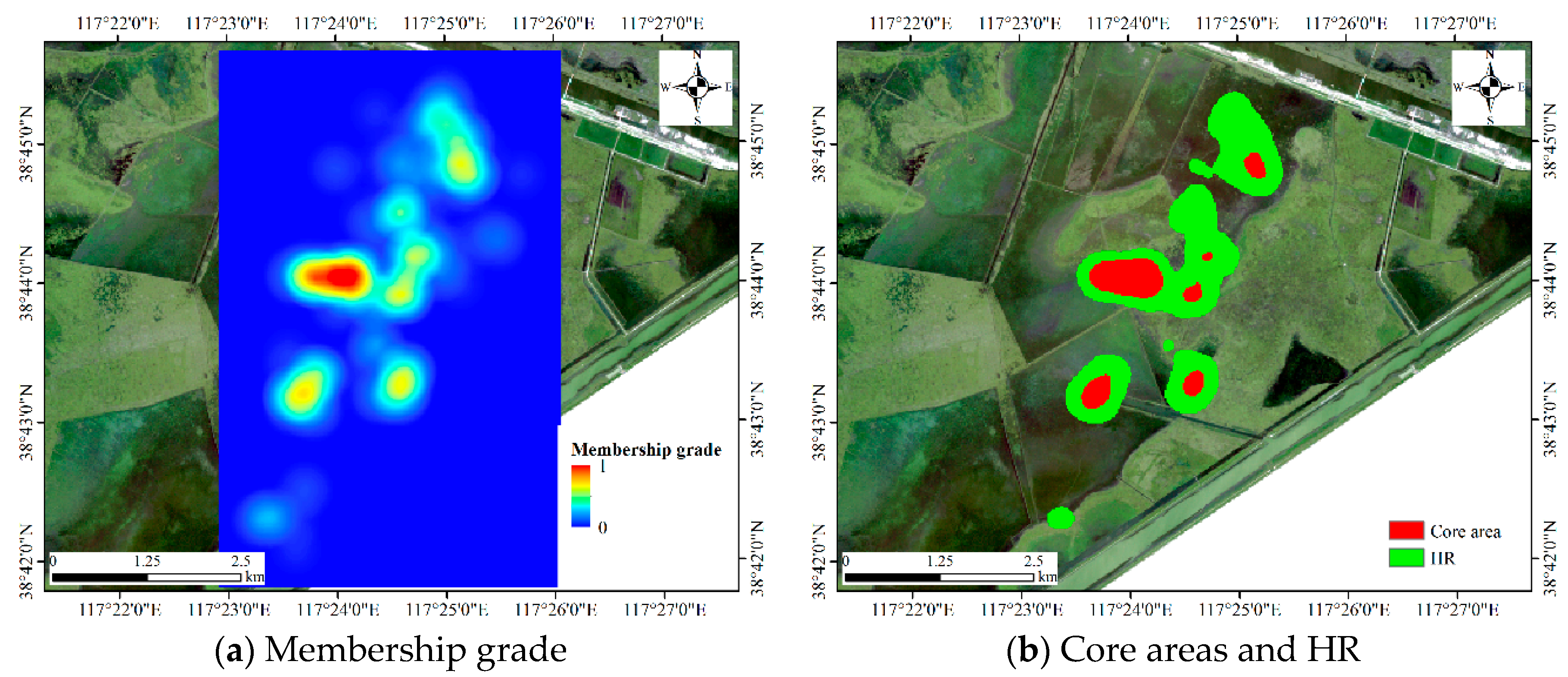
Figure 11.
The membership grade, core areas and HR of Dataset 2.

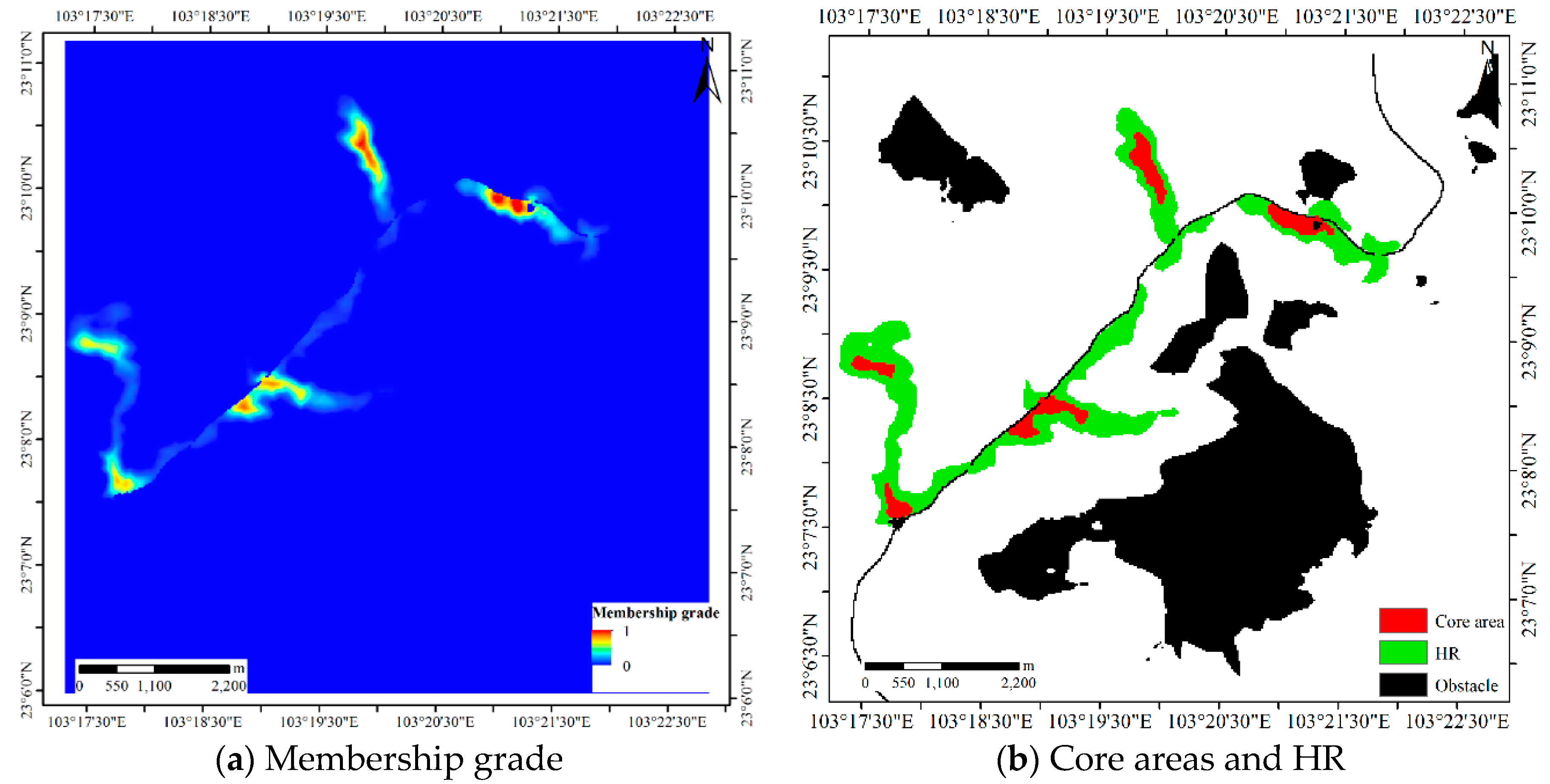
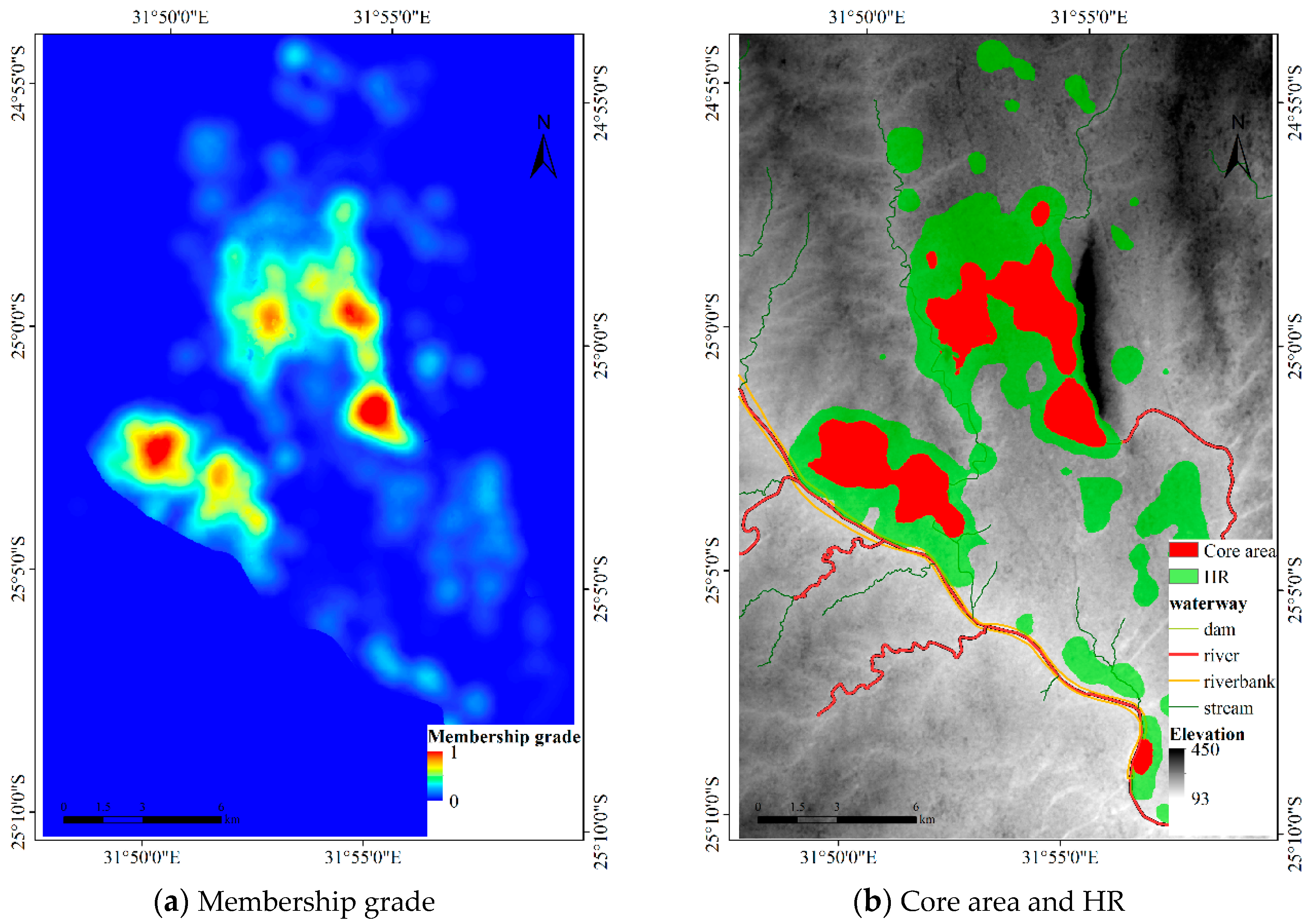
Figure 12.
The membership grade, core areas and HR of Dataset 3.

Figure 13.
HRs estimated by the kernel density-based estimator (KDE) methods for Dataset 1.

Figure 14.
HRs estimated by the LoCoH methods for Dataset 1.

Figure 15.
HR of the KDE methods for Dataset 2.

Figure 16.
HRs from the LoCoH methods for Dataset 2.

Figure 17.
HR of the KDE methods for Dataset 3.

Figure 18.
HRs of the LoCoH method for Dataset 3.

Figure 19.
HRs of the DFHRE, multivariate kernel density estimation (MKDE) and k-LoCoH methods for Dataset 1.
Figure 19.
HRs of the DFHRE, multivariate kernel density estimation (MKDE) and k-LoCoH methods for Dataset 1.

Figure 20.
HRs of the DFHRE, MKDE and k-LoCoH methods for Dataset 2.


Figure 21.
HRs of the DFHRE, MKDE and k-LoCoH methods for Dataset 3.


Table 1.
Sizes of the core areas and HRs estimated by the DFHRE, KDE and LoCoH methods for Dataset 1.
Table 1.
Sizes of the core areas and HRs estimated by the DFHRE, KDE and LoCoH methods for Dataset 1.
| Method | Core Area (m2) | HR (m2) |
|---|---|---|
| DFHRE | 754,400 | 4,124,000 |
| Fixed kernel | 738,432 | 42,23,832 |
| Adaptive kernel | 4,340,866 | 12,513,091 |
| r-LoCoH (r = 500) | 723,752 | 2,118,506 |
| k-LoCoH (k = 16) | 247,620 | 1,736,049 |
Table 2.
Sizes of the core areas and HRs estimated by the DFHRE, KDE and LoCoH methods for Dataset 2.
Table 2.
Sizes of the core areas and HRs estimated by the DFHRE, KDE and LoCoH methods for Dataset 2.
| Isopleth | Core Area (m2) | HR (m2) |
|---|---|---|
| DFHRE | 813,750 | 366,8125 |
| Fixed kernel | 1,251,385 | 7,339,245 |
| Adaptive kernel | 1,544,052 | 6,826,268 |
| r-LoCoH (r = 500) | 868,200 | 2,655,871 |
| k-LoCoH (k = 16) | 682,955 | 3,524,019 |
Table 3.
Sizes of the core areas and HRs estimated by the DFHRE, KDE and LoCoH methods for Dataset 3.
Table 3.
Sizes of the core areas and HRs estimated by the DFHRE, KDE and LoCoH methods for Dataset 3.
| Isopleth | Core Area (m2) | HR (m2) |
|---|---|---|
| DFHRE | 29,290,500 | 101,241,000 |
| Fixed kernel | 31,807,074 | 124,029,946 |
| Adaptive kernel | 60,533,862 | 232,011,617 |
| r-LoCoH (r = 1000) | 32,101,265 | 90,196,218 |
| k-LoCoH (k = 59) | 26,282,337 | 126,126,900 |
Table 4.
Area changes in the results of the DFHRE, MKDE, and k-LoCoH for the three datasets.
| Data | Method | Core | HR | ||||
|---|---|---|---|---|---|---|---|
| Full (m2) | Half (m2) | Reduction (%) | Full (m2) | Half (m2) | Reduction (%) | ||
| Dataset 1 | DFHRE | 754,400 | 711,200 | 5.73% | 4,124,000 | 3,479,600 | 15.63% |
| MKDE | 738,432 | 940,039 | −27.30% | 4,223,832 | 5,313,703 | −25.80% | |
| k-LoCoH | 247,620 | 327,806 | −32.38% | 1,736,049 | 1,890,265 | −8.88% | |
| Dataset 2 | DFHRE | 813,750 | 808,750 | 0.61% | 3,668,125 | 3,211,250 | 12.46% |
| MKDE | 1251,385 | 1,529,783 | −22.25% | 7,339,245 | 8,027,278 | −9.37% | |
| k-LoCoH | 682,955 | 639,636 | 6.34% | 3,524,019 | 2,834,798 | 19.56% | |
| Dataset 3 | DFHRE | 29,290,500 | 27,856,800 | 4.89% | 101,241,000 | 95,163,300 | 6.00% |
| MKDE | 31,807,074 | 33,326,862 | −4.78% | 124,029,946 | 134,312,919 | −8.29% | |
| k-LoCoH | 26,282,337 | 26,145,740 | 0.52% | 126,126,900 | 124,467,800 | 1.32% | |
© 2019 by the authors. Licensee MDPI, Basel, Switzerland. This article is an open access article distributed under the terms and conditions of the Creative Commons Attribution (CC BY) license (http://creativecommons.org/licenses/by/4.0/).
Share and Cite
MDPI and ACS Style
Guo, J.; Du, S.; Ma, Z.; Huo, H.; Peng, G. A Model for Animal Home Range Estimation Based on the Active Learning Method. ISPRS Int. J. Geo-Inf. 2019, 8, 490. https://0-doi-org.brum.beds.ac.uk/10.3390/ijgi8110490
AMA Style
Guo J, Du S, Ma Z, Huo H, Peng G. A Model for Animal Home Range Estimation Based on the Active Learning Method. ISPRS International Journal of Geo-Information. 2019; 8(11):490. https://0-doi-org.brum.beds.ac.uk/10.3390/ijgi8110490
Chicago/Turabian StyleGuo, Jifa, Shihong Du, Zhenxing Ma, Hongyuan Huo, and Guangxiong Peng. 2019. "A Model for Animal Home Range Estimation Based on the Active Learning Method" ISPRS International Journal of Geo-Information 8, no. 11: 490. https://0-doi-org.brum.beds.ac.uk/10.3390/ijgi8110490
Note that from the first issue of 2016, this journal uses article numbers instead of page numbers. See further details here.