Article

Study of NSSDA Variability by Means of Automatic Positional Accuracy Assessment Methods

by
Juan José Ruiz-Lendínez
*,
Francisco Javier Ariza-López
and
Manuel Antonio Ureña-Cámara
Department of Cartographic Engineering, University of Jaén, 23071 Jaén, Spain
*
Author to whom correspondence should be addressed.
ISPRS Int. J. Geo-Inf. 2019, 8(12), 552; https://0-doi-org.brum.beds.ac.uk/10.3390/ijgi8120552
Submission received: 18 September 2019 / Revised: 27 November 2019 / Accepted: 2 December 2019 / Published: 2 December 2019

Abstract

:
Point-based standard methodologies (PBSM) suggest using ‘at least 20’ check points in order to assess the positional accuracy of a certain spatial dataset. However, the reason for decreasing the number of checkpoints to 20 is not elaborated upon in the original documents provided by the mapping agencies which develop these methodologies. By means of theoretical analysis and experimental tests, several authors and studies have demonstrated that this limited number of points is clearly insufficient. Using the point-based methodology for the automatic positional accuracy assessment of spatial data developed in our previous study Ruiz-Lendínez, et al (2017) and specifically, a subset of check points obtained from the application of this methodology to two urban spatial datasets, the variability of National Standard for Spatial Data Accuracy (NSSDA) estimations has been analyzed according to sample size. The results show that the variability of NSSDA estimations decreases when the number of check points increases, and also that these estimations have a tendency to underestimate accuracy. Finally, the graphical representation of the results can be employed in order to give some guidance on the recommended sample size when PBSMs are used.

1. Introduction

The position is the basis of mapping and navigation, which are essential for engineering, natural sciences, land management, etc. Consequently, the assessment of the positional quality of cartographic products has become an issue of particular significance and relevance [1,2]. Positional quality is determined by positional accuracy [3] which, in turn, is evaluated by means of statistical methods based on measuring positional discrepancies between the location of “well-defined point entities” stored in a geospatial database (GDB) and their true (real world) location [1]. In this sense, there are several point-based standard methodologies (PBSM) which can be used for computing the positional accuracy of GDBs. In these methodologies the positional accuracy is estimated by means of a statistical evaluation of random and systematic errors and mainly specified through two metrics or estimators: root mean square error (RMSE) (Figure 1) or mean value of errors (μ), and their standard deviation (σ) [4,5]. Among the PBSM which can be employed for defining the positional accuracy of spatial data we highlight: The National Map Accuracy Standard (NMAS) developed in 1947 by the US Bureau of the Budget [6], the Engineering Map Accuracy Standard (EMAS) developed in 1983 by the Committee on Cartographic Surveying of the American Society of Civil Engineering [7], and the National Standard for Spatial Data Accuracy (NSSDA) published in 1998 by the Federal Geographic Data Committee [8].
All these PBSM are different from each other and give results in varied ways. Thus, while EMAS and NMAS propose the direct approval/rejection of the cartographic product, the NSSDA gives results in an open way, leaving up to the user´s criteria whether or not the derived accuracy reaches his/her expectations [4]. However, and despite these differences, all of these PBSM share a common aspect which is controversial: their recommendations on the size of the sample. In this sense, all of them suggest using ‘at least 20’ check points in order to assess the positional accuracy of a certain GDB. However, the reason for decreasing the number of check points to 20 is not clear, also taking into account that the size of the area to assess is not specified with sufficient detail (In this regard, several options such as spatial framework, project, product, sheet, or map are used to refer to their geographical scope of application). In any case, and from a statistical point of view, this limited number of points is clearly insufficient. This is evidenced by several authors and institutions [4,5,10,11,12,13,14]. Specifically, and taking as a point of reference the work of Ley [10] related to the accuracy assessment of digital terrain models (DTM), Li [5] discusses the effects of the characteristics—accuracy, number, and distribution—of the set of check points used for experimental tests of DTM accuracy on the resulting accuracy figures. These effects are investigated both through a theoretical analysis and by experimental tests, concluding that “only if the sample size is increased and the accuracy of the check points is improved at the same time, can the reliability of the final estimates be improved”. Following the line of argument adopted by Li; Ariza and Atkinson [4] analyze the variability of NSSDA estimations using a statistical simulation process. These authors replicate the NSSDA application process under controlled circumstances by means of synthetic normal distributed populations of errors. This simulation process shows both that the NSSDA has a small tendency to underestimate accuracy, and that the use of samples of at least 100 points is needed in order to reach an effective confidence level of 95%. According to Ariza and Atkinson´s conclusions, Zandbergen [14] also recommends the use of sample sizes greater than 20 locations when applying NSSDA because this size seems insufficient considering the variability and complexity of many positional error distributions.
Overall, it seems obvious that the inclusion of more check points in the positional accuracy assessment procedures will lead to a more reliable result. Therefore, it can be said that an adequate sample size is determined by the degree of confidence or the reliability requirement on the final accuracy estimates [5]. In other words, the number of points should be large enough to ensure, with a given level of confidence, that a GDB with an unacceptable quality level will not be acquired [4].
In contrast to the above evidence, it is also true that a large number of check points involve a very high cost of field surveying [15], despite efficiency improvement of the field data acquisition processes provided by global navigation satellite systems (GNSS). This circumstance has favored the development of new approaches aimed at increasing the automation level of the positional accuracy assessment procedures. These approaches are based on the method of defining positional accuracy proposed by Goodchild and Hunter [16], who suggest quantifying the positional accuracy of a certain GDB by measuring the differences between the locations of spatial entities stored in that GDB (named as tested or assessed data sources) and their locations determined by another GDB (named as reference data sources) of greater accuracy. Based on this ‘new’ paradigm, we have developed a point-based methodology for the automatic positional accuracy assessment (APAA) of spatial data [1,9]. This methodology has allowed us not only to increase significantly the number of entities (points) used in the assessment process (by means of the PBSM application) but also to empirically verify the conclusions reached by Ariza and Atkinson [4] with regard to the variability of NSSDA estimations, without the need to generate synthetic populations of errors, when the number of check points increases.
This paper takes as its starting point our previous work [1]. Specifically, a subset of the homologous points obtained between two urban GDBs according to the automated methodology developed in it, and is focused on the second aspect mentioned above, that is, to verify that the variability of NSSDA results decreases when the number of check points increases, and their tendency to underestimate accuracy. To this end, and starting from the aforementioned set of homologous points (check points population), we have applied the NSSDA standard for assessing the positional accuracy to different sample sizes. Just as a reminder, it must be noted that the calculation of these homologous points was developed in two main steps (Figure 2): (i) Matching of polygonal shapes (buildings) between the two datasets by means of an inter-elements similarity quantification procedure (Figure 2a). This procedure is based on a weight-based classification methodology using low-level polygon feature descriptors and a genetic algorithm [17], and (ii) the matching of points by means of an intra-elements metric for comparing two polygonal shapes (Figure 2b). This metric is based on a procedure developed by Arkin et al. [18] which compares two polygonal curves by means of their turn angle representations.
As already stated, both procedures are extensively detailed in [1]. It is, therefore, necessary to emphasize that they are not addressed here. In this study we focus on reproducing the experiment of Ariza and Atkinson [4] employing a population of errors automatically obtained from true—or real—locations. Therein lies the main innovative features of our methodological approach: (i) in the use of a check points population that is automatically generated, which ensures that there is no selection bias; (ii) in the use and manipulation of large volumes of empirical data (what is currently known as big data analysis) in order to verify the validity of the experiments developed by means of traditional tools from synthetic data—as in the case of [4]; (iii) in the specific characteristics of APAA procedures because the collection, management, processing, and analysis of the empirical data is cheap, quick, and requires a low computational time compared to traditional methodologies (especially if we consider fieldwork for GNSS data acquisition). On the other hand, our results should serve to convincingly demonstrate that the proposals and suggestions made by some of the authors and institutions above mentioned [4,12,13,14] have contributed significantly to improve the technical definition of the NSSDA in aspects which require special attention, such as:
  • Give information about the statistical behavior of the methodology.
  • Related to the previous, give a clear and better recommendation about the number and distribution of check points and their influence on the variability and reliability of results.
Finally, our study pays special attention to the characterization of the distribution of positional error. As will be explained below, a key assumption of the NSSDA standard is that the positional errors follow a normal distribution; which is also assumed by the experiment of Ariza and Atkinson [4]. However, the non-normal distribution of positional error observed in several applications presents a serious challenge to map accuracy standards, which rely on assumptions of normality and utilize simple statistics to characterize its distribution.
The rest of the paper is organized in the following main sections: the next section presents the urban databases used and the conditions that needed to be fulfilled by them in order to apply our methodology as well as the homologous points population (check points). After this, the following section explains the sampling procedure with a particular focus on normality testing on the population distribution, and the sample design and composition. Following this, effects of the sample size and sample distribution on the automatic positional accuracy estimations by means NSSDA are presented and discussed in the next section. Finally, general conclusions are presented.

2. Urban Databases Used and Points Population

As already mentioned, our APAA procedure [9] quantifies positional accuracy by measuring the positional discrepancies (Hereinafter referred to as errors (statistical estimators we are going to work with)) between the locations of “well-defined punctual entities” stored in two GDBs —tested and reference. However, there are some conditions that need to be fulfilled by any two spatial datasets in order to apply our approach. A large part of these conditions or constraints is closely linked to the interoperability between these datasets.
From a cartographic point of view, interoperability can be defined as the capability that two spatial datasets—from different sources—have to interact with each other [19]. According to this, the positional component seems essential to achieving a satisfactory level of interoperability. So much so that some authors, such as Giordano and Veregin [20], prefer to use the term Confrontability, defining it as the level at which it is possible to operate with spatial datasets that occupy the same geographical region, that is to say, the same spatial position. However, there are some other aspects that must be considered—apart from position—in order to assure interoperability between spatial data. Thus, in our specific case interoperability must also be guaranteed to two other levels: semantic and topological. Therefore, for the implementation of our APAA procedure, two GDBs must not only occupy the same geographic region and be mapped with the same coordinate reference system (CRS), but there must also be semantic homogeneity (i.e., no differences in the intended meaning of terms in specific contexts [1]), and their topological relationships must be preserved. Apart from this, the two GDBs must meet two obvious constraints: (i) all the elements used must exist in both datasets (the coexistence constraint), and (ii) both datasets must be independently produced (the independence constraint). The first constraint, despite its logic, is not always fulfilled in the real world, since two GDBs generated at different scales are normally not at the same level of generalization. With regard to the second one, neither of the two GDBs can be derived from another cartographic product of a larger scale through any process, such as generalization, which means that their quality has not been degraded.
With regard to specific cartographic products, we have used two official cartographic databases in Andalusia (Southern Spain). As the tested source we have used the BCN25 (“Base Cartográfica Numérica E25k”) and as the reference source, we have used the MTA10 (“Mapa Topográfico de Andalucía E10k”). Both GDBs are presented as a set of vector covers distributed by layers, including a vector layer of buildings (city-blocks) that contains the same type of geometrical information. Their description, the degree of fulfillment of the previously mentioned interoperability requirements, as well as the justification for the selection of features—buildings as polygonal features for developing the inter-elements matching procedure and the vertexes which define their contour as well-defined punctual features for assessing the positional accuracy—are provided in detail in [1,2], so once again we must note that these issues will not be addressed here. With regard to the independence and coexistence constraints, both GDBs were independently produced which means that the tested source (BCN25) is not derived from the reference source (MTA10), and thanks to the limitations imposed by the matching methodology used—through a matching accuracy indicator [1]—all the elements used in our APAA procedure exist in both datasets. This last indicator also avoids—with a confidence level of 95% [1]—matching between non-homologous pairs of points. This assertion was also corroborated by means of a visual inspection procedure.
Finally, and with regard to the urban area selected, this is included in sheet number 1009-IV of the MTN25k—National Topographic Map of Spain at scale 1:25000—belonging to the city of Granada (Andalusia, Spain) and covered by both the BCN25 and the MTA10. This area is coded as 1009_07 and 1009_08 in our previous study [1] (Figure 3). The reason for choosing these databases is twofold: (i) Because of their size, since they provide a great number of matched features, both polygons (buildings), and points (vertexes which define their boundary). This characteristic is essential to extracting samples with a range of sizes that allows us to analyze the variability of NSSDA results according to the conditions established in [4]; and (ii) because of their strictly urban nature, since they offer a wide range of building types which means a huge variety with respect to the shape and size of the polygons that integrate them. This increases the probability of pairing polygons that provide a high number of check points. This last characteristic is very useful for analyzing the effect of sample distribution on the NSSDA results.
Table 1 shows the total number of polygons comprising these databases, the number of polygons matched, as well as the homologous points population (denoted as matched vertexes) computed for them (input data for this study). According to the data presented in this table, and despite being a very large number, the homologous points population represented by the number of matched vertexes constitutes a relatively low percentage compared to the total number of vertexes, reaching values of around 30% for BCN25 and 15% in the case of MTA10. As stated above, this is due both to the limitations imposed by the matching methodology used and to certain factors such as the level of detail associated with the scale at which each product is generated. Such is the case of the polygons highlighted in Figure 4c. These three polygons which are composed of four vertexes each on the BCN25 are represented by means of much more complex shapes on the MTA10. Thus, although the three polygons are matched according to our inter-elements matching procedure—they are filled in black in Figure 4a,b—they do not add any homologous point after applying the intra-elements metric. In any case, this also avoids including erroneous check points in our APAA procedure.

3. Sampling Procedure

3.1. Normality Testing

Normality is the most widely-assumed hypothesis in the case of control of quantitative variables and, in the specific case of mapping, positional error is not an exception [5,21,22,23]. Thus, one key assumption of the NSSDA standard is that the data do not contain any systematic errors and that the positional errors follow a normal distribution. However, this assumption has not undergone much testing and is not elaborated upon in the original Federal Geographic Data Committee (FGDC) documents on NSSDA [14]. Even some authors [24] have criticized as inappropriate the Greenwalt and Schutz [25] approximations used in the NSSDA, in particular when the values for RMSE(x) and RMSE(y) are very different, or when the error distribution in the x and y directions are not independent. Furthermore, there is strong evidence to suggest that many spatial data types are not normally distributed. In this sense, Zandbergen [14] performs—as a preliminary step for the development of his own analysis—an interesting review of several empirical studies that examine the distribution of positional error in different types of spatial data. According to this review, while the studies of Vonderohe and Chrisman [26] on the positional error of USGS digital line graphs data, and Bolstad et al. [27] on the accuracy of manually digitized map data show evidence of non-normality or find statistically significant differences between the observed error distribution and a normal distribution, several other studies mainly developed by members of the Institut Géographique National (IGN)—the French Mapping Agency—including studies by Vauglin [28] and Bel Hadj Ali [29] on the positional accuracy of lines and areas, suggest that the error distribution is largely normal.
In the view of such variable results, in his own study Zandbergen [14] focuses his attention on the development of a rigorous characterization of the positional error distribution in four different types of spatial data: GPS locations, street geocoding, TIGER roads, and LIDAR elevation data; concluding that in all cases the positional error could be approximated with a normal distribution, although there is some evidence of non-stationary behaviors resulting in a lack of normality. More recent studies [30,31,32,33,34] follow the line of argument adopted by Zandbergen in his work defending that positional errors could be not normally distributed. Among these last studies, Ariza-López et al. [34] argue that there are six main causes of the non-normality of many positional error distributions: (i) the presence of too many extreme values (i.e., outliers), (ii) the overlap of two or more processes, (iii) insufficient data discrimination (e.g., round-off errors, poor resolution), (iv) the elimination of data from the sample, (v) the distribution of values close to zero or the natural limit, and (vi) data following a different distribution. The presence of any of these cases can have several consequences depending on the degree of non-normality of the data and the robustness of the method applied. In the specific case of the positional errors obtained by means of our APAA procedure the incidence of the causes aforementioned is minimized thanks mainly to the limitations imposed by the matching procedures employed—through a matching accuracy indicator [1]. We must note that this is another important advantage of our approach compared to traditional methodologies. In any case, the simulation process developed by Ariza and Atkinson [4] was performed using a normal N ( μ P = 0 ;   σ P 2 = 1 ) distributed population of errors, so in order to reproduce their experiment under similar conditions it was necessary to carry out data analysis to verify their normal distribution.
Compared to other studies where the small sample sizes do not allow for proper distribution testing [35], for our research we had available a population large enough (4046 pairs of homologous points) to assess whether it followed a normal distribution. For this purpose, we used the Kolmogorov–Smirnov test [36]. This test examines whether a variable follows a given distribution in a population. This “given distribution” is usually, but not always, the normal distribution. With regard to the results, they show that the similitude is statistically significant, specifically, the obtained values are frequency distance: 0.120; Z-Kolmogorov: 0.595, and p-value: 0.875. Moreover, they have been reported from a graphic point of view by means of the histograms of the x and y components. Figure 5 shows the x and y components of errors separately, and visually it appears both distributions are very close to normal. In addition, the distributions are very symmetrical. In any case, this result should be interpreted with caution considering the variability and complexity of error distributions of these spatial data types.

3.2. Sample Design

One of the most controversial aspects of all the PBSM is the spatial distribution of control elements because, among other things, it could condition the validity of the sampling procedure [4]. In this regard, we must note that the related literature is scarce, so there are few references and, in any case, they refer to other types of cartographic products. As an example, in the specific case of the accuracy assessment of DTMs, the main research efforts have been focused on determining the best option with regard to the distribution of check points [5,37,38,39]. Thus, while some authors, and institutions such as the ISPRS, prefer to distribute the check points in a grid pattern, others consider that the sample of heights should be randomly selected from the entire model. Furthermore, some additional conditions are also established such as that the control points must be located at a certain distance from structural elements of the terrain and taken in flat areas or areas of uniform slope, less than 20% [40].
With regard to the case of planimetric data, most of the PBSMs indicate very briefly what the most appropriate distribution of check points must be, and only in a few cases a proposal of distribution agreed between producer and user is recommended [41]. Thus, the main suggested guidelines are based on the specific recommendations provided by the FGDC [8]. These recommendations are subjected to compliance with some requirements, such as the homogeneity of the area to assess with regard to the importance of their components and the homogeneous behavior of the uncertainty [42]. According to these recommendations, the points have to be located with a minimum distance between each point and the next of at least 10% of the greater diagonal of the study area. Moreover, each quadrant of the study area has to contain more than 20% of the total number of check points (Figure 6a) [8].
In our case, in order to have an adequate representation of the assessment a sample design with a robust statistical basis was necessary. This design should produce an unbiased estimate, being robust to different population spatial patterns and densities. To this end, and according to the PBSM’s recommendations, a grid sampling pattern was defined (covering all the terrain) where samples (pairs of homologous points) were randomly collected within each cell generated (Figure 6b). With regard to the grid configuration, the number of cells and their size will depend on the geographical area covered and the size of the sample. In our case, this number was set for each sampling procedure. Thus, if a sample is composed of 25 points the geographical area covered by the study GDB will be divided into a grid of 5 × 5 cells, so that as far as possible, a homogeneous distribution of the points according to the cited specifications is produced. In addition, in order to avoid biasing the final results obtained when the effect of sample size on NSSDA estimations is analyzed, and wherever possible, only one point by polygon was used. Such is the case for a polygon that occupies part of two or more cells of the sampling grid (Figure 6b). Thus, if we select the vertex V1 belonging to the highlighted polygon and included in the cell D4 to calculate the positional accuracy, we may not use the vertex V2 (included in the cell E4) because it belongs to the same polygon. In this case, we must use another vertex, V3, to be included in any other polygon.

3.3. Sample Sizes and Application of the NSSDA Standard

With regard to the sizes of the sample (n) and in order, once again, to reproduce the experiment of Ariza and Atkinson [4] under similar conditions, we used 18 different sizes between n = 10 and n = 500 and with the following distribution: from n = 10 to n = 100 the Δn was set to 10, and from n = 150 to n = 500 the Δn was set to 50. In addition, for each sample size (n = 10, 20, 30, etc.) the number of random samples used was 1000. Finally, for each sample size resulting values of NSSDA accuracies were aggregated, deriving means and deviations variability. Table 2 summarizes the steps for applying the NSSDA standard.
It must be noted that this way of proceeding is only possible because of the large number of check points provided by our APAA procedure, which is a significant improvement in comparison with other methods. In our particular case, the size of the population is large enough to allow us to work with sample sizes larger than those we have used. However, we have constrained ourselves to work according to the conditions established in [4] to allow the analysis of the results.

4. Effect of Sample Size and Sample Distribution on NSSDA Variability

4.1. Effect of Sample Size on NSSDA Variability

Before analyzing the effect of the sample size of points on the NSSDA variability by means of automatic positional accuracy estimations, it is necessary to highlight the differences between two statistical concepts which can lead to confusion: Firstly, the statistical estimator used for defining positional accuracy and secondly, the process of estimation itself. With regard to the statistical estimator, as indicated in the Introduction, there are two different estimators that must be highlighted: mean error and RMSE. The first one (mean error) tends to zero for a single dimension when systematic pattern of error is absent. In this case, error is said to be random [43]. The second one (RMSE) is a measure of the magnitude of error and does incorporate bias in the X, Y, and Z domains [43,44]. Under the assumption that the positional error follows a statistical distribution—like the normal distribution—statistical inference tests can be performed, and confidence limits derived for point locations [14]. As shown in Table 2, in the case of the NSSDA standard, the statistical estimator used is RMSE.
From a statistical point of view, the process of estimation refers to the procedure by which one makes inferences about a population, based on information obtained from a sample. The result from this process is usually expressed as a mean value for the statistical estimator and its deviation, or variability from this mean value, with both mean and deviation being affected by sample size, but especially deviation [44]. Thus, a high variability of an estimator means that the estimation is not fine. In our case we can express our estimation in the following form [4]:
Accuracy NSSDA = Accuracy NSSDA (estimator) ± Deviation.
The results obtained from the estimation process by means of our APAA procedure are shown in Table 3. The second column shows the estimator value, the next deviation or variability expressed in the same units as the estimator (m), and the following in percentage (%).
Because of the large number of samples for each size, the final results are very sound. As can be observed in Table 3, for the size (n = 20) recommended by PBSM in general, and by the NSSDA in particular, the observed value obtained Equation (1) is ACCURACY NSSDA = 12.392 ± 1.376 m, which supposes a ±11.1% of variability with respect to the mean observed value. The variation range decreases when sample size increases. In this way, taking a sample size of 100 points the mean observed value is ACCURACY = 12.627 ± 0.650 m and the variability is within ± 4.9% of that value. These results are in accordance with those obtained by Ariza and Atkinson [4] (Figure 7a) by means of synthetic normal distributed populations of errors. In addition, the values obtained show a clear tendency of the NSSDA standard to underestimate accuracy.
The same results shown in Table 3 are expressed graphically in Figure 7. Here the x-axis refers to the size of the control sample, and the y-axis to the mean estimated by means of NSSDA. Regarding the behavior of the curve obtained, it presents a clear tendency, approaching the theoretical value when the sample size is increased. In addition, this curve can be employed in order to give some guidance on the recommended sample size when PBSMs are used, specifically, when APAA methods are used for evaluating the positional quality of urban GDBs. Thus, the slope of the curve is approaching zero—NSSDA variability tends to zero—when the sample size is greater than 100–120 points. Obviously, this curve has been obtained from two specific urban GDBs, MTA10 and BCN25.

4.2. Effect of Sample Distribution on NSSDA Variability

Finally, and in order to analyze the effect of the sample distribution of points on the NSSDA variability by means of automatic positional accuracy estimations, the standard has been calculated by increasing the number of points selected for each pair of polygons. With this way of working, the errors introduced by the polygons which provide a high number of points to the process will have more influence on the results.
Table 4 shows the NSSDA accuracy values obtained and Figure 8 expresses these same results in a graphic way. Regarding the data presented in this table, although there are polygons with a number of vertexes greater than 20, the maximum number of matched points which has been obtained from a pair of homologous polygons is 19. Following the same reasoning, and as explained in Section 2 (Figure 4), there are pairs of polygons matched according to our inter-elements matching procedure that do not add any homologous point after applying the intra-elements metric.
As shown in Figure 8, there is a (small) variation range of the NSSDA estimations when the number of points selected per polygon increases. This variation with regard to the number of points employed indicates less positional accuracy of those polygons with a greater number of vertexes. This is probably due to processes associated with generalization.

5. Conclusions

In this study, we have reproduced the experiment of Ariza and Atkinson [4] employing a population of errors generated from real data. The use of a point-based procedure for the automatic positional accuracy assessment of spatial data has provided a population of errors large enough to extract samples with a range of sizes that allows us to analyze the variability of NSSDA results according to the conditions established in the aforementioned experiment. The availability of this large volume of empirical geospatial data, the capability to obtain them in an automatic way and the possibility of combining them according to different selection criteria have been possible only thanks to the development of this type of APAA procedure.
As stated in the Introduction, the results achieved in this study have demonstrated that some of the proposals and suggestions made by some authors [4,12,13,14] related the statistical behavior of the NSSDA, its recommendations about the number and distribution of check points, and the influence of this number of points on the variability and reliability of results have served to provide a better understanding of the spatial data accuracy standards. Obviously, this also implies that the main conclusions derived from our research—in the specific case of the NSSDA—are in accordance with those reached by Ariza and Atkinson in their work [4]:
  • The NSSDA presents a small tendency to underestimate accuracy.
  • For the minimum proposed sample size n = 20 points (size recommended by the FGDC and suggested by most of the PBSM), the variability of results is in the order of ±11%.
  • The variation range decreases when the sample size increases.
  • For a sample size n = 100 points (size recommended by several authors [4,14]) the variability of results is in the order of ±4.9%.
  • When the results are expressed graphically, the curve obtained can be employed in order to give some guidance on the recommended sample size when PBSM is used, specifically, when APAA methods are used for evaluating the positional quality of urban GDBs.
  • When the number of points selected for each pair of polygons increases the positional accuracy determined by the NSSDA estimations decreases, probably due to the generalization processes.
Finally, we must note that these results have been obtained from two specific urban GDBs, MTA10 and BCN25. However, in our opinion these results may be extrapolated to other cases. In fact, in future studies we plan to diversify our work to different map scales (including a new set of GDBs with different density both in polygons and number of vertexes).

Author Contributions

The research was conducted by the main author, Juan José Ruiz-Lendínez, under the supervision of the co-authors Manuel Antonio Ureña-Cámara and Francisco Javier Ariza-Lópe. All authors jointly drafted and critically revised the paper. All authors read and approved the final manuscript.

Funding

This research was funded by the Ministry of Education and Culture of Spain, Grant number CAS18/00024 (“José Castillejo” Mobility Support for Stay Abroad Program).

Conflicts of Interest

The authors declare no conflict of interest.

References

  1. Ruiz-Lendínez, J.J.; Ureña-Cámara, M.A.; Ariza-López, F.J. A Polygon and Point-Based Approach to Matching Geospatial Features. ISPRS Int. J. Geo-Inf. 2017, 6, 399. [Google Scholar] [CrossRef]
  2. Ariza-López, F.J.; Ruiz-Lendinez, J.J.; Ureña-Cámara, M.A. Influence of Sample Size on Automatic Positional Accuracy Assessment Methods for Urban Areas. ISPRS Int. J. Geo-Inf. 2018, 7, 200. [Google Scholar] [CrossRef]
  3. Morrison, J. Spatial data quality. In Elements of Spatial Data Quality; Guptill, S.C., Morrison, J.L., Eds.; Pergamon Press: Oxford, UK, 1995; pp. 1–12. [Google Scholar]
  4. Ariza-López, F.J.; Atkinson-Gordo, A. Variability of NSSDA Estimations. J. Surv. Eng. 2008, 134, 39–44. [Google Scholar] [CrossRef]
  5. Li, Z. Effects of check points on the reliability of DTM accuracy estimates obtained from experimental test. Photogramm. Eng. Remote Sens. 1991, 57, 1333–1340. [Google Scholar]
  6. U.S. Bureau of the Budget (USBB). United States National Map Accuracy Standards; U.S. Bureau of the Budget (USBB): Washington, DC, USA, 1947. [Google Scholar]
  7. American Society of Civil Engineering (ASCE). Map Uses, Scales and Accuracies for Engineering and Associated Purposes; ASCE Committee on Cartographic Surveying, Surveying and Mapping Division: New York, NY, USA, 1983. [Google Scholar]
  8. Federal Geographic Data Committee (FGDC). Geospatial Positioning Accuracy Standards, Part 3: National Standard for Spatial Data Accuracy; FGDC-STD-007; FGDC: Reston, VA, USA, 1998. [Google Scholar]
  9. Ruiz-Lendinez, J.J.; Ariza-López, F.J.; Ureña-Cámara, M.A. A point-based methodology for the automatic positional accuracy assessment of geospatial databases. Surv. Rev. 2016, 48, 269–277. [Google Scholar] [CrossRef]
  10. Ley, R. Accuracy assessment of digital terrain models. In Proceedings of the Auto-Carto, London, UK, 14–19 September 1986; pp. 455–464. [Google Scholar]
  11. Newby, P.R. Quality management for surveying, photogrammetry and digital mapping at the ordnance survey. Photogramm. Rec. 1992, 79, 45–58. [Google Scholar] [CrossRef]
  12. Minnesota Planning Land Management Information Center (MPLMIC). Positional Accuracy Handbook; MPLMIC: St. Paul, MN, USA, 1999. [Google Scholar]
  13. Atkinson-Gordo, A. Control de Calidad Posicional en Cartografía: Análisis de los Principales Estándares y Propuesta de Mejora. Ph.D. Thesis, University of Jaén, Jaén, Spain, 2005. [Google Scholar]
  14. Zandbergen, P. Positional Accuracy of Spatial Data: Non-Normal Distributions and a Critique of the National Standard for Spatial Data Accuracy. Trans. GIS 2008, 12, 103–130. [Google Scholar] [CrossRef]
  15. Ruiz-Lendinez, J.; Ureña-Cámara, M.; Mozas-Calvache, A. GPS survey of roads networks for the positional quality control of maps. Surv. Rev. 2009, 41, 374–383. [Google Scholar] [CrossRef]
  16. Goodchild, M.; Hunter, G. A simple positional accuracy measure for linear features. Int. J. Geogr. Inf. Sci. 1997, 11, 299–306. [Google Scholar] [CrossRef]
  17. Herrera, F.; Lozano, M.; Verdegay, J. Tackling real-coded genetic algorithms: Operators and tools for behavioral analysis. Artif. Intell. Rev. 1998, 12, 265–319. [Google Scholar] [CrossRef]
  18. Arkin, E.; Chew, L.; Huttenlocher, D.; Kedem, K.; Mitchell, J. An Efficiently Computable Metric for Computing Polygonal Shapes. IEEE Trans. Pattern Anal. Mach. Intell. 1991, 13, 209–216. [Google Scholar] [CrossRef]
  19. Ruiz-Lendinez, J.J.; Ariza-López, F.J.; Ureña-Cámara, M.A.; Blázquez, E. Digital Map Conflation: A Review of the Process and a Proposal for Classification. Int. J. Geogr. Inf. Sci. 2011, 25, 1439–1466. [Google Scholar] [CrossRef]
  20. Giordano, A.; Veregin, H. Il Controllo di Qualitá nei Sistemi Informative Territoriali; Cardo Editore: Venetia, Italy, 1994. [Google Scholar]
  21. Goodchild, M.; Gopal, S. Accuracy of Spatial Data Bases; Taylor & Francis: London, UK, 1989. [Google Scholar]
  22. Leung, Y. A locational error model for spatial features. Int. J. Geogr. Inf. Sci. 1998, 12, 607–620. [Google Scholar] [CrossRef]
  23. Shi, W.; Liu, W. A stochastic process-based model for the positional error of a line segments in GIS. Int. J. Geogr. Inf. Sci. 2001, 12, 131–143. [Google Scholar] [CrossRef]
  24. McCollum, J.M. Map error and root mean square. In Proceedings of the Towson University GIS Symposium, Baltimore, MD, USA, 2–3 June 2003. [Google Scholar]
  25. Greenwalt, C. and Shultz, M. Principles of Error Theory and Cartographic Applications; Technical Report-96; ACIC: St Louis, MO, USA, 1962. [Google Scholar]
  26. Vonderohe, A.P.; Chriman, N.R. Tests to establish the quality of digital cartographic data: Some example from the Dane County Land Records Project. In Proceedings of the Auto-Carto 7, Washington, DC, USA, 11–14 March 1985; pp. 552–559. [Google Scholar]
  27. Bolstad, P.V.; Gessler, P.; Lillesand, T.M. Positional uncertainty in manually digitized map data. Int. J. Geogr. Inf. Syst. 1990, 4, 399–412. [Google Scholar] [CrossRef]
  28. Vauglin, F. Modèles statistiques des imprécisions géométriques des objets géographiques linéaires. Ph.D. Dissertation, University of Marne-La-Vallée, Champs-sur-Marne, France, 1997. [Google Scholar]
  29. Bel Hadj, A. Moment representation of polygons for the assessment of their shape quality. J. Geogr. Syst. 2002, 4, 209–232. [Google Scholar]
  30. Zandbergen, P.A. Characterizing the error distribution of Lidar elevation data for North Carolina. Int. J. Remote Sens. 2011, 32, 409–430. [Google Scholar] [CrossRef]
  31. Liu, X.; Hu, P.; Hu, H.; Sherba, J. Approximation Theory Applied to DEM Vertical Accuracy Assessment. Trans. GIS. 2012, 16, 397–410. [Google Scholar] [CrossRef]
  32. Rodríguez-Gonzálvez, P.; Garcia-Gago, J.; Gomez-Lahoz, J.; González-Aguilera, D. Confronting passive and active sensors with non-gaussian statistics. Sensors 2014, 14, 13759–13777. [Google Scholar] [CrossRef]
  33. Rodríguez-Gonzálvez, P.; González-Aguilera, D.; Hernández-López, D.; González-Jorge, H. Accuracy assessment of airborne laser scanner dataset by means of parametric and non-parametric statistical methods. IET Sci. Meas. Technol. 2015, 9, 505–513. [Google Scholar] [CrossRef]
  34. Ariza-López, F.J.; Rodríguez-Avi, J.; González-Aguilera, D.; Rodríguez-Gonzálvez, P. A New Method for Positional Accuracy Control for Non-Normal Errors Applied to Airborne Laser Scanner Data. Appl. Sci. 2019, 9, 3887. [Google Scholar] [CrossRef]
  35. Van Niel, T.G.; McVicar, T.R. Experimental evaluation of positional accuracy estimates from a linear network using point- and line-based testing methods. Int. J. Geogr. Inf. Sci. 2002, 16, 455–473. [Google Scholar] [CrossRef]
  36. Marsaglia, G.; Tsang, W.W.; Wang, J. Evaluating Kolmogorov’s distribution. J. Stat. Softw. 2003, 8, 1–4. [Google Scholar] [CrossRef]
  37. Chauve, A.; Vega, C.; Durrieu, S.; Bretar, F.; Allouis, T.; Pierrot-Deseilligny, M.; Puech, W. Advanced full-waveform LiDAR data echo detection: Assessing quality of derived terrain and tree height models in an alpine coniferous forest. Int. J. Remote Sens. 2009, 30, 5211–5228. [Google Scholar] [CrossRef]
  38. Estornell, J.; Ruiz, L.; Velázquez-Martí, B.; Hermosilla, T. Analysis of the factors affecting LiDAR DTM accuracy in a steep shrub area. Int. J. Digit. Earth 2011, 4, 521–538. [Google Scholar] [CrossRef]
  39. Razak, K.A.; Straatsma, M.W.; Van Westen, C.J.; Malet, J.P.; de Jong, S.M. Airborne laser scanning of forested landslides characterization: Terrain model quality and visualization. Geomorphology 2011, 126, 186–200. [Google Scholar] [CrossRef]
  40. National Digital Elevation Program (NDEP). Guidelines for digital elevation data-The National Map; 3D Elevation Program Standards and Specifications: Washington, DC, USA, 2006. [Google Scholar]
  41. US Army Corps of Engineers (USACE). Engineering and Design-Photogrammetric Mapping; EM 1110-1-1000; US Army Corps of Engineers (USACE): Washington, DC, USA, 2002. [Google Scholar]
  42. Ariza-López, F.J.; Atkinson, A. Metodologías de Control Posicional. Visión general y Análisis crítico; Technical Report-CT-148 AENOR; Universidad de Jaén: Jaén, Spain, 2006. [Google Scholar]
  43. Ariza-López, F.J. Guía para la evaluación de la exactitud posicional de datos espaciales; Publicación 557: Serie de documentos especializados; Instituto Panamericano de Geografía e Historia: Montevideo, Uruguay, 2019. [Google Scholar]
  44. Ariza-López, F.J.; Rodríguez-Avi, J. A Statistical Model Inspired by the National Map Accuracy Standard. Photogramm. Eng. Remote Sens. 2014, 80, 271–281. [Google Scholar]
Figure 1. Point-based assessment methodology where positional accuracy is estimated by means of root mean square error [9].
Ijgi 08 00552 g001
Figure 2. (a) Inter-elements matching (polygon-to-polygon with 1:1, 1:n, n:m, 1:0 correspondences), and (b) intra-elements matching (vertex-to-vertex correspondence between 1:1 corresponding polygons pairs) [1].
Ijgi 08 00552 g002
Figure 3. Layer of buildings belonging to the Urban area selected from sheet 1009-IV of the MTN25k (City of Granada, Andalusia, Spain).
Ijgi 08 00552 g003
Figure 4. (a) Spatial distribution of matched and non-matched polygons (BCN25); (b) spatial distribution of matched and non-matched polygons (MTA10); (c) spatial distribution of homologous points (on BCN25 database) [1].
Ijgi 08 00552 g004
Figure 5. Distribution of positional errors. (a) x component and (b) y component.
Ijgi 08 00552 g005
Figure 6. (a) Federal Geographic Data Committee (FGDC) recommendations regarding the spatial distribution of check points, (b) example of a sample grid pattern developed in our case.
Ijgi 08 00552 g006
Figure 7. (a) Variation of NSSDA. The dashed line from Ariza and Atkinson [4] and the black line from this study; (b) mean accuracy values of NSSDA.
Ijgi 08 00552 g007
Figure 8. NSSDA accuracy values according to the number of points selected per polygon.
Ijgi 08 00552 g008
Table 1. Percentage distribution of matched points for each database (95% confidence level).
SheetUrban Area DENOMINATIONNumber of Polygons BCN25/MTA10Total Number of Features MatchedFeatures Matched with 95% Confidence Level
Polygons MatchedTotal Number of Vertexes% of Matched Polygons Number of Matched Vertexes% of Matched Vertexes
BCN25MTA10BCN25MTA10
1009Granada_081309/1345130344941148122.7966814,865,81
1009Granada_072250/2301222389991614445.07337837.5320.92
TOTAL3559/36563526134932762538.67404629.9814.64
Table 2. Summary of the National Standard for Spatial Data Accuracy (NSSDA) (BCN25 and MTA10 cases).
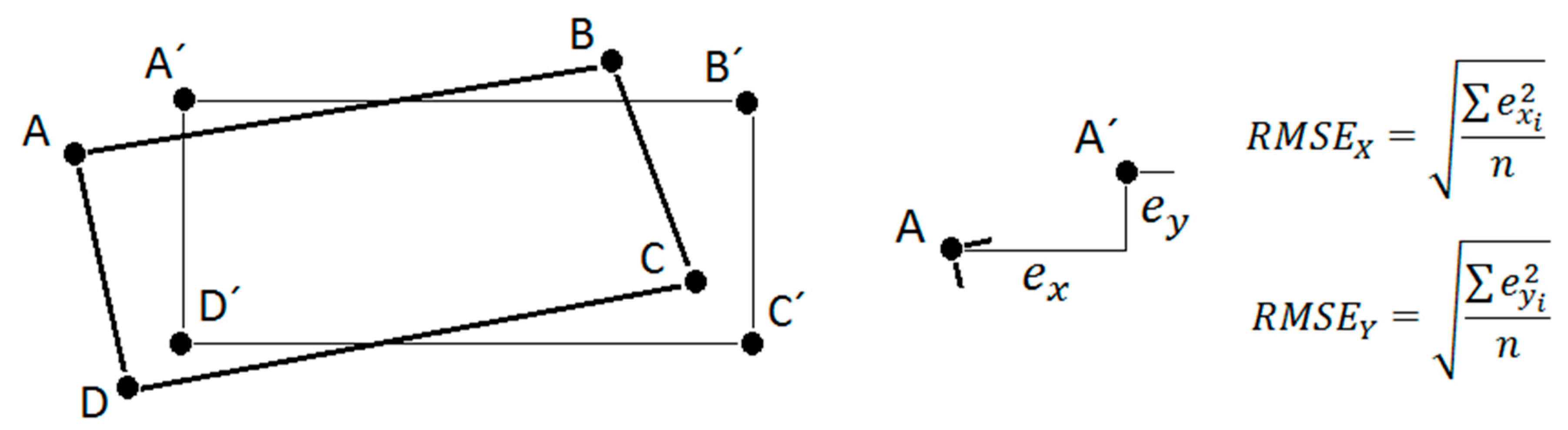
1- Select a sample of a minimum of 20 check points (n> = 20).
2- Compute individual errors for each point i:
e x i = x 10 k i x 25 k i    e y i = y 10 k i y 25 k i
3- Compute RMSE for each component:
R M S E X =   e x i 2 n    R M S E Y =   e y i 2 n
4- Compute the horizontal RMSE using appropriate expression:
 - If R M S E X = R M S E Y then NSSDA (H) = 2.44771/2 R M S E R = 2.4477 ∗ RMSEX
 - If R M S E X R M S E Y and 0.6 < ( R M S E m i n / R M S E m a x ) < 1 then
NSSDA (H) = 2.4477 ∗ 0.5 ∗ (RMSEX + RMSEY)
  Note: If error is normally distributed and independent in each of the x- and y-components, the factor 2.4477 is used to compute horizontal accuracy at the 95% confidence level [25].
Table 3. Mean NSSDA accuracy values and variability obtained.
Sample Size nNSSDA Accuracy (m)Deviation ±(m)Variation ±(%)Sample Size nNSSDA Accuracy (m)Deviation ±(m)Variation ±(%)
1012.2241.49512.210012.6270.6505.1
2012.3921.37611.115012.6350.5454.3
3012.4751.1829.520012.6420.4823.8
4012.5201.0488.425012.6400.4213.3
5012.5520.9787.830012.6550.3422.7
6012.5800.8676.935012.6590.2732.2
7012.5980.7986.340012.6620.2181.7
8012.6100.7475.945012.6620.1611.3
9012.6140.6855.450012.6650.1120.9
Table 4. NSSDA accuracy values according to the number of points selected per polygon.
Points × PolygonTotal PointsAccuracy (m)Points × PolygonTotal PointsAccuracy (m)Points × PolygonTotal PointsAccuracy (m)
1137512.6108290213.01215389013.996
2204712.6719317413.10316394314.102
3218912.69810319213.11617399114.154
4231112.72411336813.55218400914.157
5238912.72912355313.61719404614.160
6267212.77313371113.81220--
7279912.88114378813.833---

