Visualization of Pedestrian Density Dynamics Using Data Extracted from Public Webcams


1
Center for Geospatial Analytics, North Carolina State University, Raleigh, NC 27695, USA
2
Department of Parks, Recreation, and Tourism Management, North Carolina State University, Raleigh, NC 27695, USA
3
Marine, Earth, and Atmospheric Sciences, North Carolina State University, Raleigh, NC 27695, USA
*
Author to whom correspondence should be addressed.
ISPRS Int. J. Geo-Inf. 2019, 8(12), 559; https://0-doi-org.brum.beds.ac.uk/10.3390/ijgi8120559
Submission received: 22 October 2019
/
Revised: 14 November 2019
/
Accepted: 1 December 2019
/
Published: 5 December 2019
(This article belongs to the Special Issue Measuring, Mapping, Modeling, and Visualization of Cities)
Abstract
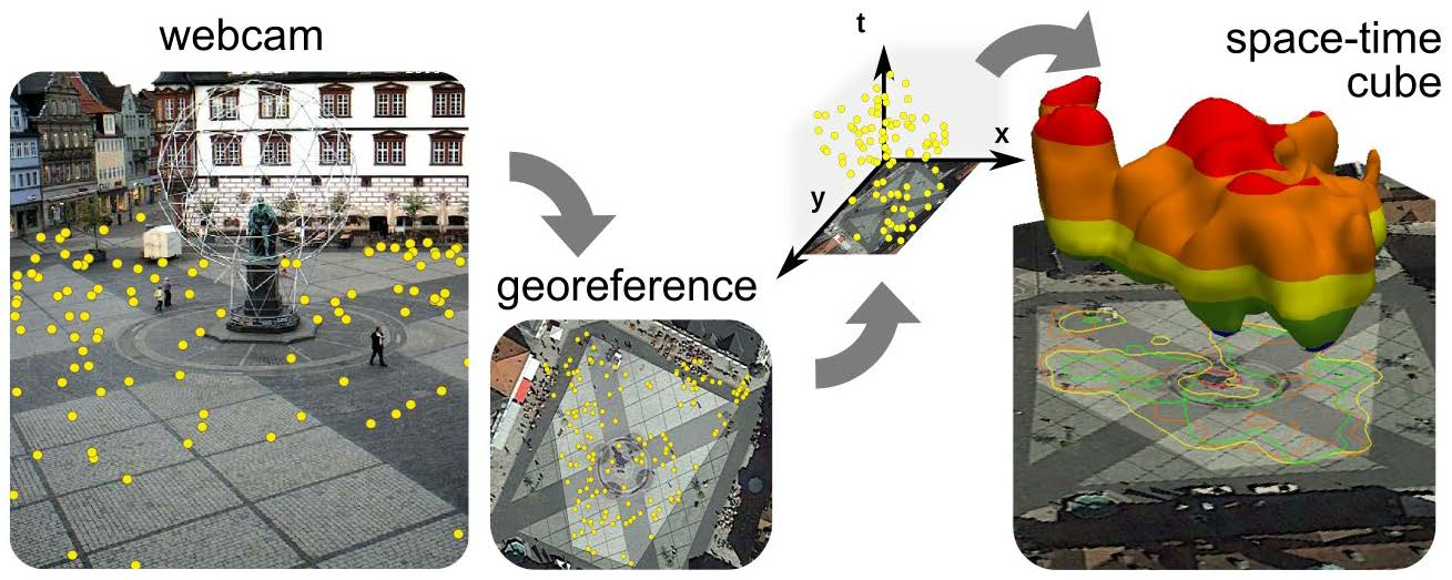
:Accurate information on the number and distribution of pedestrians in space and time helps urban planners maintain current city infrastructure and design better public spaces for local residents and visitors. Previous studies have demonstrated that using webcams together with crowdsourcing platforms to locate pedestrians in the captured images is a promising technique for analyzing pedestrian activity. However, it is challenging to efficiently transform the time series of pedestrian locations in the images to information suitable for geospatial analytics, as well as visualize data in a meaningful way to inform urban design or decision making. In this study, we propose to use a space-time cube (STC) representation of pedestrian data to analyze the spatio-temporal patterns of pedestrians in public spaces. We take advantage of AMOS (The Archive of Many Outdoor Scenes), a large database of images captured by thousands of publicly available, outdoor webcams. We developed a method to obtain georeferenced spatio-temporal data from webcams and to transform them into high-resolution continuous representation of pedestrian densities by combining bivariate kernel density estimation with trivariate, spatio-temporal spline interpolation. We demonstrate our method on two case studies analyzing pedestrian activity of two city plazas. The first case study explores daily and weekly spatio-temporal patterns of pedestrian activity while the second one highlights the differences in pattern before and after plaza’s redevelopment. While STC has already been used to visualize urban dynamics, this is the first study analyzing the evolution of pedestrian density based on crowdsourced time series of pedestrian occurrences captured by webcam images.
Keywords:
GIS; space-time cube; geovisualization; KDE; urban dynamics; georeferencing; pedestrian density
1. Introduction
Understanding the spatio-temporal distribution of pedestrian volume in urban environments is essential for informing urban management and planning decisions to create livable and thriving city centers as well as mitigating negative effects including increased traffic and crime rates. While evidence from public health [1], transportation [2], environmental sciences [3], and environmental psychology [4] can provide theoretical basis for informing urban design, planners are increasingly using data-driven methods to identify opportunities for infrastructure improvements, analyze the use of design features, and evaluate the impacts of special events or public space redevelopment.
Given the importance of up-to-date and reliable data, researchers and urban planners studying the use of public spaces have been testing and applying different types of data collection methods varying in the type and geographic extent of information they provide, cost of their implementation, and privacy issues they raise. Labor-intensive, manual observation methods are often replaced by automated data collection using a variety of technological approaches, such as counting gates, GPS receivers and accelerometers in smart phones [5,6] and more recently also using call detail records (CDR) [7,8] and WiFi probe request data [9]. The challenges of asking people to actively wear the different sensors and privacy issues associated with telecommunication data, together with data and participant inaccessibility for research has led researchers to take advantage of crowdsourced, often publicly available, big data coming from social media networks, such as Twitter, Flickr, and Instagram [10]. Geolocated tweets and images have been used recently to study, e.g., urban parks visitation and access [11,12] and to gain insight about the paths of tourists through cities [13,14]. Strava—a network for tracking athletic activity—provides even more geospatially rich data which has been used to investigate cycling behavior [15], cycling infrastructure [16], and air pollution exposure of commuting cyclists [17].
One of the increasingly popular methods for public space monitoring uses closed-circuit-television (CCTV) footage and webcams to capture and interpret images for a variety of purposes including security, weather monitoring, and pedestrian, bicycle, and motor vehicle traffic [18,19]. Although webcams do not provide individual mobility data, they represent a rich source of spatio-temporal data about people and their environment, and have been used in the past to study air pollution [20], phenology [21], and beach usage [22]. The existing global network of public webcams allows us to study local phenomena on global scale, providing ways to link frequent, high-resolution, on-the-ground observations of environment with typically coarser satellite data [23]. Having recognized the need for an organized, searchable network of webcams, Jacobs et al. [24] established AMOS—Archive of Many Outdoor Scenes—which was collecting images worldwide between 2006 and 2018 and thus capturing the dynamics of urban spaces for many years. As such, AMOS represents a free, unique source of information about pedestrian density, its changes throughout a day, week, month and year, and information on how pedestrians react to changes in their environment. Webcams often capture open places, such as plazas, which typically serve multiple distinct purposes (tourism, commuting, commerce, leisure), and thus other approaches, specifically those gathering data in point locations (e.g., counting gates) or from a specific population (e.g., social networks) may not be effective.
Unlike data from other methods (counting gates, GPS), webcam data cannot be directly analyzed, rather the information—spatial and non-spatial—has to be first extracted, either manually, or automatically using machine learning algorithms, which are increasingly getting better at identifying objects in scenes, whether we look for people, bicycles, or cars. Subsequent spatial analysis typically operates within the coordinate system of the webcam image [18,25], or focuses on pre-defined activity areas [19], limiting the potential of the data to be integrated within existing Geographic Information System (GIS) databases and thus analyzed within the local context. Given the fact that measured distances in webcam images represent varying on-the-ground distances, many urban webcam studies have been focusing on counts and traffic flows rather than spatial mapping [18].
Besides the spatial component of the webcam data, each image is associated with the time when it was captured. Although including the temporal component of the webcam data makes its analysis and visualization much more challenging [26], it provides a more complete picture of the urban dynamics. Space-time cube (STC) representation has proved to be useful means of conceptualization, analysis and visualization of spatio-temporal events [27,28] and trajectories [29]. It has been used for characterizing various urban phenomena, including crime hotspots [30], urban fires [31], and dengue fever [32], as well as for studying human activity patterns [33,34] and describing big trajectory datasets [35,36].
In this paper, we build on a previous study by Hipp et al. [25] and present a new method to derive high-resolution spatio-temporal pedestrian density from webcam images. Given the three-dimensional nature of the density, we propose a novel visualization using a continuous space-time cube representation, aiming at providing at-a-glance view of the dynamics of pedestrian density in space and time. The proposed visualization allows exploration and communication of complex hourly, daily, or weekly spatio-temporal patterns in an efficient and concise way. To demonstrate the method, we analyzed AMOS webcam images capturing two plazas, one in Germany and one in Australia, each highlighting different aspects of the method.
The remainder of the article is organized as follows: in Section 2 we describe data collection and its processing including georeferencing and subsequent aggregation and computation of 2D kernel densities, which are then used to construct the STC representation. Section 3 demonstrates the method using two case studies and summarizes the resulting observations. The strengths and the limitations of the presented method are discussed in Section 4 with conclusion in Section 5.
2. Methodology and Data
2.1. Data Collection
We selected two AMOS webcams, monitoring plazas in Coburg, Germany and Adelaide, Australia, to develop our processing workflows and methodology for computing and visualizing the associated STC representations. Using the metadata information associated with each webcam, we selected the webcam locations and downloaded several months of images which were captured and archived every half an hour. From these images, pedestrian locations were derived using the crowdsourcing platform Amazon Mechanical Turk (MTurk, www.mturk.com). MTurk workers were asked to draw a box around each person found in an image. Each image was annotated by four unique MTurk workers to ensure sufficient reliability [37]; more details about the MTurk data collection can be found in Hipp et al. [25].
To deduplicate the overlapping bounding boxes drawn by multiple workers marking the same person in one image, we averaged the box coordinates when the boxes had overlap greater than 25% and originated from different workers—overlapping boxes by the same worker are likely to be multiple pedestrians close to each other. We converted the deduplicated bounding boxes into a 3D vector point dataset, where each marked rectangular outline of a pedestrian is generalized into an coordinate in the bottom, middle part of the rectangle, representing the pedestrian location. The z coordinate is the time recorded by the annotated webcam image, for our purposes we transformed the image timestamp into the hour of day, ranging from 5 to 21 h (of local time). We did not process images during night due to limitations with visual detection of pedestrians.
2.2. Georeferencing
The marked bounding box of each pedestrian is in the coordinate system of the web camera image. Such representation is not suitable for the analysis of spatio-temporal patterns for multiple reasons. Measured distances in the image coordinate system represent varying distances in reality, hindering the analysis of densities and behavior patterns, e.g., identifying groups versus individuals based on the distance between pedestrians. Furthermore, other relevant geospatial data cannot be simply incorporated into the analysis and visualization. Without transportation networks, amenities, or even modeled cast shadows we may miss proper context of the data, possibly leading to poor understanding of pedestrian behavior.
As with Kako et al. [38], Magome et al. [39], and Willis et al. [40] we used the projective transformation to georeference the pedestrian locations into a projected coordinate system, specifically Universal Transverse Mercator (UTM). For that purpose, we obtained a high-resolution orthoimagery and identified stable features visible in both the orthophoto and the webcam image. In urban environments there is typically enough recognizable features which can be used as ground control points (GCP), including corners of buildings, sidewalks, or monuments, streetlamps, or even colored cobblestone pattern (Figure 1).
Since the captured public squares lie on horizontal planes, we can describe the relation between the webcam image coordinates x, y of the square to the ground coordinates (in the form of homogeneous coordinates , ) using projective transformation:
Ground coordinates can then be computed with:
The coefficients of the homography matrix were estimated from 6 GCPs (minimum is 4 GCPs) using total least-squares method implemented in Python package Scikit-image [41]. To ensure the stability of the computation, we offset the geographic coordinates by subtracting the mean coordinate in x and y directions. The original webcam image and the transformed image are in Figure 1a,b, respectively. Using the same transformation matrix, we transform the pedestrian locations into the ground coordinates using UTM as a coordinate reference system (Figure 1c).
To visualize potential uncertainty coming from imprecisely drawn bounding boxes around pedestrians, we overlaid a grid of circles of 20 px in diameter over the webcam image and reprojected it using the same transformation matrix. Resulting error ellipses in Figure 1c overlaid on top of the orthophoto show how the error changes in shape and magnitude across the observed space. For example, a 5-px error in labeling would result in maximum errors ranging from 0.3 m close to the webcam to 3 m at the far end of the plaza. Greater distance together with acute angle of the webcam cause larger uncertainties, which typically require us to spatially limit the analysis.
2.3. Spatio-Temporal Analysis of Pedestrian Densities
To analyze spatio-temporal patterns of pedestrian distribution we transformed the pedestrian point locations to continuous density representation using bivariate kernel density estimates (KDE) and a space-time cube approach (STC). For further analysis we use only the transformed, ground coordinates in UTM system.
2.3.1. Bivariate Kernel Density Estimate
The estimated pedestrian density can be represented by:
where is the grid point coordinate, is the i-th pedestrian coordinate, n is the total number of pedestrian occurrences, is the Euclidean distance between and , h is the defined bandwidth, is the kernel function, and is the normalized distance . Since KDE has been established as relatively insensitive to choice of kernel function [42], we applied the commonly used bivariate Gaussian kernel function implemented in GRASS GIS v.kernel module [43]:
Selection of bandwidth parameter h controls the level of smoothness of the estimated density. Larger bandwidth highlights statistically stable behavior while smaller bandwidth emphasizes small fluctuations. To estimate the bandwidth, we first tested univariate normal reference rule-of-thumb approach [44] generalized to multivariate setting [42]. Given the observed oversmoothing effect of this approach, we decided to apply maximum likelihood cross-validation method [45], a fully automatic, data-driven method for bandwidth selection implemented in Python package statsmodels [46].
To analyze the variability of daily pedestrian density, we temporally aggregated all pedestrian points from each day of data collection and generated a 2D KDE for each day, resulting in a time series of daily KDE. We then computed the median and interquartile range (IQR) maps for this time series. Similarly, to analyze variability of pedestrian density during a day and during a week we temporally aggregated the points by time of day (ToD) and by day of week (DoW), respectively and computed the ToD KDE and DoW KDE time series. We normalized the resulting KDE time series to compare them. Each KDE in the series was divided by the number of records used for the specific aggregation period (day, time, day of week). For example, for the daily KDE time series, we divided each KDE by the number of captured and processed images for that day.
2.3.2. Space-Time Cube
To visualize the spatio-temporal patterns we represent pedestrian density as a space-time cube (STC), where the x and y axes are in UTM coordinate reference system and the z coordinate is (a) the time of day (ToD), and (b) the day of the week (DoW). We construct STC as a 3D raster, where values are assigned to the center of each voxel (i.e., 3D pixel). We explored several approaches to generating a space-time cube of kernel density estimate. When using trivariate KDE for our type of data, i.e., pedestrian locations at specific times, the trivariate KDE results in spatio-temporal density rates with units number of pedestrians per area and time period. The mapped values are dependent on the frequency of sampling, and thus interpretable only in relative terms. Instead, our STC is constructed from a time series of 2D KDE, representing evolving KDE through time, with units being number of pedestrians per area. To construct such STC it is possible to stack the 2D KDE time series into a voxel model which, in our case, resulted in a fractured representation which was difficult to interpret.
To construct the space-time cube of pedestrian density, which preserves the main features of the space-time pattern while minimizing the noise, we sampled each 2D KDE raster with n points and assigned to these points z coordinates as a) the ToD in hours and b) DoW starting with 0 as Monday. We then used trivariate spline interpolation implemented in GRASS GIS module v.vol.rst [47] to interpolate a 3D raster. Given the sampled points , where p is the number of sampled KDE rasters (e.g., for DoW) the STC representation of can be computed using a trivariate function:
where is the 3D STC grid point coordinate (center of a STC voxel), is the j-th KDE sampled point, is the constant trend, is the interpolation function coefficient, is a tension parameter which controls the range (distance) of influence of the sampled KDE points, is the Euclidean distance between and , is a radial basis function, and . We used radial basis function developed for the regularized spline with tension [47]:
where is the error function. The resulting 3D raster values represent number of pedestrians per area at a location at time z. We performed cross-validation to select optimal parameters of tension and smoothing [47].
The 3D raster representation is advantageous for further analysis, because we can use common raster algebra methods extended to 3D space [48]. 3D rasters of pedestrian density of the same place but for different time periods can thus be compared for example, simply by subtracting one from the other resulting in change 3D raster. Additionally, by extracting values along the time axis at any point in space, for example on sidewalk or near a monument, we can plot and analyze the changing pedestrian density throughout the day.
2.3.3. Space-Time Cube Visualization
As 3D raster representation is commonly used in medicine (such as Computed Tomography scanning), and in some scientific fields such as computational fluid dynamics, there are several common approaches to 3D raster visualization [35], including volume rendering, isosurfaces and slices (Figure 2).
Volume rendering visualizes 3D raster by assigning different color and optical properties to voxels based on their values. Typically, voxels with lower values are rendered as more transparent allowing us to see the structure inside the 3D raster. Volume slices show a cross-section of the 3D raster; usually the 3D raster is sliced in horizontal or vertical direction, but any surface can be used. Isosurface represents a surface joining all 3D points with the same values, and as such it is an equivalent of isoline (i.e., contour line) for 2D surface. The shape of an isosurface of STC KDE shows the spatio-temporal evolution of density, its color is given by the isosurface value. Although it is possible to display multiple isosurfaces at once, interpretation would become very difficult [28]. Often these techniques have interactive components allowing the analyst to manipulate the view to provide additional insights into the properties of the 3D raster.
With any space-time 3D raster visualization rendered on a 2D screen, it is challenging to correctly interpret the relative position of data to axes to accurately answer questions where and when specific event happened [28]. Typically, one needs to manipulate the 3D raster to view it from multiple angles. To make interpretation of 3D space-time pedestrian density easier, we applied technique based on isosurfaces [49], where the time axis is represented as a series of colored bands representing different time intervals draped over the isosurface. This allows a quick understanding of the temporal component without the need for showing a temporal axis, which can be difficult to visually link to 3D raster data (Figure 2). Additionally, we can project slices of the isosurface in the middle of the colored bands on the underlying orthophoto to facilitate the interpretation of spatial patterns. Figure 2d shows an example of such visualization, where each colored stripe represents time interval corresponding to different times of the day, such as morning or afternoon.
2.4. Case Study Data Processing
2.4.1. Marktplatz Coburg, Germany
The processed webcam images in 24-bit sRGB JPEG format were taken every 29 min from 5 to 20 h between 1 May and 31 May 2015, resulting in 478 webcam images and 7417 geolocated pedestrians. We georeferenced the webcam image based on orthoimagery from Google Maps using 6 uniformly distributed GCPs taking advantage of the cobblestone pattern (Figure 1). To increase the reliability of the data we spatially restricted the analyzed area (0.17 ha) to avoid processing points which are too far from the webcam (Figure 1c). The resolution of the webcam (640 × 480 px) can in these cases negatively influence the precision of finding pedestrians and their position. Although the webcam cannot see part of the square behind the statue, this hidden area is relatively small, therefore we decided to not exclude it from the analysis. We selected optimal parameters for KDE bandwidth (2.5 m), sampled KDE series by points and for interpolation we selected tension () and smoothing () for both the ToD and DoW STC. The horizontal resolution of the 2D KDE rasters was 1 m and we multiplied the resulting 3D raster values to represent number of pedestrians per 100 m.
2.4.2. Victoria Square, Adelaide
A sample of available webcam images in 24-bit sRGB JPEG format (Figure 3) from 21 July to 22 September in 2012 (791 geolocated pedestrians in 313 images) and 2014 (2351 geolocated pedestrians in 432 images) were labeled by mTurk workers (with the gap from 8/11 to 8/28 in 2012). Due to the camera resolution (600 × 456 px) we spatially restricted the analyzed area to the northern part of the square (1.15 ha). Upon visual examination of the collected data we observed mTurk workers were consistently confusing certain traffic lights with pedestrians, therefore we removed this part of the data from further analysis, leaving us with 710 and 2284 points for 2012 and 2014, respectively. We selected optimal parameters for KDE bandwidth (6 m), number of sample points and for interpolation tension and smoothing for both years. The horizontal resolution of the 2D KDE maps and STC was 1 m with the resulting 3D raster values then representing number of pedestrians per 100 m.
3. Case Study
The first case study focuses on analysis of spatio-temporal patterns of pedestrian activity during a day and a week. In the second case study we compare the spatio-temporal patterns before and after a plaza redevelopment.
3.1. Marktplatz Coburg, Germany
Coburg is a county-level city with a population of over 40,000 situated in Bavaria, Germany. As an old city dating back to at least the 11th century, Coburg has numerous tourist attractions including Veste Coburg Castle and old town with historically preserved architecture. A public webcam at historic plaza Marktplatz Coburg is oriented approximately in north direction and captures almost the entire square of size 0.56 ha (Figure 1a). The square is dominated by the Prince Albert Memorial in the middle with water fountains around it and there is a permanent fast food stall in the north-east part of the square.
The analysis of the temporal distribution of pedestrians during a day (Figure 4a) reveals highest pedestrian density later in the morning and then in late afternoon, with peaks between 11 and 12 h, and then between 16 and 17 h. The comparison of the number of pedestrians during a week (Figure 4b) shows highest concentrations on Friday and Saturday.
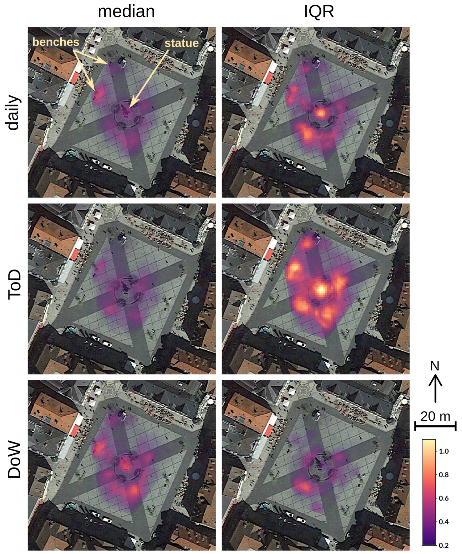
Figure 5 describing the spatial distribution of pedestrians highlights parts of the plaza attracting visitors, including the benches in north-west part of the plaza and areas just below the memorial statue and 10–15 m from the statue in all directions. The comparison of the medians of kernel density estimates based on different temporal aggregations (aggregated by day, time of day, and day of week) shows not all these locations exhibit the same temporal pattern. For example, while the density values around the benches in the west part of the plaza indicate their fairly consistent usage across the aggregation types, the area just below the memorial has higher density values for DoW than for ToD. Focusing on the memorial, the higher median and lower IQR for DoW and the opposite pattern for ToD suggest that the memorial is visited consistently during week but only during peak hours, leaving the space empty for most of the day. Benches are also visited consistently throughout the week, but they are used more consistently throughout the day. Other areas of higher density include areas around the memorial, approximately between 10 to 15 m from it in all directions (except for the north where the memorial was partially obstructing the view). While the variability is generally fairly high across aggregation types, certain parts of the plaza in the south are visited throughout the week and day. Generally higher IQR for ToD densities reflects the fact we take into account peak hours as well as early morning and late evening hours.
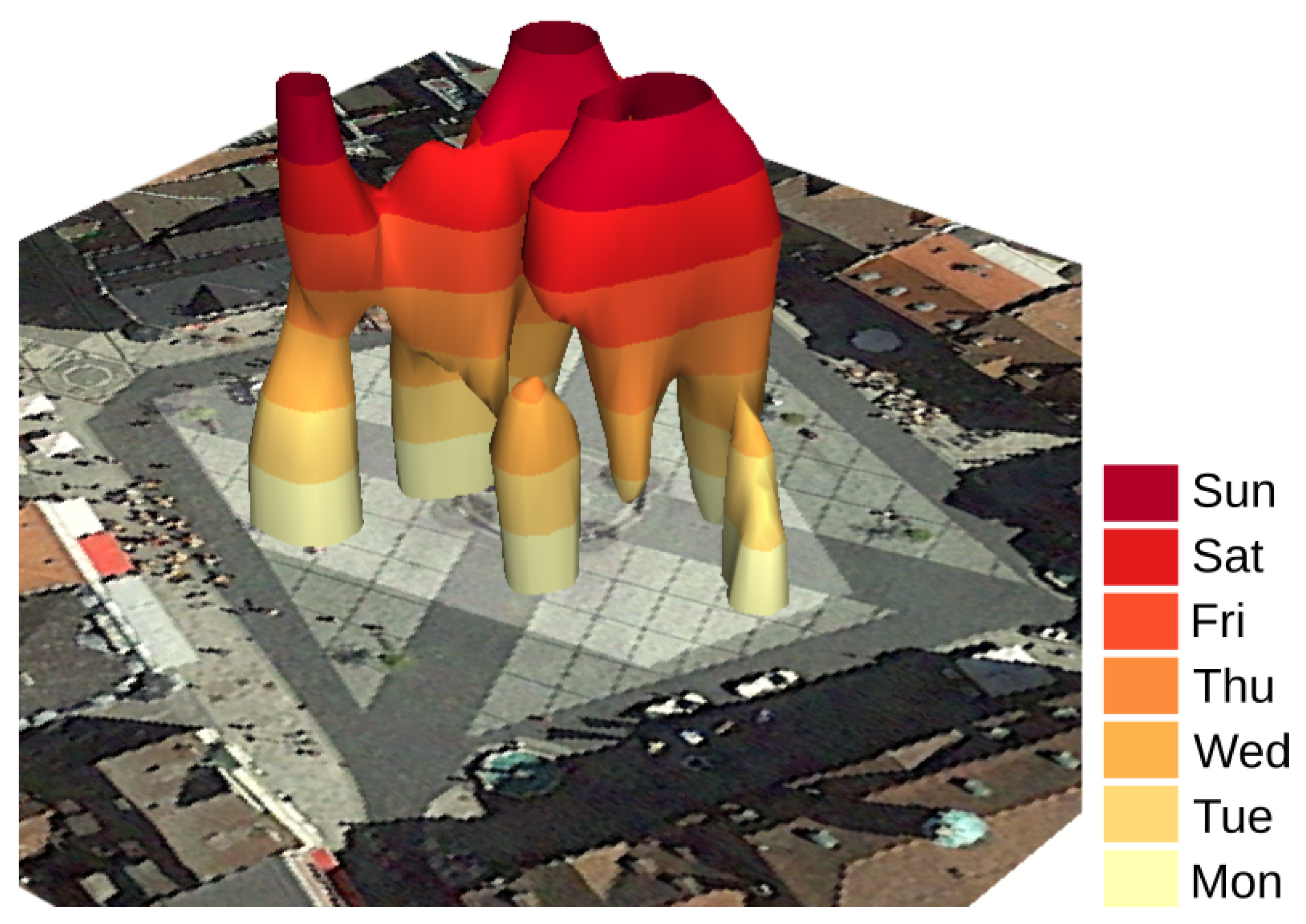
From the ToD and DoW kernel densities we interpolated two 3D rasters of pedestrian densities as they evolve during a day and week, respectively. Figure 6 shows two selected isosurfaces with values 0.5 and 1 pedestrians per 100 m representing medium and high densities, respectively. The funnel-shaped bottom part of the isosurface on the left indicates raising density during the morning, leading to noon and afternoon when most of the plaza is busy. During evening only certain areas around the memorial and benches on the west side of the plaza are being used. The high-density isosurface highlights different patterns for different parts of the plaza. While the south part of the plaza is busiest during noon and the memorial during late afternoon and evening, the benches on the west side are used from noon until evening. The DoW isosurface of 0.5 pedestrians per 100 m in Figure 7 indicates in general higher density in the second part of the week, although certain areas of plaza are busier during the first half of the week. A straight “column” around benches shows they are being used throughout the week.
3.2. Victoria Square, Adelaide
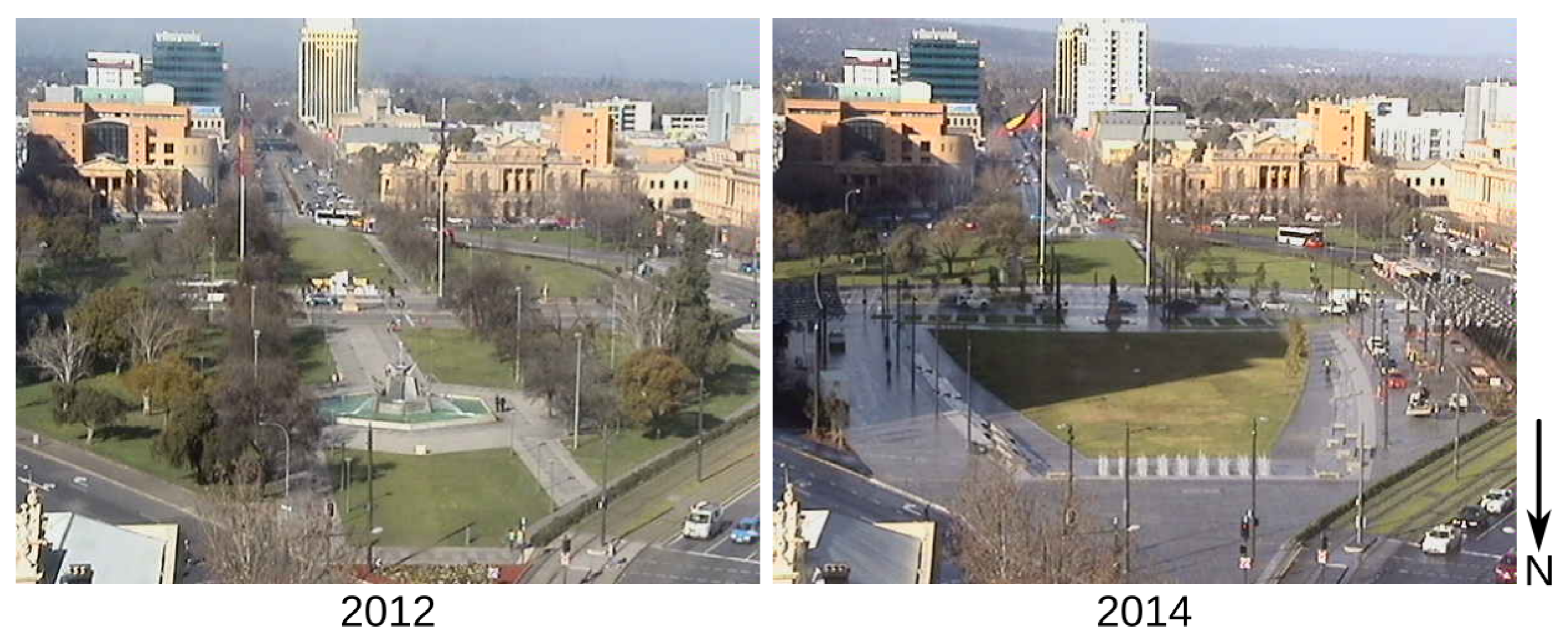
Victoria Square is in the center of Adelaide, the capital of South Australia. Surrounded by a street grid, Victoria Square features a diamond shaped layout with north-south orientation. In 2014 the northern part of the square was redesigned with the goal to create spaces to draw people into the square. Key changes included moving the Queen Victoria statue and relocating the Three Rivers Fountain from north to the square’s southern end, which created space for an outdoor event lawn with an interactive water play area to the north and urban lounges and seating terraces on the sides (Figure 3). The south-facing webcam captured the northern part of the square during the reconstruction, allowing us to analyze the pedestrian density patterns before and after the redesign.
Using median and IQR of ToD-aggregated kernel densities, Figure 8 highlights the similarities and differences between the spatial patterns of pedestrian density before and after plaza’s redevelopment. While the northern part of the plaza has consistently high densities due to the important crosswalk, the densities across the plaza have changed considerably in response to the redevelopment and changes in plaza’s layout. Looking at the magnitude, we can observe higher densities on the paved parts of the plaza after its reconstruction.
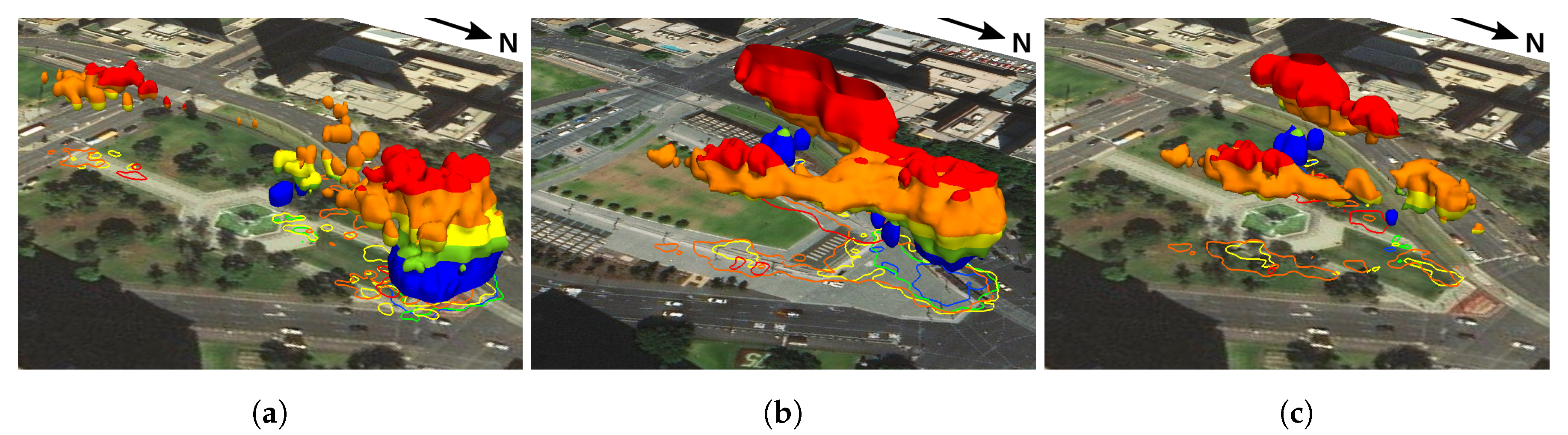
The STC representation in Figure 9 shows the 0.1 density level of pedestrians per 100 m through time of day. The northern part of the plaza was used throughout the day, although after the redevelopment the pedestrian density during morning decreased. The new seating terraces on the sides of the plaza attract visitors mainly during afternoon and evening. The west side has higher densities during early morning and evening. Figure 9c displays the 0.1 isosurface of pedestrian density difference, which we obtain by subtracting 2012 from 2014 density 3D raster. Positive values represent increased density after reconstruction while negative values represent decrease in density. We can see increase in pedestrian density in the afternoon and evening at the sides of the plaza, and in the middle of the day in the northern part where lawn was replaced with paving.
4. Discussion
Collecting data about the use of public spaces and their analysis is instrumental for informing urban design and developing city policies that better reflect the needs of local residents and visitors [8,50]. Increasing walkability, reducing traffic congestion, or identifying underused infrastructure, all these objectives may require different data collection methods and analyses. Moreover, the inherent complexity and spatio-temporal nature of the data calls for effective visualizations to extract meaningful information [29]. In this study, we demonstrated the potential of webcams, an inexpensive and easy-to-use technology to study the current use of public spaces and to evaluate any ongoing changes. We introduced a methodology allowing us to transform time series of webcam images into geospatial representation of pedestrian densities, which can be readily applied to study the current use of public spaces or evaluation of ongoing changes. With the proposed space-time cube representation, we cannot only meaningfully visualize the urban pedestrian dynamics, but also compare space-time cubes derived from different time periods or extract information for specific locations or time instances.
Although this study dealt with pedestrian densities only, it is simple to apply the same method for bicycles or motor vehicles. As with subtracting the space-time cubes before and after reconstruction of the plaza, comparing the space-time cubes representing these different modes of transportation can reveal their interactions, e.g., identify places with safety concerns. Even though the webcam data do not provide information about the direction pedestrians are walking or time spent on one location, we can infer more about the causes of observed patterns by analyzing the densities in the local context including streets, amenities, or current weather. Using Digital Surface Models of cities would enable the incorporation of results from high-resolution spatial modeling of solar radiation or viewscapes [51,52].
Given the growing city sizes and spatial and temporal scarcity of human mobility data, pedestrian volumes have been estimated by simulations, often using agent-based models (ABM) [53]. Given the well-known challenges with calibrating and validating ABMs [40,53,54], deriving pedestrian densities from webcams could replace labor-intensive manual survey methods, especially in open spaces, such as plazas, where ”gate count” methods [55] would be ineffective.
Like other active transportation behavior studies, our methodology includes some limitations and assumptions. Webcams are not always located and oriented in an optimal way. When a webcam is installed low above the terrain, the accuracy of the georeferenced coordinates quickly deteriorates with the increasing distance from the webcam (see the error ellipses in Figure 1). Therefore, the webcam needs to be installed as high as possible to capture areas of interest under large view angles. Furthermore, in this work, we assumed the plazas are perfect horizontal planes, which in many cases is a reasonable assumption. However, in cases where the observed urban area lies on a tilted plane or has even more complex topography, the georeferencing method would need to be corrected to take the topography into account. Finally, obstructions in the webcam view can cause missing data, which may obscure the analysis. This can be a challenge in urban environments with trees or large monuments. A possible solution is to fill the gaps by integrating georeferenced data from a second webcam capturing the area of interest from an alternative location.
Although a crowdsourcing platform has been successfully used before for labeling pedestrians, bikes, and cars [37], in many cases the accuracy may not be sufficient. Requiring multiple workers to repeat the same task may be too costly and it does not necessarily help in avoiding certain issues. For example, with low resolution webcams certain permanent objects may be easily confused with pedestrians. These cases can be fortunately easily detected when looking at the webcam image time series and the affected labels removed. Furthermore, when webcams capture crowded scenes during an event, person labeling the scene will not be able or willing to label everything, leading to likely underestimation of densities. Many of these issues can be solved by using machine learning algorithms to resolve the labeling automatically using the crowdsourced data as a learning dataset. Although not without errors, detection of people in both sparse and crowded images has been studied and successfully used for many years [56,57]. If visibility is reduced due to nighttime, or weather conditions such as heavy rain or fog, the images are most likely unsuitable for analysis. In our case studies we therefore avoided processing night images, but, apart from that we have not encountered any conditions which would significantly affect visibility. To better inform the analysis, future studies may incorporate recorded weather conditions (including rain, temperature, wind) to disentangle the influence of weather on pedestrian density.
Although the pedestrian density could be visualized in a variety of ways the presented space-time cube visualization provides an effective way to communicate the complex information and allows flexibility to explore spatio-temporal patterns based on different temporal aggregation types, where Z axis can represent hours, days, days of the week, or months, depending on the explored patterns. Moreover, STC as a 3D raster data structure can be used for operations such as 3D raster algebra computation or extractions. By time drilling or time cutting [26] we can obtain temporal behavior of density at certain location or spatial density at certain time, respectively. Using 3D raster algebra, we can simply combine different STCs, e.g., representing densities of pedestrian, bikes and cars to analyze when and where there could be a potentially dangerous conflicting use of public spaces. The proposed visualization should be further tested for usability and efficiency, and to identify which audience it is best suited for.
5. Conclusions
This study analyzed the spatio-temporal distribution of pedestrians in public open spaces using crowdsourced data derived from two webcams. Results from the two case studies show that different parts of the plazas have unique, context-specific temporal patterns of pedestrian density within a day and a week. The first case study focused on examining local variations in temporal patterns within a plaza, contrasting places occupied consistently throughout the day and week with places with more time-dependent use. In the second case study, we compare the spatio-temporal patterns of pedestrian density before and after plaza’s reconstruction, leading to completely different spatial pattern and increase in absolute density values.
This study provides a method to obtain georeferenced spatio-temporal data from webcams and proposes the continuous STC representation for its visualization and analysis, leading to novel ways of examining and interpretation of the data. On a local scale, this method allows evaluation of a city’s infrastructure and inform planning decisions, and at the same time—considering the number of public webcams in cities—the proposed approach offers an opportunity to analyze and compare spatio-temporal patterns around the world.
Author Contributions
Conceptualization, A.P., H.M., and J.A.H.; methodology, A.P., H.M.; software, A.P.; validation, A.P.; formal analysis, A.P.; investigation, A.P.; resources, J.A.H.; data curation, A.P., J.A.H.; writing—original draft preparation, A.P.; writing—review and editing, A.P., H.M., J.A.H.; visualization, A.P.; supervision, H.M., J.A.H.; project administration, A.P.; funding acquisition, J.A.H.
Funding
This research received no external funding.
Acknowledgments
We would like to acknowledge Robert Pless and his team for developing and maintaining AMOS infrastructure. We would also like to thank Ladan Ghahramani for helping with data collection.
Conflicts of Interest
The authors declare no conflict of interest.
References
- Handy, S.L.; Boarnet, M.G.; Ewing, R.; Killingsworth, R.E. How the Built Environment Affects Physical Activity: Views from Urban Planning. Am. J. Prev. Med. 2002, 23, 64–73. [Google Scholar] [CrossRef]
- Vuchic, V. Transportation for Livable Cities; Routledge: London, UK, 2017. [Google Scholar]
- Livesley, S.J.; McPherson, G.M.; Calfapietra, C. The Urban Forest and Ecosystem Services: Impacts on Urban Water, Heat, and Pollution Cycles at the Tree, Street, and City Scale. J. Environ. Qual. 2016, 45, 119–124. [Google Scholar] [CrossRef] [PubMed]
- Tabrizian, P.; Baran, P.K.; Smith, W.R.; Meentemeyer, R.K. Exploring perceived restoration potential of urban green enclosure through immersive virtual environments. J. Environ. Psychol. 2018, 55, 99–109. [Google Scholar] [CrossRef]
- Wirz, M.; Franke, T.; Roggen, D.; Mitleton-Kelly, E.; Lukowicz, P.; Tröster, G. Probing crowd density through smartphones in city-scale mass gatherings. EPJ Data Sci. 2013, 2, 1–24. [Google Scholar] [CrossRef] [Green Version]
- Korpilo, S.; Virtanen, T.; Lehvävirta, S. Smartphone GPS tracking—Inexpensive and efficient data collection on recreational movement. Landsc. Urban Plan. 2017, 157, 608–617. [Google Scholar] [CrossRef] [Green Version]
- Yuan, Y.; Raubal, M. Extracting dynamic urban mobility patterns from mobile phone data. In Lecture Notes in Computer Science (Including Subseries Lecture Notes in Artificial Intelligence and Lecture Notes in Bioinformatics); Springer: Berlin/Heidelberg, Germany, 2012; Volume 7478 LNCS, pp. 354–367. [Google Scholar] [CrossRef]
- Calabrese, F.; Diao, M.; Di, G.; Ferreira, J.; Ratti, C. Understanding individual mobility patterns from urban sensing data: A mobile phone trace example. Transp. Res. Part C Emerg. Technol. 2013, 26, 301–313. [Google Scholar] [CrossRef]
- Traunmueller, M.W.; Johnson, N.; Malik, A.; Kontokosta, C.E. Digital footprints: Using WiFi probe and locational data to analyze human mobility trajectories in cities. Comput. Environ. Urban Syst. 2018, 72, 4–12. [Google Scholar] [CrossRef]
- Martí, P.; Serrano-Estrada, L.; Nolasco-Cirugeda, A. Social Media data: Challenges, opportunities and limitations in urban studies. Comput. Environ. Urban Syst. 2019, 74, 161–174. [Google Scholar] [CrossRef]
- Hamstead, Z.A.; Fisher, D.; Ilieva, R.T.; Wood, S.A.; McPhearson, T.; Kremer, P. Geolocated social media as a rapid indicator of park visitation and equitable park access. Comput. Environ. Urban Syst. 2018, 72, 38–50. [Google Scholar] [CrossRef]
- Schwartz, R.; Hochman, N. The Social Media Life of Public Spaces: Reading places Through the Lens of Geotagged Data. In Locative Locative Media; Routledge: New York, NY, USA, 2014; pp. 52–65. [Google Scholar]
- Blat, J.; Fiore, F.D.; Girardin, F.; Ratti, C.; Calabrese, F. Digital Footprinting: Uncovering Tourists with User-Generated Content. IEEE Perv. Comput. 2008, 7, 36–43. [Google Scholar] [CrossRef] [Green Version]
- De Choudhury, M.; Lempel, R.; Yu, C.; Golbandi, N.; Feldman, M.; Amer-Yahia, S. Automatic construction of travel itineraries using social breadcrumbs. In Proceedings of the 21st ACM Conference on Hypertext and Hypermedia, Toronto, ON, Canada, 13–16 June 2010; p. 35. [Google Scholar] [CrossRef]
- Jestico, B.; Nelson, T.; Winters, M. Mapping ridership using crowdsourced cycling data. J. Transp. Geogr. 2016, 52, 90–97. [Google Scholar] [CrossRef] [Green Version]
- Heesch, K.C.; James, B.; Washington, T.L.; Zuniga, K.; Burke, M. Evaluation of the Veloway 1: A natural experiment of new bicycle infrastructure in Brisbane, Australia. J. Transp. Health 2016, 3, 366–376. [Google Scholar] [CrossRef] [Green Version]
- Sun, Y.; Mobasheri, A. Utilizing crowdsourced data for studies of cycling and air pollution exposure: A case study using strava data. Int. J. Environ. Res. Public Health 2017, 14, 274. [Google Scholar] [CrossRef] [PubMed]
- Faro, A.; Giordano, D.; Spampinato, C. Evaluation of the traffic parameters in a metropolitan area by fusing visual perceptions and CNN processing of webcam images. IEEE Trans. Neural Netw. 2008, 19, 1108–1129. [Google Scholar] [CrossRef]
- Placemeter Inc. Placemeter | Quantify the World. 2019. Available online: http://www.placemeter.com (accessed on 3 March 2019).
- Raina, D.S.; Parks, N.J.; Li, W.W.; Gray, R.W.; Dattner, S.L. Innovative monitoring of visibility using digital imaging technology in an arid urban environment. Reg. Glob. Perspect. Haze 2004, 134, 971–990. [Google Scholar]
- Richardson, A.D.; Braswell, B.H.; Hollinger, D.Y.; Jenkins, J.P.; Ollinger, S.V. Near-Surface Remote Sensing of Spatial and Temporal Variation in Canopy Phenology. Ecol. Appl. 2009, 19, 1417–1428. [Google Scholar] [CrossRef]
- Ojeda, E.; Guillén, J.; García-Olivares, A.; Chic, O.; González, R.; Osorio, A. Long-Term Quantification of Beach Users Using Video Monitoring. J. Coast. Res. 2008, 246, 1612–1619. [Google Scholar] [CrossRef]
- Jacobs, N.; Miskell, K.; Pless, R.; Richardson, A.D.; Fridrich, N.; Braswell, B.H.; Burgin, W.; Abrams, A. The global network of outdoor webcams. In Proceedings of the 17th ACM SIGSPATIAL International Conference on Advances in Geographic Information Systems, Seattle, WD, USA, 4–6 November 2009; p. 111. [Google Scholar] [CrossRef]
- Jacobs, N.; Roman, N.; Pless, R. Consistent temporal variations in many outdoor scenes. In Proceedings of the IEEE Computer Society Conference on Computer Vision and Pattern Recognition, Minneapolis, MN, USA, 17–22 June 2007. [Google Scholar] [CrossRef]
- Hipp, J.A.; Manteiga, A.; Burgess, A.; Stylianou, A.; Pless, R. Webcams, Crowdsourcing, and Enhanced Crosswalks: Developing a Novel Method to Analyze Active Transportation. Front. Public Health 2016, 4, 97. [Google Scholar] [CrossRef] [Green Version]
- Bach, B.; Dragicevic, P.; Archambault, D.; Hurter, C.; Carpendale, S. A Descriptive Framework for Temporal Data Visualizations Based on Generalized Space-Time Cubes. Comput. Graph. Forum 2017, 36, 36–61. [Google Scholar] [CrossRef] [Green Version]
- Gatalsky, P.; Andrienko, N.; Andrienko, G. Interactive analysis of event data using space-time cube. In Proceedings of the Eighth IEEE International Conference on Information Visualisation, London, UK, 16 July 2004; pp. 145–152. [Google Scholar] [CrossRef] [Green Version]
- Brunsdon, C.; Corcoran, J.; Higgs, G. Visualising space and time in crime patterns: A comparison of methods. Comput. Environ. Urban Syst. 2007, 31, 52–75. [Google Scholar] [CrossRef]
- He, J.; Chen, H.; Chen, Y.; Tang, X.; Zou, Y. Diverse Visualization Techniques and Methods of Moving-Object-Trajectory Data: A Review. ISPRS Int. J. Geo-Inf. 2019, 8, 63. [Google Scholar] [CrossRef] [Green Version]
- Nakaya, T.; Yano, K. Visualising crime clusters in a space-time cube: An exploratory data-analysis approach using space-time kernel density estimation and scan statistics. Trans. GIS 2010, 14, 223–239. [Google Scholar] [CrossRef]
- Zhang, X.; Yao, J.; Sila-Nowicka, K. Exploring Spatiotemporal Dynamics of Urban Fires: A Case of Nanjing, China. ISPRS Int. J. Geo-Inf. 2018, 7, 7. [Google Scholar] [CrossRef] [Green Version]
- Delmelle, E.; Dony, C.; Casas, I.; Jia, M.; Tang, W. Visualizing the impact of space-time uncertainties on dengue fever patterns. Int. J. Geogr. Inf. Sci. 2014, 28, 1107–1127. [Google Scholar] [CrossRef]
- Kwan, M.P. Interactive geovisualization of activity-travel patterns using three-dimensional geographical information systems: A methodological exploration with a large data set. Transp. Res. Part C 2000, 8, 185–203. [Google Scholar] [CrossRef]
- Kraak, M.j. The Space-Time Cube Revisited from a Geovisualization Perspective. In Proceedings of the 21st International Cartographic Conference (ICC), Durban, South Africa, 10–16 August 2003; pp. 10–16. [Google Scholar]
- Demšar, U.; Virrantaus, K. Space–time density of trajectories: Exploring spatio–temporal patterns in movement data. Int. J. Geogr. Inf. Sci. 2010, 24, 1527–1542. [Google Scholar] [CrossRef]
- Zou, Y.; Chen, Y.; He, J.; Pang, G.; Zhang, K. 4D Time Density of Trajectories: Discovering Spatiotemporal Patterns in Movement Data. ISPRS Int. J. Geo-Inf. 2018, 7, 212. [Google Scholar] [CrossRef] [Green Version]
- Hipp, J.A.; Adlakha, D.; Gernes, R.; Kargol, A.; Pless, R. Do You See What I See: Crowdsource Annotation of Captured Scenes. In Proceedings of the 4th ACM International SenseCam & Pervasive Imaging Conference, SenseCam ’13, San Diego, CA, USA, 18–19 November 2013; pp. 24–25. [Google Scholar] [CrossRef]
- Kako, S.; Isobe, A.; Magome, S. Sequential monitoring of beach litter using webcams. Mar. Pollut. Bull. 2010, 60, 775–779. [Google Scholar] [CrossRef]
- Magome, S.; Yamashita, T.; Kohama, T.; Kaneda, A.; Hayami, Y.; Takahashi, S.; Takeoka, H. Jellyfish patch formation investigated by aerial photography and drifter experiment. J. Oceanogr. 2007, 63, 761–773. [Google Scholar] [CrossRef]
- Willis, A.; Gjersoe, N.; Havard, C.; Kerridge, J.; Kukla, R. Human movement behaviour in urban spaces: Implications for the design and modelling of effective pedestrian environments. Environ. Plan. B Plan. Des. 2004, 31, 805–828. [Google Scholar] [CrossRef] [Green Version]
- van der Walt, S.; Schönberger, J.L.; Nunez-Iglesias, J.; Boulogne, F.; Warner, J.D.; Yager, N.; Gouillart, E.; Yu, T.A. scikit-image: Image processing in Python. PeerJ 2014, 2, e453. [Google Scholar] [CrossRef] [PubMed]
- Li, Q.; Racine, J.S. Nonparametric Econometrics: Theory and Practice; Princeton University Press: Princeton, NJ, USA, 2007; p. 746. [Google Scholar]
- Menegon, S.; Blazek, R. GRASS GIS: v.kernel Module. 2017. Available online: https://grass.osgeo.org/grass76/manuals/v.kernel.html (accessed on 3 March 2019).
- Silverman, B.W. Density Estimation for Statistics and Data Analysis; Chapman & Hall/CRC: Boca Raton, FL, USA, 1986; p. 176. [Google Scholar]
- Duin, R.P.W. On the Choice of Smoothing Parameters for Parzen Estimators of Probability Density Functions. IEEE Trans. Comput. 1976, C-25, 1175–1179. [Google Scholar] [CrossRef]
- Seabold, S.; Perktold, J. Statsmodels: Econometric and statistical modeling with python. In Proceedings of the 9th Python in Science Conference, Austin, TX, USA, 28 June–3 July 2010. [Google Scholar]
- Mitasova, H.; Mitas, L.; Brown, W.; Gerdes, D.P.; Kosinovsky, I.; Baker, T. Modelling spatially and temporally distributed phenomena: New methods and tools for GRASS GIS. Int. J. Geogr. Inf. Syst. 1995, 9, 433–446. [Google Scholar] [CrossRef]
- Petras, V.; Newcomb, D.J.; Mitasova, H. Generalized 3D fragmentation index derived from lidar point clouds. Open Geospatial Data Softw. Stand. 2017, 2, 9. [Google Scholar] [CrossRef] [Green Version]
- Tateosian, L.; Mitasova, H.; Thakur, S.; Hardin, E.; Russ, E.; Blundell, B. Visualizations of coastal terrain time series. Inf. Vis. 2013, 13, 266–282. [Google Scholar] [CrossRef]
- Krizek, K.J.; Handy, S.L.; Forsyth, A. Explaining changes in walking and bicycling behavior: Challenges for transportation research. Environ. Plan. B Plan. Des. 2009, 36, 725–740. [Google Scholar] [CrossRef]
- Li, X.; Ratti, C. Mapping the spatio-temporal distribution of solar radiation within street canyons of Boston using Google Street View panoramas and building height model. Landsc. Urban Plan. 2018. [Google Scholar] [CrossRef]
- Kim, G.; Kim, A.; Kim, Y. A new 3D space syntax metric based on 3D isovist capture in urban space using remote sensing technology. Comput. Environ. Urban Syst. 2019, 74, 74–87. [Google Scholar] [CrossRef]
- Omer, I.; Kaplan, N. Using space syntax and agent-based approaches for modeling pedestrian volume at the urban scale. Comput. Environ. Urban Syst. 2017, 64, 57–67. [Google Scholar] [CrossRef]
- Crooks, A.; Castle, C.; Batty, M. Key challenges in agent-based modelling for geo-spatial simulation. Comput. Environ. Urban Syst. 2008, 32, 417–430. [Google Scholar] [CrossRef] [Green Version]
- Hillier, B.; Penn, A.; Hanson, J.; Grajewski, T.; Xu, J. Natural movement: Or, configuration and attraction in urban pedestrian movement. Environ. Plan. B Plan. Des. 1993, 20, 29–66. [Google Scholar] [CrossRef] [Green Version]
- Dollár, P.; Wojek, C.; Schiele, B.; Perona, P. Pedestrian Detection: The State of the Art. IEEE Trans. Pattern Anal. Mach. Intell. 2012, 34, 743–761. [Google Scholar] [CrossRef] [PubMed]
- Ryan, D.; Denman, S.; Sridharan, S.; Fookes, C. An evaluation of crowd counting methods, features and regression models. Comput. Vis. Image Underst. 2015, 130, 1–17. [Google Scholar] [CrossRef] [Green Version]
Figure 1.
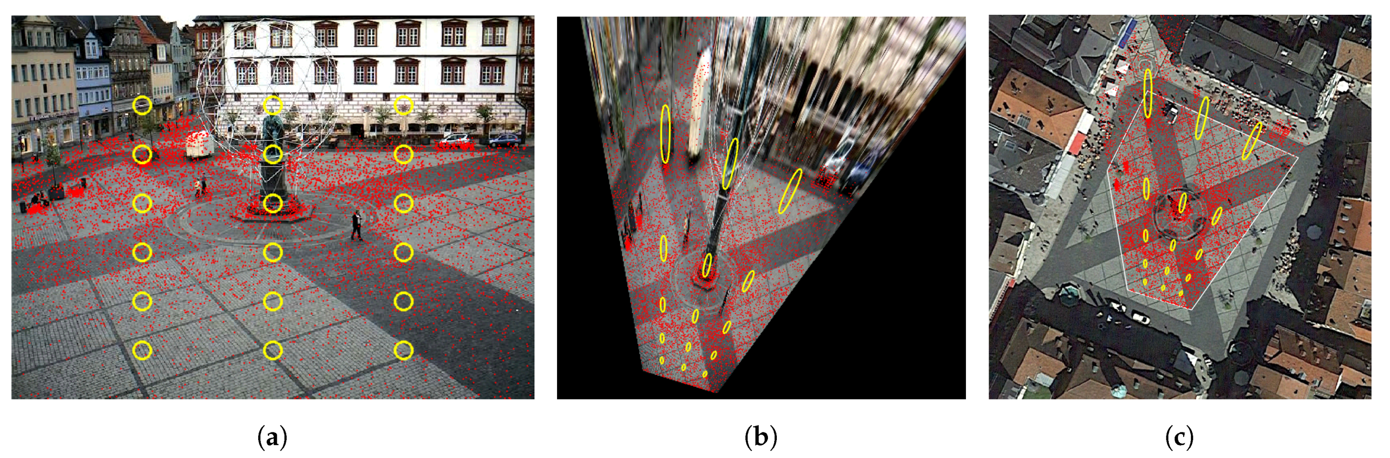
Example of projective transformation of pedestrian locations (red dots) in (a) to UTM coordinates (c) based on orthophoto imagery (Coburg, Germany). The transformed webcam image in (b) is useful for checking the transformation results. Yellow circles in (a) are transformed into error ellipses to map the spatially variable distortions and consequent errors from imprecise labeling of pedestrians. White outline in (c) limits analyzed area.
Figure 1.
Example of projective transformation of pedestrian locations (red dots) in (a) to UTM coordinates (c) based on orthophoto imagery (Coburg, Germany). The transformed webcam image in (b) is useful for checking the transformation results. Yellow circles in (a) are transformed into error ellipses to map the spatially variable distortions and consequent errors from imprecise labeling of pedestrians. White outline in (c) limits analyzed area.

Figure 2.
Examples of 3D raster visualizations: (a) slice, (b) volume rendering, (c) isosurface. Figure (d) shows an isosurface colored based on z-axis with horizontal slices of the isosurface projected on a horizontal plane.
Figure 2.
Examples of 3D raster visualizations: (a) slice, (b) volume rendering, (c) isosurface. Figure (d) shows an isosurface colored based on z-axis with horizontal slices of the isosurface projected on a horizontal plane.

Figure 3.
South-facing webcam capturing images of Victoria Square in Adelaide, Australia, before and after redevelopment.
Figure 3.
South-facing webcam capturing images of Victoria Square in Adelaide, Australia, before and after redevelopment.

Figure 4.
Number of pedestrians observed between May 1st and May 31. Temporal distribution based on: (a) a time of day, and (b) a day of week.
Figure 4.
Number of pedestrians observed between May 1st and May 31. Temporal distribution based on: (a) a time of day, and (b) a day of week.
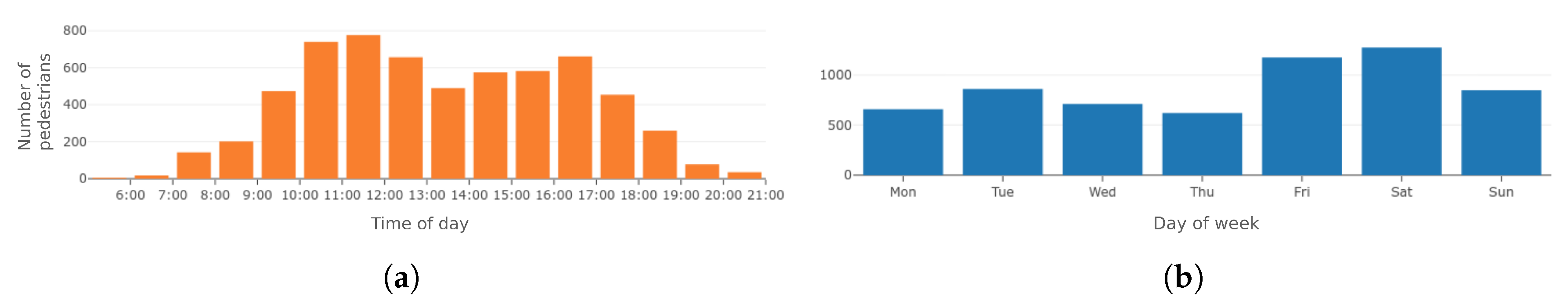
Figure 5.
Median and IQR of number of pedestrians per 100 m at Marktplatz Coburg for different temporal aggregations types: day of week (DoW), time of day (ToD) and daily aggregation.
Figure 5.
Median and IQR of number of pedestrians per 100 m at Marktplatz Coburg for different temporal aggregations types: day of week (DoW), time of day (ToD) and daily aggregation.

Figure 6.
Pedestrian density ToD STC visualization of Marktplatz Coburg using colored isosurface of value (a) 0.5 and (b) 1 pedestrian per 100 m. Highlighted area of the plaza corresponds to the area visible from the webcam.
Figure 6.
Pedestrian density ToD STC visualization of Marktplatz Coburg using colored isosurface of value (a) 0.5 and (b) 1 pedestrian per 100 m. Highlighted area of the plaza corresponds to the area visible from the webcam.
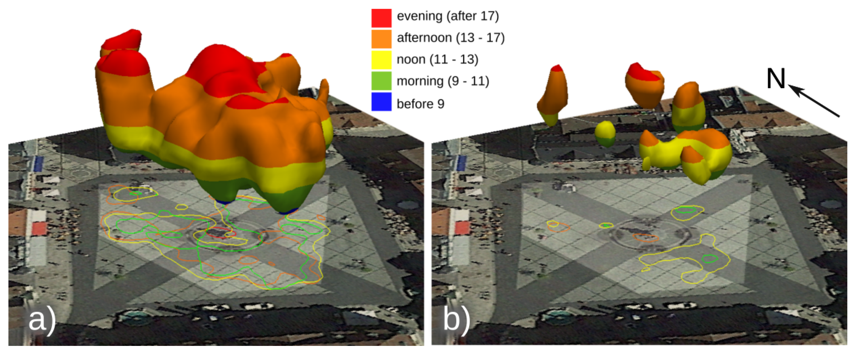
Figure 7.
DoW STC showing isosurface of 0.5 pedestrians per 100 m at Marktplatz Coburg.

Figure 8.
ToD median and IQR of number of pedestrians per 100 m at Victoria Square, Adelaide.
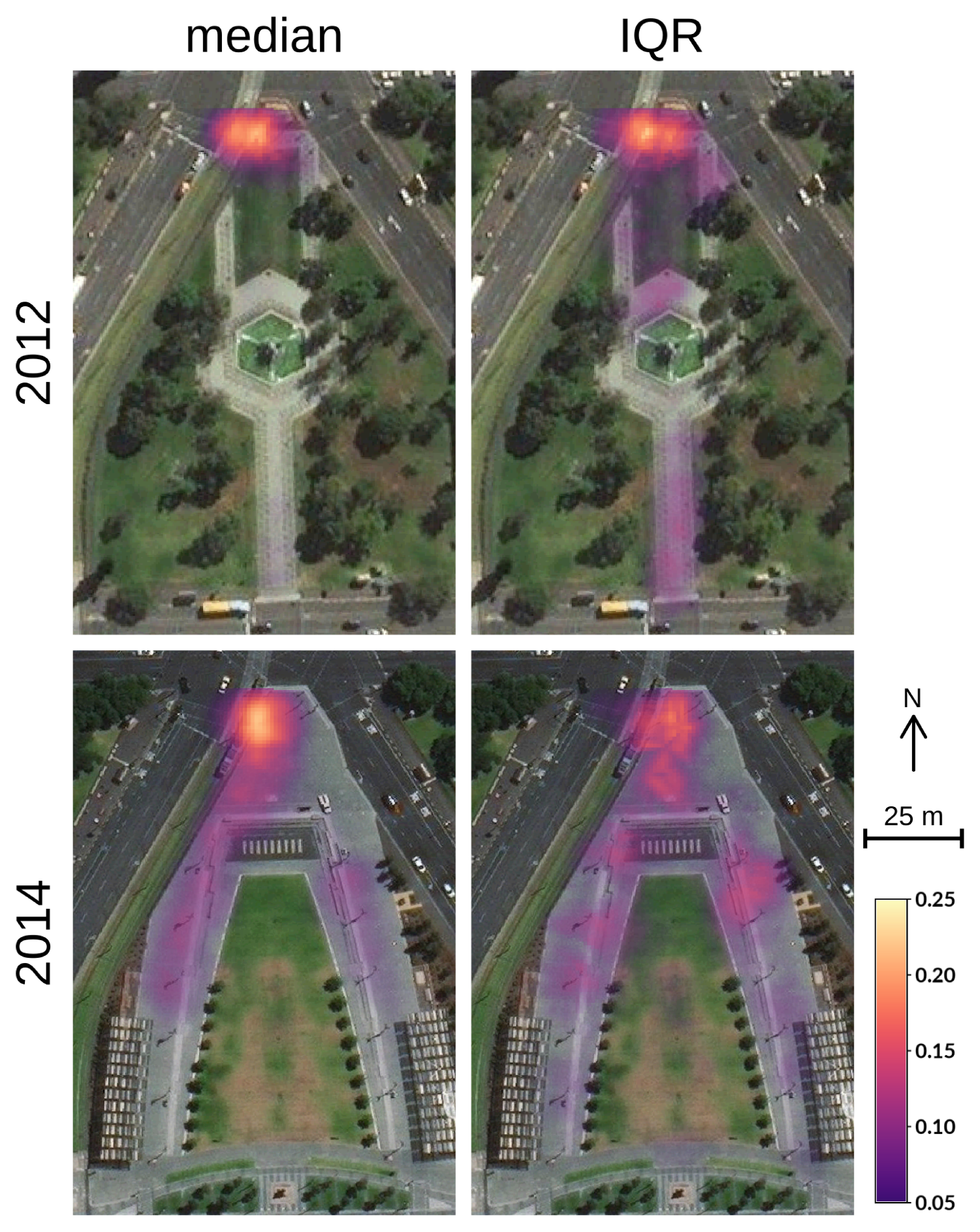
Figure 9.
ToD STC visualization of pedestrian density (0.1 pedestrians per 100 m) (a) before, (b) after Victoria Square reconstruction. Figure (c) shows isosurface of value 0.1 of density difference between 2014 and 2012 representing areas and times with higher pedestrian density in 2014. See Figure 6 for color legend.

© 2019 by the authors. Licensee MDPI, Basel, Switzerland. This article is an open access article distributed under the terms and conditions of the Creative Commons Attribution (CC BY) license (http://creativecommons.org/licenses/by/4.0/).
Share and Cite
MDPI and ACS Style
Petrasova, A.; Hipp, J.A.; Mitasova, H. Visualization of Pedestrian Density Dynamics Using Data Extracted from Public Webcams. ISPRS Int. J. Geo-Inf. 2019, 8, 559. https://0-doi-org.brum.beds.ac.uk/10.3390/ijgi8120559
AMA Style
Petrasova A, Hipp JA, Mitasova H. Visualization of Pedestrian Density Dynamics Using Data Extracted from Public Webcams. ISPRS International Journal of Geo-Information. 2019; 8(12):559. https://0-doi-org.brum.beds.ac.uk/10.3390/ijgi8120559
Chicago/Turabian StylePetrasova, Anna, J. Aaron Hipp, and Helena Mitasova. 2019. "Visualization of Pedestrian Density Dynamics Using Data Extracted from Public Webcams" ISPRS International Journal of Geo-Information 8, no. 12: 559. https://0-doi-org.brum.beds.ac.uk/10.3390/ijgi8120559
Note that from the first issue of 2016, this journal uses article numbers instead of page numbers. See further details here.