A New, Score-Based Multi-Stage Matching Approach for Road Network Conflation in Different Road Patterns


Department of Geomatic Engineering, Faculty of Civil Engineering, Yildiz Technical University, Davutpasa Campus, 34220 Esenler, Istanbul, Turkey
*
Author to whom correspondence should be addressed.
ISPRS Int. J. Geo-Inf. 2019, 8(2), 81; https://0-doi-org.brum.beds.ac.uk/10.3390/ijgi8020081
Submission received: 31 December 2018
/
Revised: 29 January 2019
/
Accepted: 11 February 2019
/
Published: 13 February 2019
(This article belongs to the Special Issue Multi-Source Geoinformation Fusion)
Abstract
:Road-matching processes establish links between multi-sourced road lines representing the same entities in the real world. Several road-matching methods have been developed in the last three decades. The main issue related to this process is selecting the most appropriate method. This selection depends on the data and requires a pre-process (i.e., accuracy assessment). This paper presents a new matching method for roads composed of different patterns. The proposed method matches road lines incrementally (i.e., from the most similar matching to the least similar). In the experimental testing, three road networks in Istanbul, Turkey, which are composed of tree, cellular, and hybrid patterns, provided by the municipality (authority), OpenStreetMap (volunteered), TomTom (private), and Basarsoft (private) were used. The similarity scores were determined using Hausdorff distance, orientation, sinuosity, mean perpendicular distance, mean length of triangle edges, and modified degree of connectivity. While the first four stages determined certain matches with regards to the scores, the last stage determined them with a criterion for overlapping areas among the buffers of the candidates. The results were evaluated with manual matching. According to the precision, recall, and F-value, the proposed method gives satisfactory results on different types of road patterns.
1. Introduction
Map conflation has been a popular research field in geographical information science since the first studies on roads in the 1980s by Lynch and Saalfeld [1], Rosen and Saalfeld [2], Lupien and Moreland [3], and Saalfeld [4]. Its main purpose is to produce better maps from sets of two different maps representing the same entities [1]. Cobb et al. [5] observed the necessities of conflation for three main reasons: (1) updating from one to another, (2) improving positional or attribute accuracy, and (3) containing missing information. Besides, the volume of spatial data is rapidly increasing by means of several sources, including governmental and private agencies, and volunteers. Some of these sources are based on sensors of remote sensing (light detection and ranging (LiDAR), unmanned aerial vehicle (UAV) imagery, internet of things (IoT) sensors). Using these kinds of spatial data requires an integration process that handles geo-information fusion. Fusing data extracts suitable geometric and semantic data from multi-source datasets. Map conflation definition agrees with the traditional definition of data fusion that is commonly used in computer science and remote sensing fields [6].
Map conflation requires relations to be established between the geo-objects (i.e., points, lines, and polygons) of the source maps. The determination of relations between geo-objects is called matching. Most matching approaches have been developed based on lines (roads, boundaries, transportation, streams, etc.). However, some studies have been based on points (buildings, POI, junctions, real-time GPS signals, etc.) [2,4,5], and polygons (buildings, triangles, blocks, parcels, etc.) [7,8,9]. The main reasons that most matching studies have focused on roads are (1) the difficulties in establishing relations between complex representations in road networks (patterns, junctions, roundabouts, dead-ends, etc.), (2) the necessities of data enrichment on navigation datasets, and (3) the increasing amount of road data by volunteered geographic information (VGI) projects such as OpenStreetMap (OSM) [10,11,12,13,14].
In earlier road-matching algorithms, calculations on nodes (rubber-sheet transformation, valence, distance, etc.) were used [2,4,5]. However, the complexity of roads required line-specific approaches. Linear-based approaches involved detailed computations on graphs representing the geometric measures (distance, length, angle, buffer growing, etc.) and topological measures (valence, splitting, etc.) [15,16,17,18,19,20,21,22,23]. Some of the matching approaches were fully automated and also had satisfactory results. On the other hand, Xiong and Sperling [16] proposed a semiautomated method that combines an automated algorithm and an interactive procedure to match road networks. Robust correspondences were established for the nodes, edges, and segments between two networks by using a cluster-based matching process. Using the interactive procedure facilitates checking and correcting missing matches visually. However, the semiautomated part of the method relies on operator control and this requires a great effort during the matching process with a great number of objects. Li and Goodchild [21] proposed an optimization model to match road lines using both geometric and semantic measures, and also affine transformation. They used directed Hausdorff distance to take advantage of the asymmetry of a dissimilarity metric. They also used Hamming distance as a dissimilarity indicator between two feature names. However, the use of semantic information can lead to disruptions during the matching process with data from VGI due to the great number of missing semantic attributes. Furthermore, several approaches such as fuzzy-, agent-, and entropy-based approaches have been proposed to conduct the matching process [24,25,26].
Designing an approach for road-matching requires comprehensive research on the basics of road datasets. Ignoring pattern types or sources of road networks might reduce the accuracy and/or quality of matching results. Yang et al. [27] classified block pattern groups and hierarchically matched the nodes in a road network. Koukoletsos et al. [11] proposed a matching procedure for assessing data completeness of VGI data. They proposed a multi-stage approach to match Ordnance Survey data with OSM road data with regards to both geometric (search distance, orientation, buffering lines) and attribute (text) similarities. Pourabdollah et al. [28] conflated OSM road data with attribute-rich Ordnance Survey data to increase the quality. Moreover, in some cases, if linear-based approaches are inadequate for matching processes, the polygon-based approach by Fan et al. [29] might be useful. They proposed a method that starts with the matching of urban block pairs, then continues matching OSM roads with the edges of urban blocks in authority data.
Since the existing methods were only tested in the study areas presented in their papers, they should not be used directly in a study area that has different characteristics from they tested in. While a matching method gives satisfactory results in a grid-patterned road network, it may not be useful for complex road networks. Choosing the proper method for a different study area requires an accuracy assessment. Firstly, some samples containing randomly selected roads are matched manually by a cartographer or an operator. Then, the chosen method conducts the automatic matching process. Finally, the accuracy and completeness for the chosen method are computed with the matching statistics gathered from the comparison with manual matching. As a result, the global assessment might be inferred by the accuracy and completeness of sample datasets.
This study aimed to develop a new matching method, which is a building block of an overall geo-data fusion mechanism, for roads at a similar level of detail to be used without a preprocess (i.e., manual matching and accuracy assessment). To eliminate the need for a preprocess, the proposed method had to be tested on different types of road patterns. The proposed method is score-based and composed of multiple stages. Furthermore, it is a harmonization of point-, line-, and polygon-based approaches. It requires no semantic data such as road names. In the following section, the study area and datasets with regards to pattern type are described. Then, the similarity indicators, which are the basis of the proposed method, are described (i.e., Hausdorff distance, orientation, sinuosity, mean perpendicular distance, mean length of triangle edges, and modified degree of connectivity) and the proposed method composed of five matching stages (matching with respect to point- and line-based scores in stages 1–4 and polygon-based minimum overlapping area in stage 5) is explained. Section 3 presents the results of the experiment, and Section 4 conducts an evaluation of the results by using precision, recall, and F-value. Section 5 concludes the paper with a discussion of the advantages and disadvantages of the proposed method.
2. Materials and Methods
2.1. Study Area, Road Data, and Road Patterns
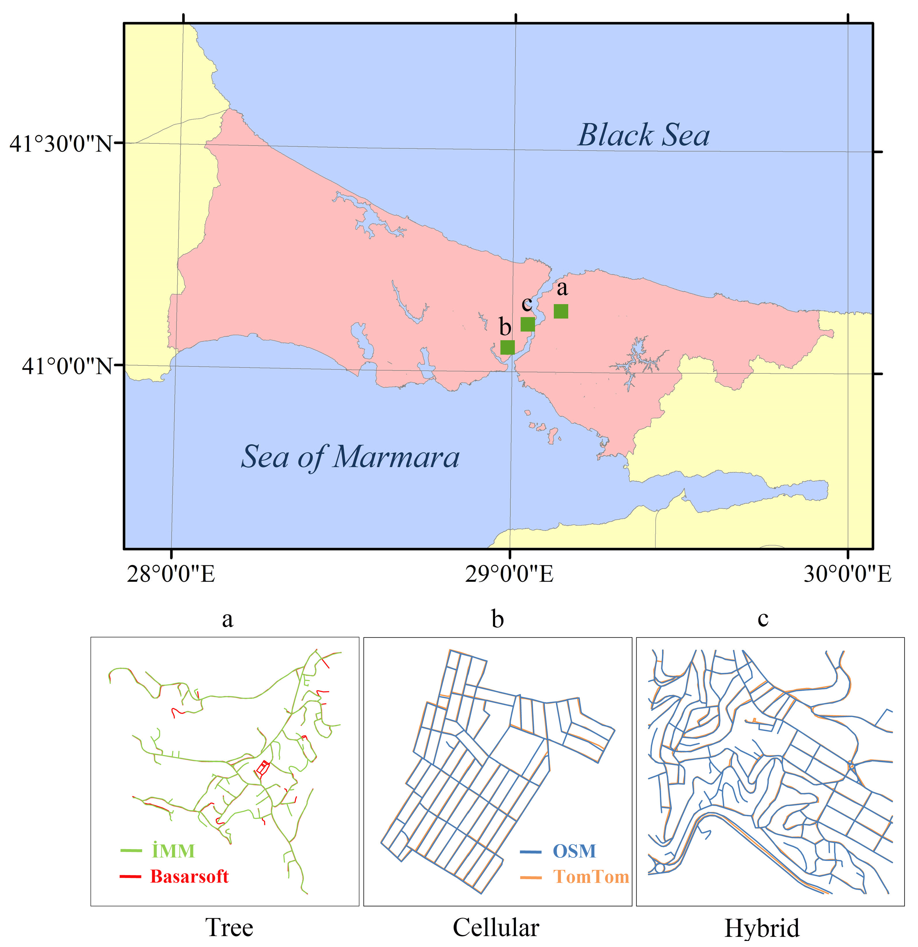
Multi-sourced road networks belonging to the megacity of Istanbul, Turkey were used in this study. The sources are Istanbul Metropolitan Municipality (IMM) (authority), OSM (volunteered), TomTom (navigation), and Basarsoft (navigation). While the authority and private navigation data are topologically structured, OSM data are not. OSM data needs to be topologically structured as well since matching procedures rely on the similarity of road lines.
Marshall’s [30] proposed integrated taxonomy of road patterns distinguishes the road networks generally into five different patterns: linear, tree, radial, cellular, and hybrid. While linear patterns may be part of tree or hybrid patterns, the radial patterns may be composed of a cellular pattern. Therefore, no specific study was conducted on linear and radial patterns. The datasets used in this study are composed of only three distinct patterns: tree (Figure 1a), cellular (Figure 1b), and hybrid (Figure 1c).
2.2. Similarity Measures
Characterizing the road lines into their geometric and topological properties is crucial for matching processes. The properties are the indicators of similarity calculations. The distances, angles, and areas of the shapes are the simple indicators. However, a comprehensive matching algorithm requires more to match differently shaped road lines. The proposed approach uses five geometric and one topological attributes, as described in subsequent sections.
2.2.1. Hausdorff Distance
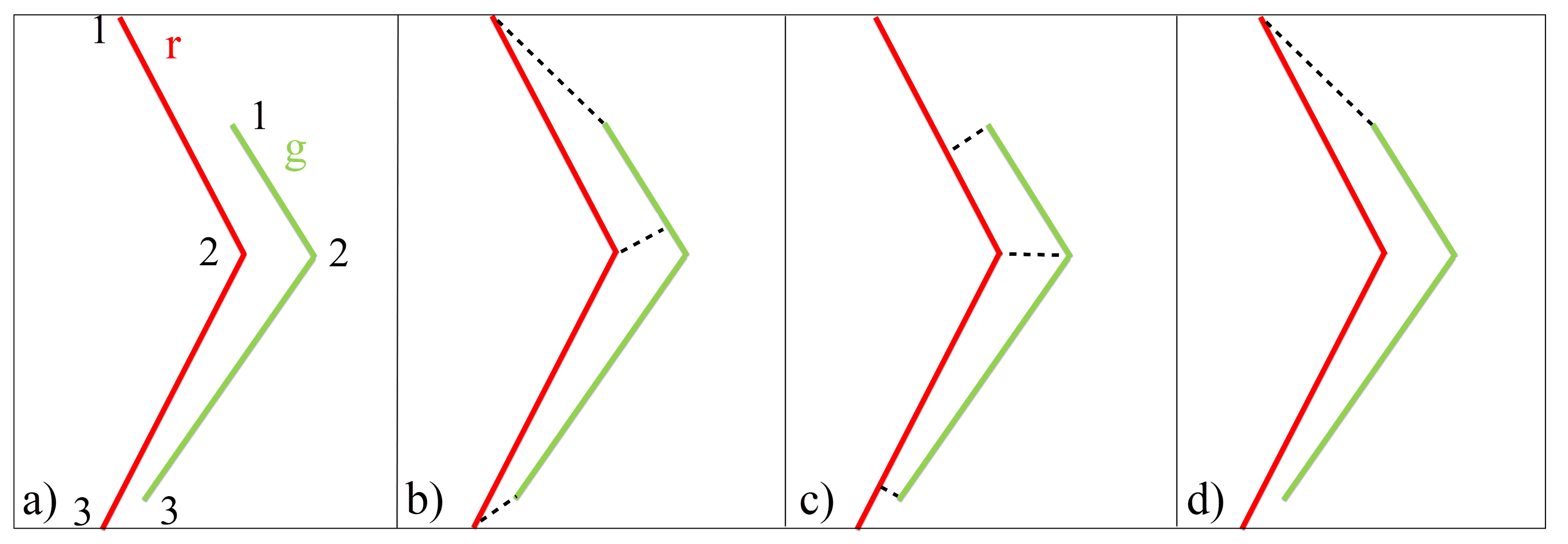
Hausdorff distance is the maximum distance of the minimum distances between two lines or polygons (Equation (1)) [31]. It is used in matching algorithms as a rough selector/eliminator to retain the candidate matching pairs respecting a long threshold that may catch the possible matches. For instance, there are two candidates for matching: Lines r and g (red and green lines in Figure 2a, respectively). The minimum distances from Line r to Line g are (Figure 2b), and the minimum distances from Line g to Line r are (Figure 2c). The maximum distance value in and represents the Hausdorff distance between Line r and Line g. In this case, the asymmetric distance defines the maximum difference between the lines (Figure 2d).
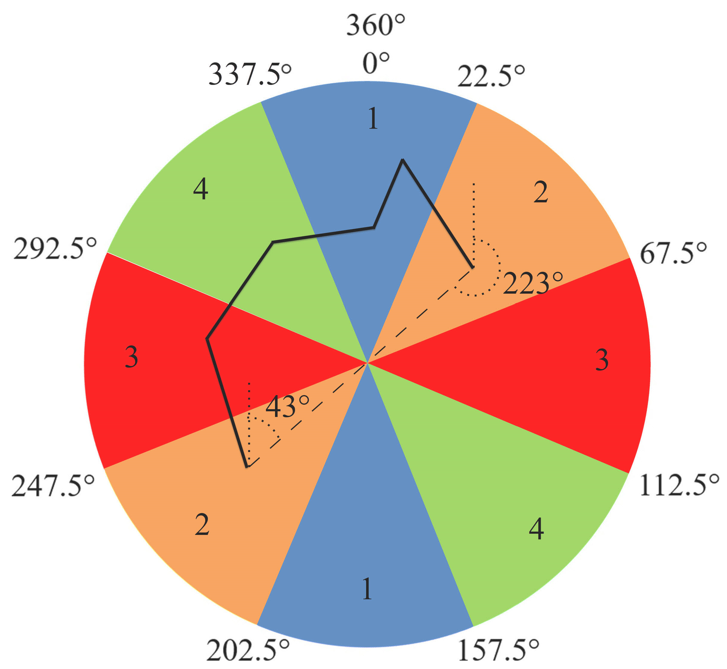
2.2.2. Orientation
Orientation is the rotation angle of the straight line connecting the start and end points of a road line. This indicator facilitates the determination of matching pairs with regard to similar orientations. However, the orientation angle of a line in a dataset cannot be expected to be the same as its certain (correct) matching partner in the other dataset.
Walter and Fritsch [26] mentioned that most of their matching pairs had angle differences of less than 10°, and only a few lines had differences between 10° and 30°. In this paper, instead of only one threshold to determine similar orientations, intervals classifying the orientation differences have been used. A 360° angular system was divided into eight equal orientation intervals (Figure 3).
If two matching candidates are not digitized in the same way (e.g., from left to right), there are approximately 180° of difference between their orientation angles. For instance, if the line in Figure 3 is digitized from left to right, its orientation angle is calculated as 43°. However, if the same line is digitized from right to left, its orientation angle is calculated as 223°. Therefore, the intervals at opposite directions (i.e., the intervals represented by the same color in Figure 3) should be accepted as the same orientation classes. As a result, four orientation classes were used to determine the orientations of the road lines (Table 1). The interval of each class was determined as 45°, which is greater than that of Walter and Fritsch [26] (i.e., 30°), in order to increase the number of possible matches.
2.2.3. Sinuosity
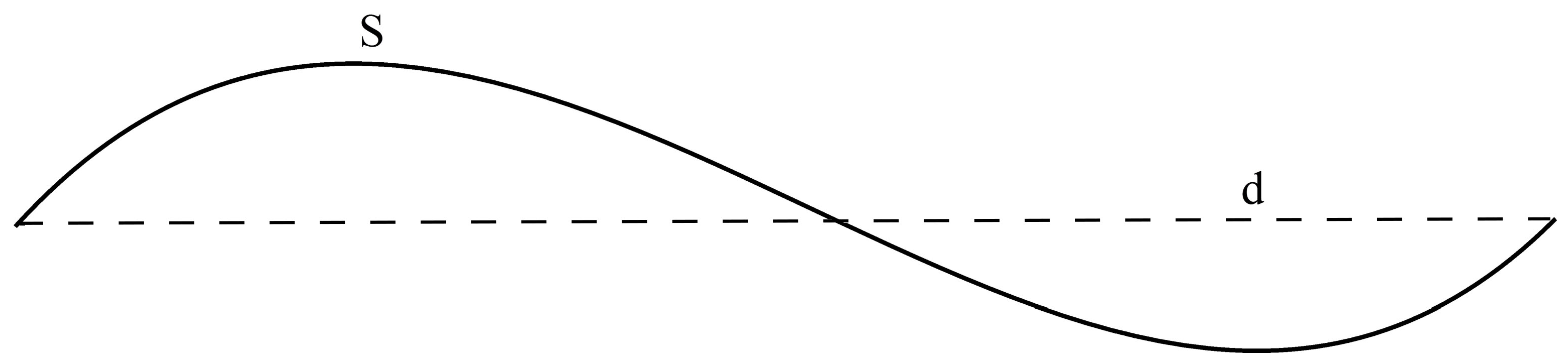
The sinuosity of a road line is the ratio of its sinuous length (e.g., S in Figure 4) to the straight-line distance from its start point to its end point (e.g. d in Figure 4). This measurement defines the curviness of a line [32,33].
Sinuosity indices for road lines are commonly divided into three classes [34]: low (straight and/or low curved roads), middle (relatively curved roads), and high (highly curved roads). In a matching process, the sinuosity index of a road is assumed to be the same as that of its partner. Hacar and Gökgöz [35] determined sinuosity indices with regard to the variations of the sinuosity values of the roads in the source datasets. The maximum variance value of sinuosity () was determined as a threshold in order to calculate the sinuosity intervals. In this study, the sinuosity intervals are used to determine the sinuosity indices (Table 2).
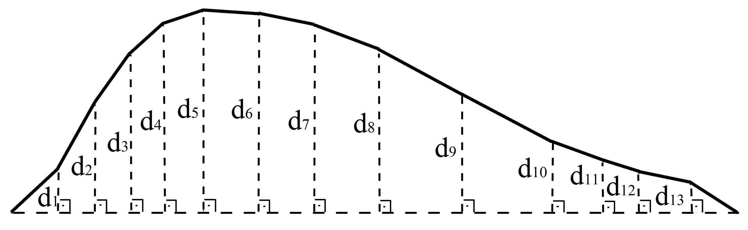
2.2.4. Mean Perpendicular Distance
The mean perpendicular distance is the arithmetic mean of the perpendicular distances from all the mid-vertices of a line to the straight line connecting its start and end points. In Figure 5, (i = 1, 2, …, 13) indicates the perpendicular distances. Equations (2) and (3) compute the perpendicular distances [36] and their arithmetic mean, respectively. A line with long/short mean perpendicular distances is expected to have high/low sinuosity indices, respectively, because they both measure the deviation from the axis of the line (the straight line). Therefore, it can be assumed to be an alternative for or be interoperable with sinuosity indicators.
is the mean perpendicular distance, and are the coordinates of each mid-vertex of a line, and are the coordinates of the start point of the line, and and are the coordinates of the end point of the line.
2.2.5. Mean Length of Triangle Edges
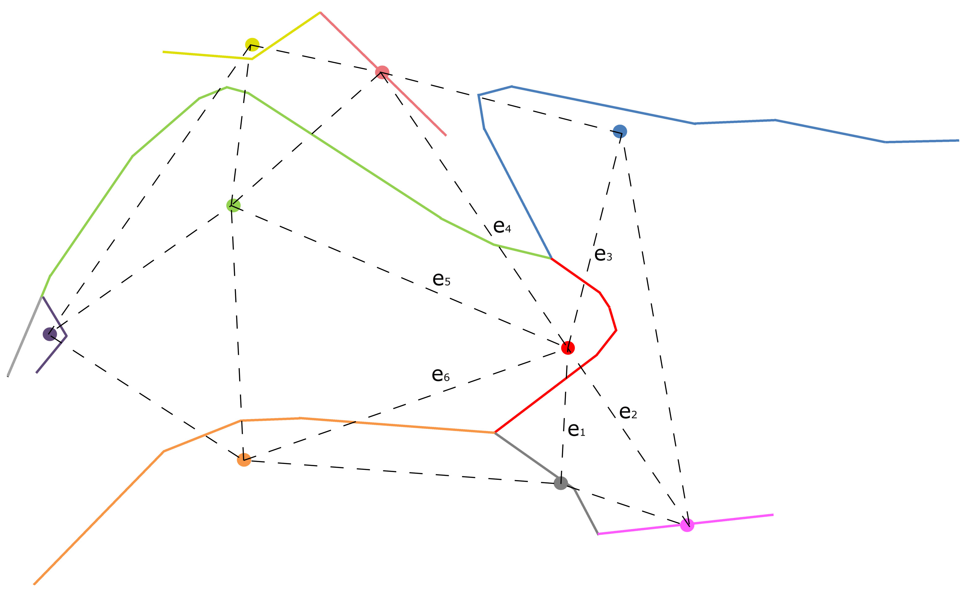
In a matching process, the local proximity of an object to the other objects can also be used. Using the centroid of a line instead of the line is an easy way to compute the local proximity. To conduct the proximity search, a triangulated irregular network (TIN) is generated by using the centroids of road lines [37]. The mean length value of converging triangle edges is computed at related centroids. These values facilitate matching the road lines in different datasets if there is a small difference between the values. Correct matches technically should have similar distances to their own neighbor centroids. From this perspective, this measure can be assumed as a local proximity indicator. For instance, a road line and its centroid are represented by the same color, and the TIN generated by using the centroids of the road lines is represented by dashed lines in Figure 6. Equation (4) computes the mean length of triangle edges ( at a centroid (the red point in Figure 6) as the arithmetic mean of the lengths of the converging edges (e.g., the lengths of the edges (i = 1, 2, …, 6) in Figure 6).
2.2.6. Modified Degree of Connectivity
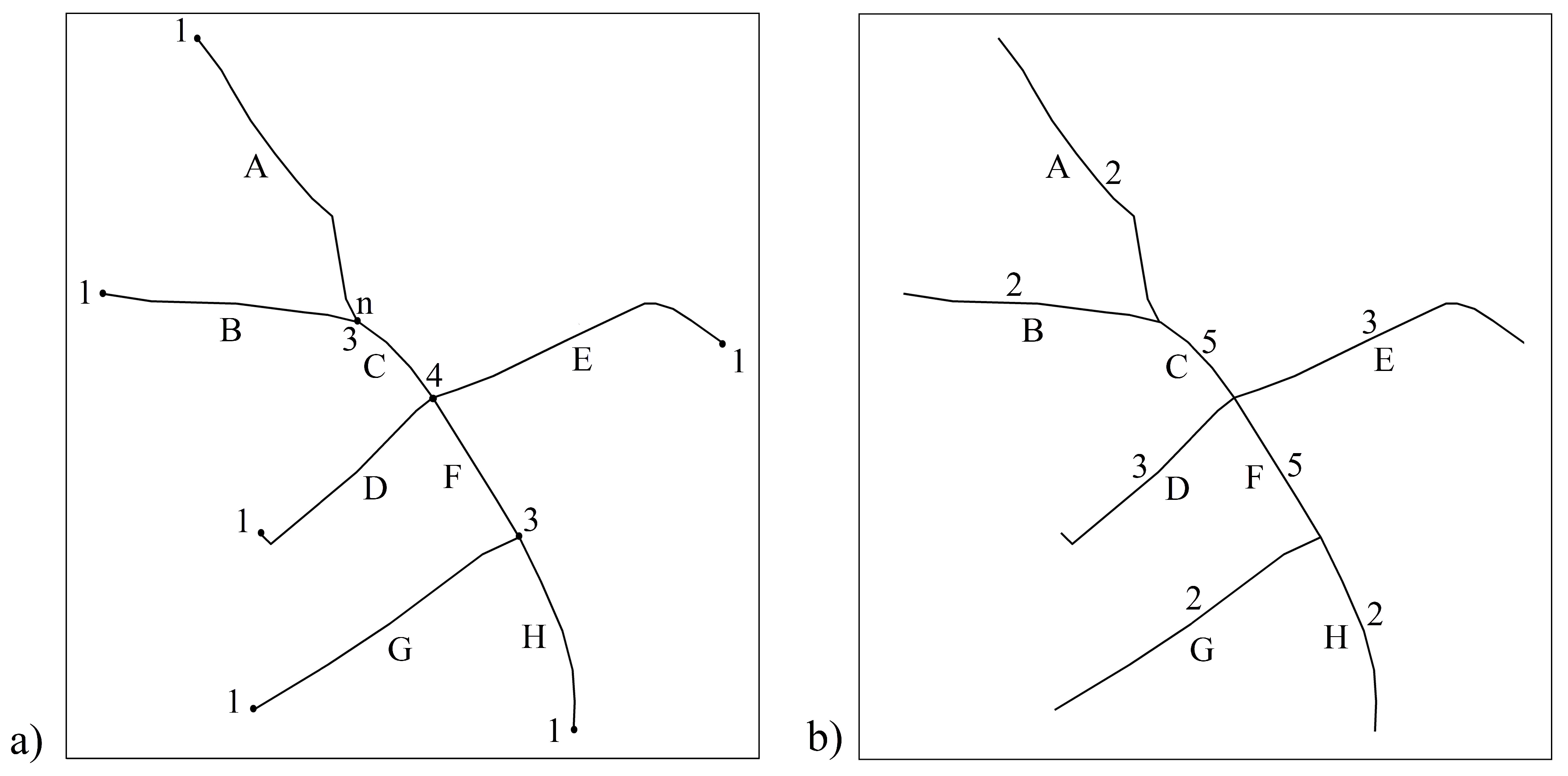
Zhang and Meng [19] and Song et al. [38] used the degree of connectivity (the valence or degree of intersection) as a topological criterion to match candidate pairs. In this study, the modified degree of connectivity facilitates line-to-line matching. Instead of the number of arcs (i.e., road lines) converging to a node, the number of arcs converging to two nodes of an arc is used as the degree of connectivity. For instance, while the degree of connectivity at node n is 3 in Figure 7a, the modified degrees of connectivity of lines A, B, and C (i.e., , and ), which converge to node n, are 2, 2, and 5, respectively, in Figure 7b.
2.3. The Proposed Method: Score-Based Matching
2.3.1. Scores with Respect to the Indicators
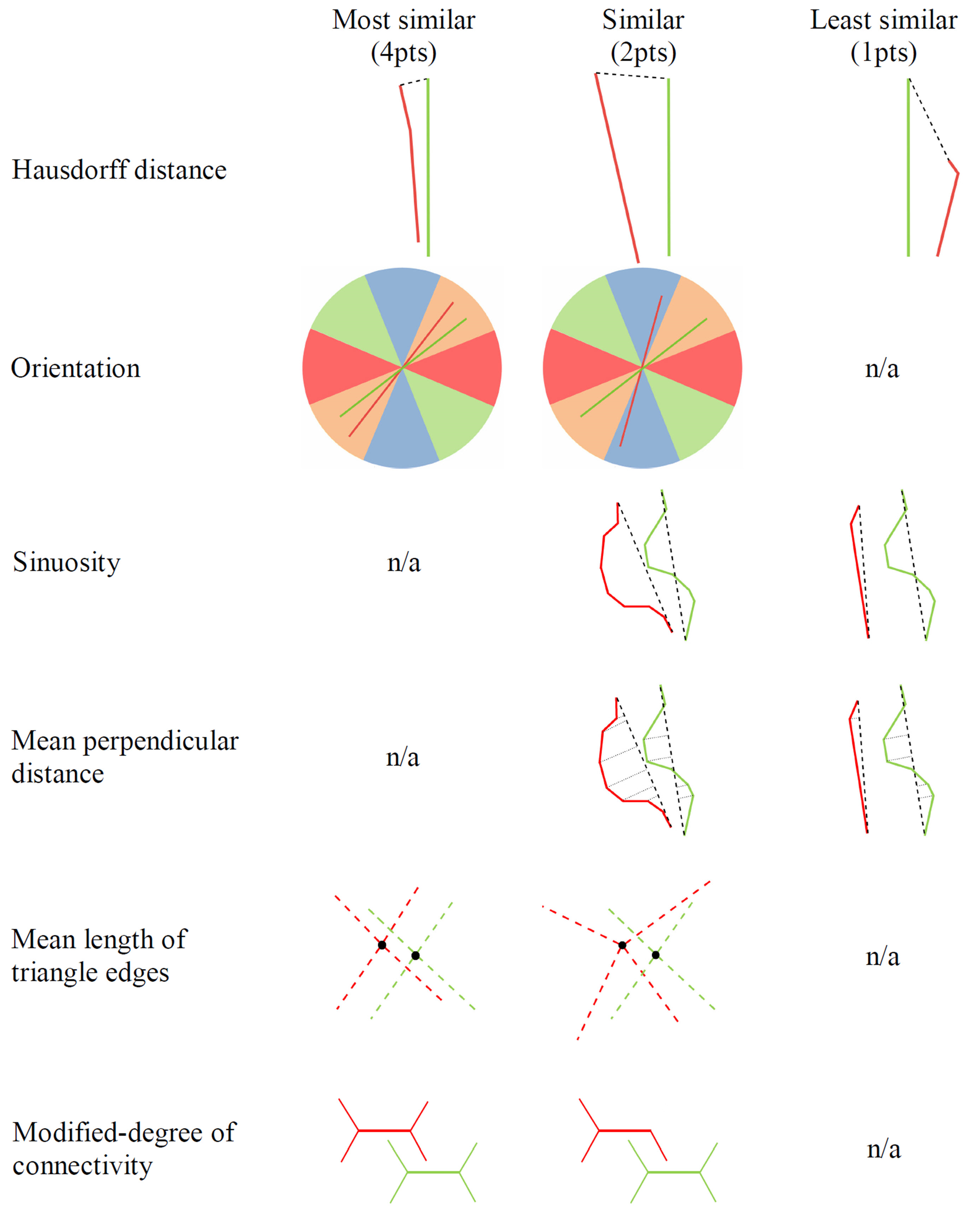
A score describes how candidate pairs are different or similar with respect to an indicator. A general idea of scores is that the most similar candidates have the highest scores. The rules to be considered in determining scores are explained in this section. They are also illustrated in Figure 8. The maximum score to be assigned to a candidate pair with respect to the indicators of Hausdorff distance, orientation, mean length of triangle edges, and modified degree of connectivity is 4. However, since the indicators of sinuosity and mean perpendicular distance represent similar characteristics of road lines, and the maximum score with respect to these indicators is 2, the maximum total score of these indicators shall be the same as the others, 4, for fairness.
- Hausdorff distances from a line to its candidates are sorted ascendingly. The first three of the closest candidate matches are the first three minimum distances between Line n, which is any road line in the first dataset, and Line m, which is the matching candidate of Line n in the other dataset; they are scored as , , and , respectively. If there are more than three candidates, then the fourth and others are scored as .
- The difference between orientation classes where the candidate pair belong ( and ) helps to determine the orientation score (). Candidate pairs in the same class are scored as . If the difference between the classes is one (i.e., if they are in adjacent classes), the score is assigned as . Otherwise, the score is assigned as .
- The rules for sinuosity scores () for Line n in dataset 1 and Line m in dataset 2 are as follows:
- and , then
- and , then
- and , then
- and , then
- and , then
- and , then
- and , then
- and , then
- and , then
- In order to determine the score with respect to mean perpendicular distances, the standard deviation of all mean perpendicular distances () is computed first. If the difference between the mean perpendicular distances of Line n and Line m is less than or equal to , then this matching is scored as . If the difference between the mean perpendicular distances of Line n and Line m is greater than and less than or equal to , then this matching is scored as . Otherwise, this matching is scored as .
- In order to determine the score with respect to the mean length of triangle edges, the standard deviation of all mean lengths of triangle edges () is computed first. If the difference between the mean length of triangle edges of Line n and Line m is less than or equal to , then this matching is scored as . If the difference between the mean length of triangle edges of Line n and Line m is greater than and less than or equal to , then this matching is scored as . Otherwise, this matching is scored as .
- The difference between the modified degree values of Line n and Line m ( and ) helps to determine the score of connectivity. If the candidates have the same degree, then this matching is scored as . If there is a just one degree of difference between the candidates, then this matching is scored as . Otherwise, this matching is scored as .
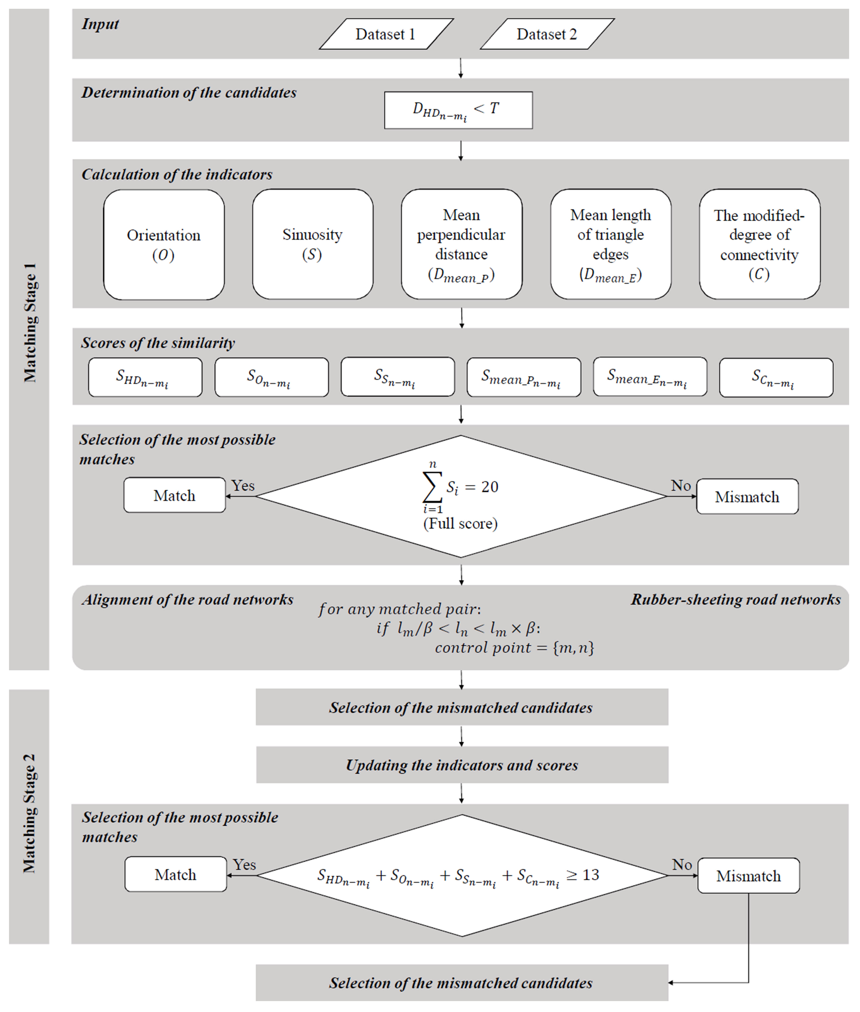
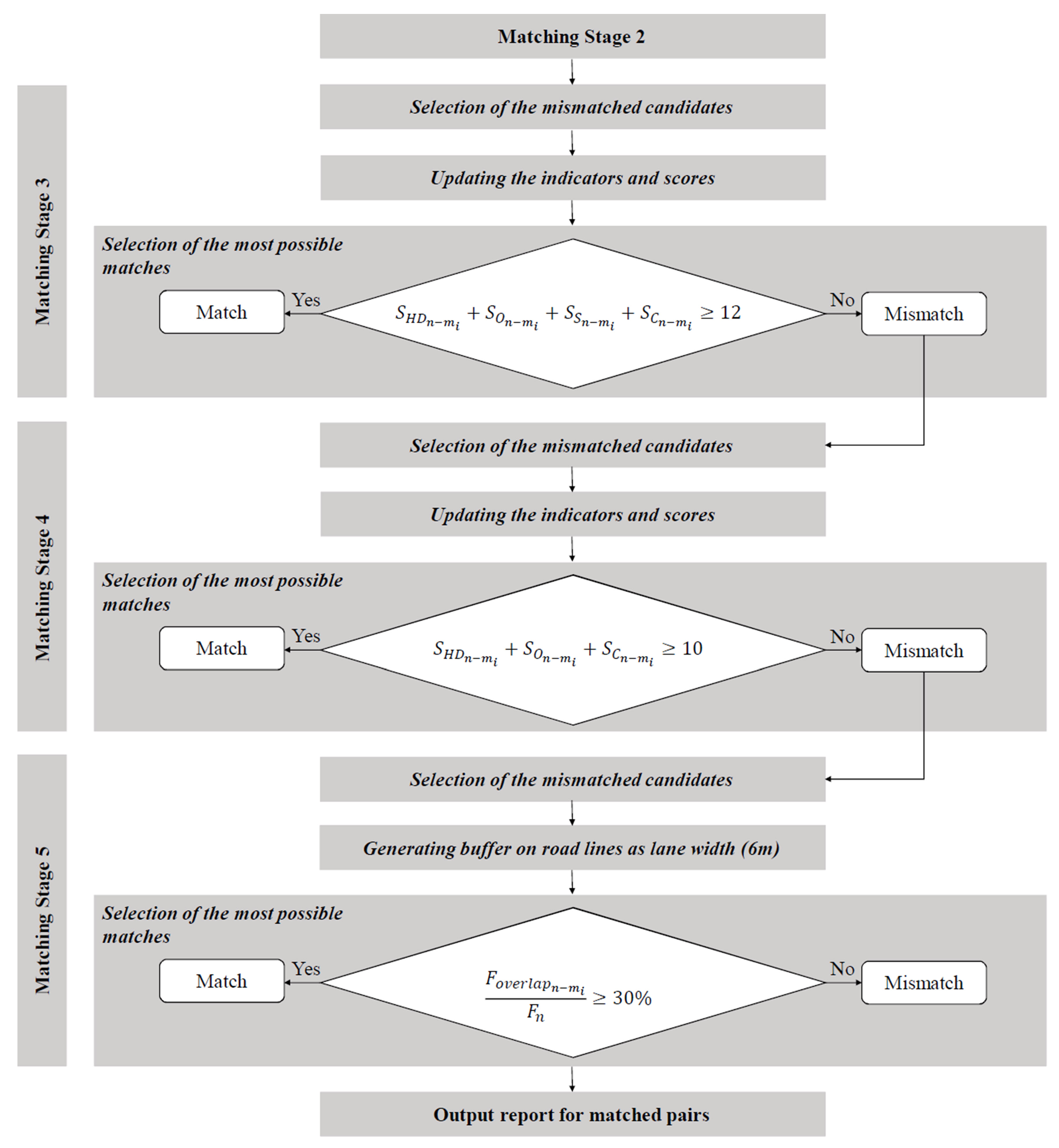
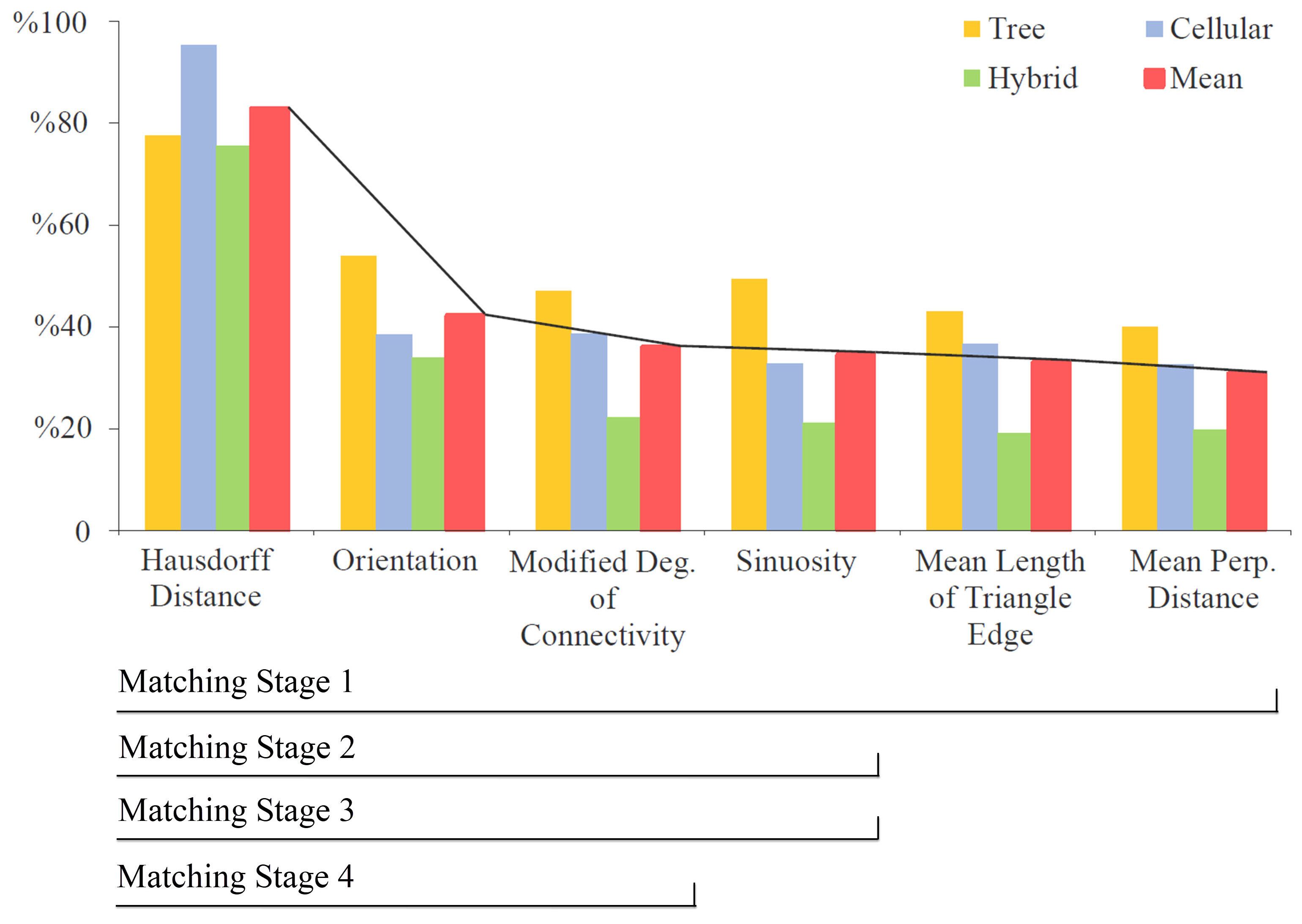
2.3.2. The Stages of the Approach
The proposed approach consists of five matching stages. Each stage has its own matching rules with regards to the scores of the candidates (Figure 9). The matching rules at each stage were determined by using the histogram related to the accuracy distributions of indicators in Figure 10. It was aimed to relax the matching rule some more at each following stage. Therefore, while the less accurate indicators were excluded from the rules, the thresholds for the rules were extended. The first four stages determine some of the certain matches and retain unmatched candidates for the following stage. The fifth stage conducts the last matching, considering overlapping areas.
Matching stage 1: The road lines that are close to each other at less than a pre-defined threshold () are determined as candidate matching pairs. The closeness calculation relies on the Hausdorff distance between each line. Threshold value should be a value by which all possible candidates are determined. The indicators (i.e., orientation class, sinuosity index, mean perpendicular distance, mean length of triangle edges, and modified degree of connectivity) are calculated. The scores of the similarity for each candidate match are computed. The candidate matches that have total scores of 20, in other words, the candidate matches that are the most similar and thus have full scores, are determined as certain matches.
In order to increase similarity, the rubber-sheet transformation aligns the datasets by using the end points of certain matches as control points (Figure 11). However, all of the certain matches are not used. In order to determine certain matches to be used as control points, a tolerance parameter for line similarity proposed by Li and Goodchild [21] is used. The parameter β representing the uncertainty in the length of road lines in different datasets is as follows:
where and are the lengths of Line m and Line n, respectively, and β is the length ratio of all road lines in the datasets. In the proposed approach, this parameter is used to determine the limits of a condition as follows:
According to this condition, if ln is greater than and smaller than , the end points of Line n and Line m are determined as the control points.
Matching stage 2: In this stage, the mean perpendicular distance and the mean length of triangle edges are excluded so that more precise similarity indicators can be considered. The rest of the indicators are updated, and the mismatched candidates are scored. A threshold for the minimum score is considered to determine more certain matches by relaxing the total score. Candidate matches with scores of equal and greater than 13, in other words, the candidate matches that have almost-maximum scores (1 less than the maximum score) are determined as certain matches.
Matching stage 3: The indicators considered in stage 2 are updated for the mismatched candidates, and they are scored. The threshold for the minimum score is reduced to determine more certain matches. Candidate matches with scores of 12 are determined as certain matches.
Matching stage 4: In this stage, sinuosity is also excluded so that more precise similarity indicators can be considered. The indicators (i.e., , ,, , and ) are updated and the mismatched candidates are scored. Candidate matches with scores of 10, in other words, candidate matches that have almost-maximum scores (2 less than the maximum score) are determined as certain matches.
Matching stage 5: Certain matches are determined in accordance with the areas covered by the roads, assuming that each of them is a two-lane road with a width of 6 m (2 lane × 3 m each). The areas are computed using buffers with 6-m widths around the road lines. The ratio of the overlapping area(s) of the two roads to the area of the road in the first dataset is used as a criterion in the following condition:
where is the overlapping area of Line n and Line m and is the area of the buffer of Line n. A candidate pair satisfying this condition is determined as a certain match. At this stage, any Line n and Line m are considered as candidate pair.
This condition is adapted from the study of Fan et al. [29]. In their polygon-based approach, 50% was used as the threshold to match urban blocks. However, since the candidate urban blocks are expected to be more similar than the candidate road areas, the threshold value is reduced to 30% in this study.
3. Results of the Experimental Testing
The experiment was conducted with three differently patterned road networks—tree, cellular, and hybrid—as shown in Figure 1. The thresholds and the number of control points used in the rubber-sheet transformation are given in Table 3. The results of the proposed method were compared to manual matching. As shown in Table 4, the number of missing decreased in each stage. In other words, the cumulative number of correct matches increased in each stage. However, there was no correlation between the numbers of incorrect matches and correct or missing matches. While the maximum number of incorrect matches was seen in the hybrid-patterned network, there were no incorrect matches in the cellular-patterned network.
4. Evaluation of the Results
The results were evaluated in accordance with precision, recall, and F-value, which were computed with Equations (8), (9), and (10) as given by Song et al. [38] and Fan et al. [29]. While precision represents the correctness (accuracy) of the matching, recall (sensitivity) represents completeness. F-value represents the balance between accuracy and completeness. The expectation for the adequacy (sufficiency) of these statistical measures changes relatively in accordance with the aim of the matching process. For instance, while a matching study for navigation datasets is targeted to meet a completeness greater than 85%, the study for a project such as matching passenger or bicycle paths might be expected to be more than 75%. Besides, in a specific matching study, the completeness of the study might be expected to be more precise. For instance, if the source datasets have almost the same number of road lines and also has very similar geometry and topology, the completeness is should a greater value for one-to-one matching.
Correct, incorrect, and mismatch parameters correspond to the true positive, false positive, and false negative, respectively. The mismatch parameter is related to the missing matches, computed as the difference between the number of manually matched pairs and the number of certain matches, composed of correct and incorrect matches.
As shown in Table 5, the most satisfactory results were obtained in accordance with precision representing the accuracy of matching. Since there was no incorrect matching in the cellular-patterned road network (Table 4), the precision of the result was the best of all three network types; a completely correct result was obtained. This was followed by tree- and hybrid-patterned road networks in accordance with their correct and incorrect matchings. Furthermore, with respect to the recall and F-value measures, it seems that the success rating of the proposed method was similar (i.e., cellular followed by tree and hybrid).
The recall values were less than the precision values because of the number of mismatches. The main reason for the higher number of mismatched pairs in the tree- and hybrid-patterned networks is that they are complex, irregular networks, and so the ambiguity between the shapes of the candidates in these networks is more pronounced than in the more regular cellular-patterned road networks.
If the total length of roads in a dataset is relatively similar to the total length of roads in the other dataset, the value of will be close to 1. Otherwise, it is further away from 1. This reflects the similarity of the road networks and can be used as an additional measure in the evaluation of the results. values closer to 1 may indicate more similar road networks. As a result, the order of values computed for each pattern (i.e., 1.02218, 1.06612, and 1.11479 for cellular, tree, and hybrid, respectively) is similar to the order of the networks with respect to the main evaluation measures.
The proposed method is incremental. The matching condition becomes more relaxed in each stage. Therefore, the number of correct matches increases. For example, while the number of correctly matched roads in tree-patterned road networks was 42 in the first stage, 22 road pairs were added in the second stage. On the other hand, the relaxation on the threshold for the minimum score decreased the accuracy. For example, while the accuracy was 100% in the first stage, it was 91.7% in the second stage. This is because the rest of the candidates were less similar than the certain matches in the first stage. Besides, since the indicators used in the fourth stage of the hybrid-patterned road network were not sufficient to match the candidates correctly, the reduction of accuracy was high. None of the other study areas gave such a reduced result in this stage. It can be inferred that sinuosity was a fundamental indicator for the fourth stage of the hybrid-patterned road network.
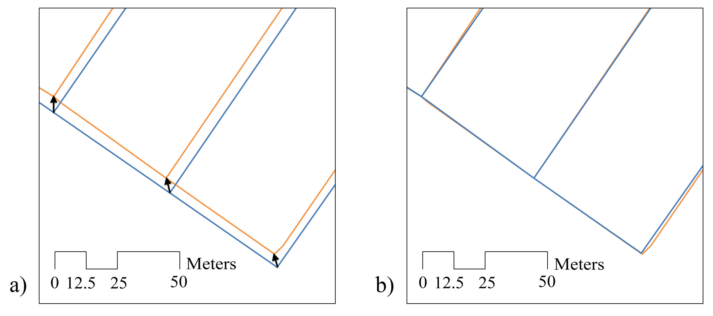
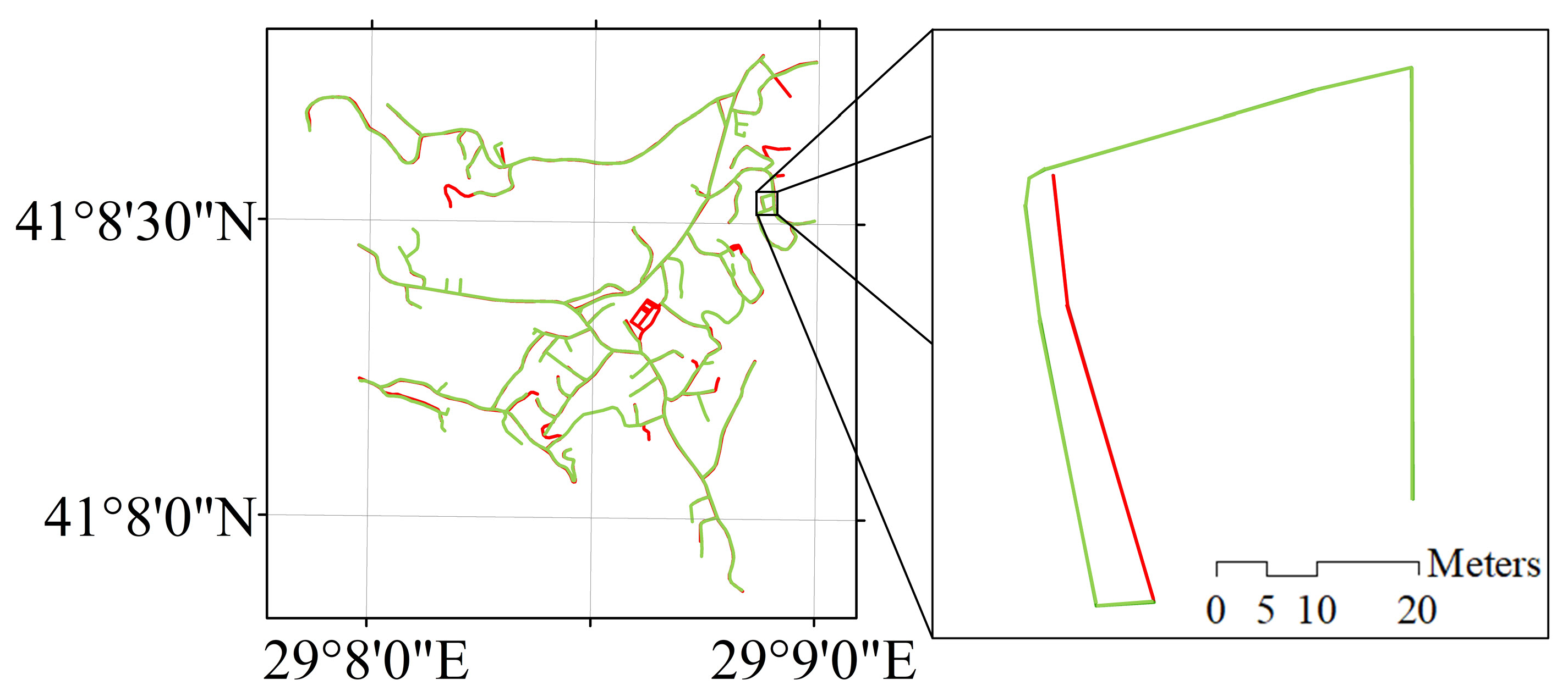
The total number of mismatches in the tree-patterned network was 14. This is mainly because the shapes of the candidates were quite different, as shown in Figure 12. Splitting the longer road lines to match the shorter ones can be a solution for this kind of problem [23].
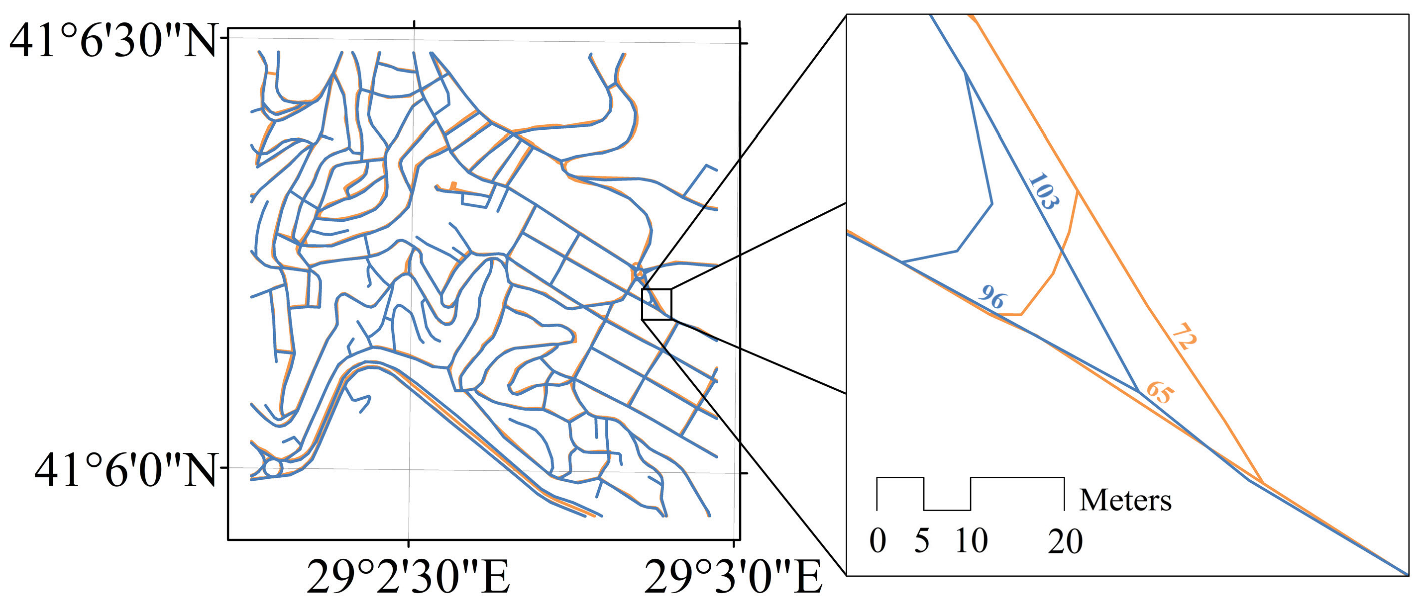
The matching accuracy mainly depends on the number of incorrect matches caused by (1) the indicators, which were not able to measure the similarity, and/or (2) the similarity of the different roads in shape (i.e., geometrically and topologically). For example, Line 103 should be matched one-to-one with Line 72 in Figure 13. However, Line 103 was matched one-to-many with Line 72 (correct) and Line 65 (incorrect). It seems that the incorrect matching of the lines is because Line 103 and Line 65 have similar geometries and topologies. Almost all of these kinds of incorrect matches occurred at specific parts of networks such as roundabouts, junctions, and crossroads. Furthermore, they are generally quite small roads. Matching these kinds of small roads requires additional efforts to reduce the number of incorrect matches.
Experimental Results and Evaluation on Large Datasets
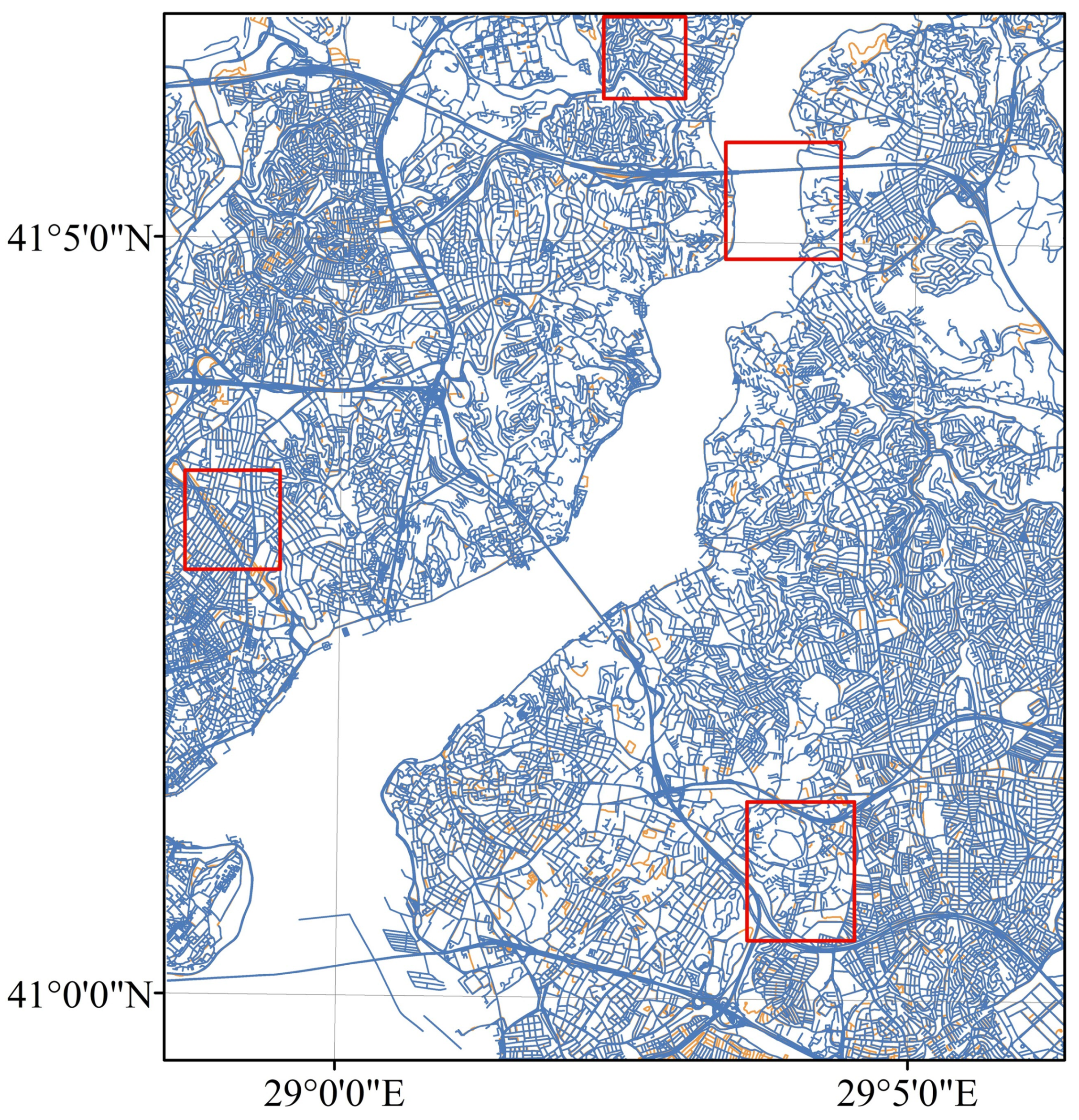
Conducting a global evaluation is a labor-intensive study since manual matching must be conducted by a cartographer (operator), Testing on millions of road segments is not an easy task. In other words, the accuracy of the proposed method on large datasets can only be estimated by weighting the accuracy of samples, which are located on different sides of data extent. As a result, a new matching process has been conducted with large datasets. The road data covers 11 km × 13 km area, in Bosphorus, Istanbul. In these datasets, while OSM has 42264 road lines, TomTom has 29816 road lines. The statistical result of the matching study was computed by comparing the road lines of samples in Figure 14 to manual matchings. The proposed method had a weighted correctness of 91.1%, and this rate also confirms the results on different-patterned road networks.
5. Conclusions
The increase in the production of road data makes it necessary to establish relations between road lines for matching processes. Road-matching requires several preprocess steps such as manual matching and accuracy assessment before its application on multi-source datasets. To prove its efficiency and eliminate the need for preprocesses, the proposed method has been tested on different types of road patterns. It seems that the proposed method has several advantages. It uses point-, line-, and polygon-based indicators together. Some of these indicators (i.e., orientation class, mean perpendicular distance, mean length of triangle edges, and modified degree of connectivity) are presented for the first time in this study. They measure both geometric and topological similarity for matching processes. With the adapted β parameter [21], rubber-sheet transformation is conducted based on certain matching pairs so that the road networks are aligned as correct as possible. The overlapping area [29] are also adapted in the matching procedure to increase the number of correct matches in the last stage. The accuracy is high in each type of road pattern with regards to the evaluation of the precision measure. The proposed method provides excellent results in cellular-patterned road networks. The completeness in each type of road pattern is relatively adequate with regard to the purpose of the matching process.
The results prove that the proposed score-based multi-stage matching method can be used with the road data from authority, private sectors, and volunteers. The proposed method uses no semantic data such as road names and so it is even capable of matching road lines of which names are unknown. It can also be used in tree-, cellular-, and hybrid-patterned road networks.
The proposed method results in more missing matches in irregular road networks (tree- and hybrid-patterned) than that of regular road networks (cellular). Besides, since the similarity indicators mostly determine the main properties of road lines, matching the road lines at specific parts of networks such as roundabouts, junctions, and crossroads correctly is difficult. The proposed method also experienced difficulties when matching longer road lines with shorter ones. Fan et al. [29] had similar results in Heidelberg and Shanghai experiments. Their polygon-based approach failed for no-through roads and short road line segments at road junctions since they cannot be assigned to any urban blocks nearby.
The deficiencies of the proposed method draw the future direction of the study. Our primary research will focus on classifying the characteristics of roundabouts, junctions, and crossroads. These classes are considered to be used for a new matching strategy, but capable of being integrated into the proposed approach in this study.
Author Contributions
Conceptualization, M.H. and T.G.; Methodology, M.H. and T.G.; Software, M.H.; Validation, M.H.; Formal Analysis, M.H.; Investigation, M.H. and T.G.; Resources, M.H.; Data Curation, M.H.; Writing-Original Draft Preparation, M.H.; Writing-Review & Editing, M.H. and T.G.; Visualization, M.H.; Supervision, M.H. and T.G.; Project Administration, M.H. and T.G.
Funding
This research received no external funding.
Acknowledgments
The authors would like to thank IMM Directorate of Geographical Information Systems, The Traffic Stats Customer Service Team in TomTom, and Basarsoft Information Technologies Inc. for supplying road datasets.
Conflicts of Interest
The authors declare no conflict of interest.
References
- Lynch, M.; Saalfeld, A. Conflation: Automated map compilation—A video game approach. In Proceedings of the Autocarto 7, Washington, DC, USA, 11–14 March 1985; pp. 343–352. [Google Scholar]
- Rosen, B.; Saalfeld, A. Match criteria for automatic alignment. In Proceedings of the Autocarto 7, Washington, DC, USA, 11–14 March 1985; pp. 1–20. [Google Scholar]
- Lupien, A.; Moreland, W. A general approach to map conflation. In Proceedings of the Autocarto 8, Baltimore, MD, USA, 29 March–3 April 1987; pp. 630–639. [Google Scholar]
- Saalfeld, A. Conflation automated map compilation. Int. J. Geogr. Inf. Syst. 1988, 2, 217–228. [Google Scholar] [CrossRef]
- Cobb, M.A.; Chung, M.J.; Foley, H., III; Petry, F.E.; Shaw, K.B.; Miller, H.V. A rule-based approach for the conflation of attributed vector data. GeoInformatica 1998, 2, 7–35. [Google Scholar] [CrossRef]
- Ruiz-Lendinez, J.J.; Ariza-López, F.J.; Ureña-Cámara, M.A.; Blázquez, E. Digital Map Conflation: A Review of the Process and a Proposal for Classification. Int. J. Geogr. Inf. Sci. 2011, 25, 1439–1466. [Google Scholar] [CrossRef]
- Yuan, S.; Tao, C. Development of conflation components. In Proceedings of the Geoinformatics’99 Conference, Ann Arbor, MI, USA, 19–21 June 1999; pp. 1–13. [Google Scholar]
- Samal, A.; Seth, S.; Cueto, K. A feature-based approach to conflation of geospatial sources. Int. J. Geogr. Inf. Sci. 2004, 18, 459–489. [Google Scholar] [CrossRef]
- Kim, J.O.; Yu, K.; Heo, J.; Lee, W.H. A new method for matching objects in two different geospatial datasets based on the geographic context. Comput. Geosci. 2010, 36, 1115–1122. [Google Scholar] [CrossRef]
- Neis, P.; Zipf, A. Analyzing the Contributor Activity of a Volunteered Geographic Information Project—The Case of OpenStreetMap. ISPRS Int. J. Geo-Inf. 2012, 1, 146–165. [Google Scholar] [CrossRef]
- Koukoletsos, T.; Haklay, M.; Ellul, C. Assessing data completeness of VGI through an automated matching procedure for linear data. Trans. GIS 2012, 16, 477–498. [Google Scholar] [CrossRef]
- Corcoran, P.; Mooney, P.; Bertolotto, M. Analysing the growth of OpenStreetMap networks. Spat. Stat. 2013, 3, 21–32. [Google Scholar] [CrossRef] [Green Version]
- Zhao, P.; Jia, T.; Qin, K.; Shan, J.; Jiao, C. Statistical analysis on the evolution of OpenStreetMap road networks in Beijing. Physica A 2015, 420, 59–72. [Google Scholar] [CrossRef]
- Hacar, M.; Kılıç, B.; Şahbaz, K. Analyzing OpenStreetMap Road Data and Characterizing the Behavior of Contributors in Ankara, Turkey. ISPRS Int. J. Geo-Inf. 2018, 7, 400. [Google Scholar] [CrossRef]
- Doytsher, Y.; Filin, S.; Ezra, E. Transformation of datasets in a linear-based map conflation framework. Surv. Land Inf. Syst. 2001, 61, 159–169. [Google Scholar]
- Xiong, D.; Sperling, J. Semiautomated matching for network database integration. ISPRS J. Photogramm. 2004, 59, 35–46. [Google Scholar] [CrossRef]
- Haunert, J.H. Link based conflation of geographic datasets. In Proceedings of the 8th ICA Workshop on Generalisation and Multiple Representation, Coruña, Spain, 7–8 July 2005. [Google Scholar]
- Volz, S. An iterative approach for matching multiple representations of street data. In Proceedings of the ISPRS Workshop on Multiple Representation and Interoperability of Spatial Data, Hannover, Germany, 22–24 February 2006; pp. 101–110. [Google Scholar]
- Zhang, M.; Meng, L. An iterative road-matching approach for the integration of postal data. Comput. Environ. Urban 2007, 31, 597–615. [Google Scholar] [CrossRef]
- Mustière, S.; Devogele, T. Matching networks with different levels of detail. GeoInformatica 2008, 12, 435–453. [Google Scholar] [CrossRef]
- Li, L.; Goodchild, M.F. An optimisation model for linear feature matching in geographical data conflation. Int. J. Image Data 2011, 2, 309–328. [Google Scholar] [CrossRef]
- López-Vázquez, C.; Manso Callejo, M.A. Point-and curve-based geometric conflation. Int. J. Geogr. Inf. Sci. 2013, 27, 192–207. [Google Scholar] [CrossRef]
- Kang, B.; Scully, J.Y.; Stewart, O.; Hurvitz, P.M.; Moudon, A.V. Split-match-aggregate (SMA) algorithm: Integrating sidewalk data with transportation network data in GIS. Int. J. Geogr. Inf. Sci. 2015, 29, 440–453. [Google Scholar] [CrossRef]
- Foley, H.; Petry, F. Fuzzy knowledge-based system for performing conflation in geographical information systems. In Intelligent Problem Solving. Methodologies and Approaches; Logananthara, R., Palm, G., Ali, M., Eds.; IEA/AIE 2000; Lecture Notes in Computer Science; Springer: Heidelberg, Berlin, 2000; Volume 1821, pp. 260–269. [Google Scholar]
- Rahimi, S.; Cobb, M.; Ali, D.; Paprzycki, M.; Petry, F. A knowledge-based multi-agent system for geospatial data conflation. J. Geogr. Inf. Decis. Anal. 2002, 6, 67–81. [Google Scholar]
- Walter, V.; Fritsch, D. Matching spatial data sets: A statistical approach. Int. J. Geogr. Inf. Sci. 1999, 13, 445–473. [Google Scholar] [CrossRef]
- Yang, B.; Luan, X.; Zhang, Y. A pattern-based approach for matching nodes in heterogeneous urban road networks. Trans. GIS 2014, 18, 718–739. [Google Scholar] [CrossRef]
- Pourabdollah, A.; Morley, J.; Feldman, S.; Jackson, M. Towards an authoritative OpenStreetMap: Conflating OSM and OS OpenData national maps’ road network. ISPRS Int. J. Geo-Inf. 2013, 2, 704–728. [Google Scholar] [CrossRef]
- Fan, H.; Yang, B.; Zipf, A.; Rousell, A. A polygon-based approach for matching OpenStreetMap road networks with regional transit authority data. Int. J. Geogr. Inf. Sci. 2016, 30, 748–764. [Google Scholar] [CrossRef]
- Marshall, S. Streets and Patterns; Routledge: London, UK, 2005. [Google Scholar]
- Hausdorff, F. Dimension und äußeres Maß. Mathematische Annalen 1918, 79, 157–179. [Google Scholar] [CrossRef]
- Mueller, J.E. An introduction to the hydraulic and topographic sinuosity indexes. Ann. Assoc. Am. Geogr. 1968, 58, 371–385. [Google Scholar] [CrossRef]
- Haynes, R.; Jones, A.; Kennedy, V.; Harvey, I.; Jewell, T. District variations in road curvature in England and Wales and their association with road-traffic crashes. Environ. Plan. A 2007, 39, 1222–1237. [Google Scholar] [CrossRef]
- Transport Infrastructure. National Road Network Sinuosity Index: Ireland. 2018. Available online: https://data.gov.ie/dataset/national-road-network-sinuosity-index (accessed on 31 December 2018).
- Hacar, M.; Gökgöz, T. Usage of Variance in Determination of Sinuosity Intervals for Road Matching. SUJEST 2018, 6, 779–786. [Google Scholar] [CrossRef]
- Douglas, D.H.; Peucker, T.K. Algorithms for the reduction of the number of points required to represent a digitized line or its caricature. Cartogr. Int. J. Geogr. Inf. Geovisualization 1973, 10, 112–122. [Google Scholar] [CrossRef]
- Jones, C.B.; Ware, J.M. Proximity search with a triangulated spatial model. Comput. J. 1998, 41, 71–83. [Google Scholar] [CrossRef]
- Song, W.; Keller, J.M.; Haithcoat, T.L.; Davis, C.H. Relaxation-based point feature matching for vector map conflation. Trans. GIS 2011, 15, 43–60. [Google Scholar] [CrossRef]
Figure 1.
Study area and road networks composed of tree (a), cellular (b), and hybrid (c) patterns.

Figure 2.
Two candidates for matching (a), minimum distances from Line r to Line g (b), from Line g to Line r (c), and maximum of minimum distances (i.e., Hausdorff distance) (d).
Figure 2.
Two candidates for matching (a), minimum distances from Line r to Line g (b), from Line g to Line r (c), and maximum of minimum distances (i.e., Hausdorff distance) (d).

Figure 3.
Orientation angles, intervals, and classes.

Figure 4.
The sinuous length (S) and the straight-line distance (d) of a road line.

Figure 5.
A road line (continuous) and its perpendicular distances (dashed).

Figure 6.
Centroids of road lines and triangulated irregular network (TIN) (dashed lines).

Figure 7.
Degree (a) and modified degree (b) of connectivity of road lines.

Figure 8.
Scoring based on the similarity of the candidate matches.

Figure 9.
Workflow of the proposed method.


Figure 10.
Accuracy distribution of similarity indicators.

Figure 11.
Alignment by rubber-sheet transformation.

Figure 12.
A sample for the mismatches: Istanbul Metropolitan Municipality (IMM)(green) and Basarsoft (red).
Figure 12.
A sample for the mismatches: Istanbul Metropolitan Municipality (IMM)(green) and Basarsoft (red).

Figure 13.
A sample for the incorrect matches: OSM (blue) and TomTom (orange).

Figure 14.
OpenStreetMap (OSM) (blue) and TomTom (orange) road lines and the sample extends (red rectangles).
Figure 14.
OpenStreetMap (OSM) (blue) and TomTom (orange) road lines and the sample extends (red rectangles).


Table 1.
The orientation classes () and intervals for any Line n.
| Orientation Interval | |
|---|---|
| 1 | |
| 2 | |
| 3 | |
| 4 |
Table 2.
Sinuosity indices in accordance with intervals [35].
Table 2.
Sinuosity indices in accordance with intervals [35].
| Sinuosity Index | Intervals |
|---|---|
| Low | <1.0001 |
| Mid | ≥1.0001 and < |
| High | ≥ |
Table 3.
The thresholds and the number of control points used in rubber-sheet transformation.
| Control Points | ||
|---|---|---|
| Tree | 1.06612 | 41 |
| Cellular | 1.02218 | 49 |
| Hybrid | 1.11479 | 66 |
Table 4.
The statistics of correct, incorrect, and missing matches.
| Tree | Cellular | Hybrid | |||||||
|---|---|---|---|---|---|---|---|---|---|
| Cor. 1 | Incor. 2 | Mis. 3 | Cor. | Incor. | Mis. | Cor. | Incor. | Mis. | |
| Manual matching | 116 | - | - | 150 | - | - | 262 | - | - |
| Matching Stage 1 | 42 | - | 74 | 65 | - | 85 | 64 | 2 | 196 |
| Matching Stage 2 | 22 | 2 | 50 | 68 | - | 17 | 66 | 1 | 129 |
| Matching Stage 3 | 12 | 2 | 36 | 9 | - | 8 | 26 | 6 | 97 |
| Matching Stage 4 | 6 | 1 | 29 | 1 | - | 7 | 20 | 9 | 68 |
| Matching Stage 5 | 15 | - | 14 | 4 | - | 3 | 36 | 1 | 31 |
| Final | 97 | 5 | 14 | 147 | - | 3 | 212 | 19 | 31 |
Correct 1, incorrect 2, and missing 3.
Table 5.
The statistical result of the matching process.
| Tree | Cellular | Hybrid | |||||||
|---|---|---|---|---|---|---|---|---|---|
| Prec. 4 (%) | Rec. 5 (%) | F-val. 6 (%) | Prec. (%) | Rec. (%) | F-val. (%) | Prec. (%) | Rec. (%) | F-val. (%) | |
| Matching Stage 1 | 100 | - | - | 100 | - | - | 97.0 | - | - |
| Matching Stage 2 | 91.7 | - | - | 100 | - | - | 98.5 | - | - |
| Matching Stage 3 | 85.7 | - | - | 100 | - | - | 81.3 | - | - |
| Matching Stage 4 | 85.7 | - | - | 100 | - | - | 69.0 | - | - |
| Matching Stage 5 | 100 | - | - | 100 | - | - | 97.3 | - | - |
| Final | 95.1 | 87.4 | 91.1 | 100 | 98.0 | 99.0 | 91.8 | 87.2 | 89.4 |
4 Precision, 5 Recall, and 6 F-value, respectively.
© 2019 by the authors. Licensee MDPI, Basel, Switzerland. This article is an open access article distributed under the terms and conditions of the Creative Commons Attribution (CC BY) license (http://creativecommons.org/licenses/by/4.0/).
Share and Cite
MDPI and ACS Style
Hacar, M.; Gökgöz, T. A New, Score-Based Multi-Stage Matching Approach for Road Network Conflation in Different Road Patterns. ISPRS Int. J. Geo-Inf. 2019, 8, 81. https://0-doi-org.brum.beds.ac.uk/10.3390/ijgi8020081
AMA Style
Hacar M, Gökgöz T. A New, Score-Based Multi-Stage Matching Approach for Road Network Conflation in Different Road Patterns. ISPRS International Journal of Geo-Information. 2019; 8(2):81. https://0-doi-org.brum.beds.ac.uk/10.3390/ijgi8020081
Chicago/Turabian StyleHacar, Müslüm, and Türkay Gökgöz. 2019. "A New, Score-Based Multi-Stage Matching Approach for Road Network Conflation in Different Road Patterns" ISPRS International Journal of Geo-Information 8, no. 2: 81. https://0-doi-org.brum.beds.ac.uk/10.3390/ijgi8020081
Note that from the first issue of 2016, this journal uses article numbers instead of page numbers. See further details here.