1. Introduction
The use of Unmanned Aerial Vehicles (UAV) equipped with high-resolution video cameras for photogrammetric surveying and 3D modelling has recently become increasingly popular. The use of multi-camera high-resolution video sets in UAV photogrammetry, offers a new range of application in many fields of research related to 3D modelling, production of high-resolution Digital Surface Models (DSMs) and orthophotos. The potential of this type of solution can be found, especially in mining [
1,
2,
3], archeology [
4], 3D modelling in an open-pit mine [
5,
6], 3D mapping, [
7], forestry and agricultural mapping [
8,
9]. The accuracy of DSMs developed based on the UAV photogrammetry, is determined by many factors such as image quality, flight altitude, weather conditions, camera orientation as well as the number and distribution of Ground Control Points (GCPs) [
10,
11]. Many studies report that the number, distribution, and accuracies of the GCPs’ 3D coordinates are one of the main determinants of DSMs accuracy [
12,
13]. Opencast mines and gravel pits are usually characterised by the fact that they occupy several dozen or even several hundred hectares. In addition, access to them for ground-based measurements, i.e., terrestrial laser scanning or measurements using RTK/RTN technique or tachymetry (angular-linear and elevation measurements), is often difficult. Moreover, the cost of terrestrial measurements is quite high even if measurements are made using classical surveying techniques. Accurate mine range measurements are essential to assess how the use of the mine may affect the movements of the adjacent earth masses and the related adoption of future strategies related to the reclamation of post-mining sites. Periodic monitoring of the aggregate extraction is also crucial from the point of view of determining economic conditions assessing the costs of mineral extraction in relation to profits. Making accurate volume measurements is also important because of the impact of the mine’s work on the natural environment. Therefore, UAV platforms equipped with high-resolution digital cameras are increasingly used in opencast mines. The use of low altitude photogrammetry favours the optimisation of cubic measurement techniques in the areas of opencast mines, and thus reduces the costs of aggregate production while optimising the costs of its extraction. The use of technology of imaging from a low altitude enables the non-invasive development of accurate 3D models of excavations and conducting accurate and detailed analyses [
2,
3,
7,
9].
The automatic generation of accurate DSM based on images obtained from low altitudes is still an important and current topic of research. So far, many dense image matching algorithms have been proposed. Tools and algorithms for generating DTM/DSM have been available for over a dozen years. In the initial period of the development of digital photogrammetry, traditional image matching methods based on Area-Based Matching or Feature Based Matching were used [
14,
15,
16]. New image dense matching methods are based on matching each image pixel. A revolutionary solution in image matching was algorithms development by Hirschmuller, like the Semi-GlobalMatching (SGM) using stereo pairs as proposed by References [
17,
18]. Another common approach is the identification of correspondences in multiple images, i.e., multi-view stereo (MVS). For example, Zhang [
19] proposed using multi-view image matching for automatic DSM generation from linear array images. Toldo et al. [
20] proposed using a novel multi-view stereo reconstruction method for the generation of 3D models of objects. In Reference [
21] Remondino et al. described the state-of-the-art in high-density image matching. In turn, in Reference [
22] Collins proposed a new space-sweep approach to true multi-image matching. The research in References [
23,
24] presents practical aspects of the application of MVS to the modelled 3D objects. Currently, most Structure from Motion (SfM) solutions [
25] use point detectors that support the process of automatic image adjustment. In order to merge images, a scale invariant feature transform (SIFT) which matches characteristic feature points for the local features on images is often used [
26]. Other frequently used detectors are the affine SIFT (ASIFT) and speeded up robust features algorithm (SURF) [
27].
Currently, most matching algorithms can be assigned to two categories: binocular stereo matching, and multi-view stereo matching. Binocular stereo matching is performed in the image space on the base of two rectified images (epipolar images) and generates the disparity maps [
28,
29]. Binocular stereo matching is based on four basic steps: cost calculation, cost aggregation, optimisation, and refinement. Cost calculation is still an important and current topic of research [
18].
For a long time, multi-view stereo matching (MVSM) has been commonly used in the UAV photogrammetry. In order to provide accurate results, this method requires high along-track and across-track coverage between images (minimum 70%). The MVSM has six basic properties: scene representation, photo-consistency measure, visibility model, shape prior, reconstruction algorithm and initialisation requirements [
30]. Ideally, the best results can be obtained if all six criteria are met. According to scene representation, multi-view stereo matching can be classified to voxel-based methods in the object space and depth map-based methods in the photo space [
28]. Compared to binocular stereo matching, the method of depth maps consists of choosing a reference image and simultaneously fitting all surrounding images so that it is possible to improve the photo-consistency measurement. In Reference [
31] the authors presented the results of multi-camera scene reconstruction based on the stereo matching approach. In References [
32,
33] the authors proposed an accurate multi-view stereo method for image-based 3D reconstruction. However, depth map-based methods require the proper selection of reference images and merging of depth maps in order to obtain good results [
34,
35]. Still, the above-described method has limitations with the processing of large image data sets. That is dictated by a significant processing and memory cost. Another algorithm based on multi-view stereo matching is Patch-based Multi-View Stereo (PMVS) [
36], which, in the initial stage of development, could only generate a semi-dense point-cloud. Currently, this algorithm has been improved and allows for the generation of dense point-cloud [
37,
38]. Nowadays, modern methods of DSM generation use binocular stereo matching and multi-view stereo matching. However, the final accuracy of the product depends on the quality of the data obtained and its pre-processing, but also on the software used (e.g., INPHO UASMaster, AgiSoft Photoscan, Pix4D, EnsoMOSAIC, etc.).
Recent research work on DSM accuracy analysis from UAV indicates the occurrence of systematic decimetre-level errors in the model, i.e., from a few to several centimetres. For example, in Reference [
39], the accuracy of a dense point cloud from UAV images was 0.1 m. In other studies, an accuracy of 0.08–0.10 m was obtained [
40,
41]. Other determinants of the DSM accuracy are the radiometric quality of images [
42,
43], inaccurate camera internal orientation parameters, and the correct placement of Ground Control Points (GCP) [
10,
11,
44].
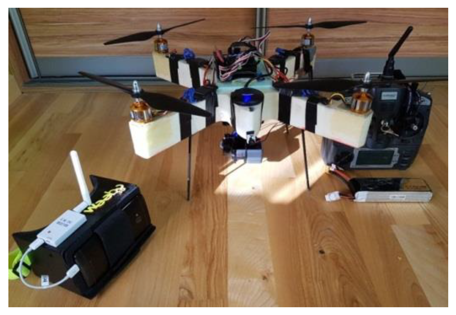
The approach proposed in this paper is the use of images acquired from low altitudes using an action camera, and dense image matching algorithms to high accuracy determination of the volume of excavations. The presented approach has a practical application in geodetic industrial measurements. As part of the research work, an unmanned aerial vehicle was designed and equipped with a GoPro with a wide-angle lens.
The contents of the paper are organised as follows.
Section 1 gives an introduction and a review of related works. In
Section 2, methodology and a low-cost UAV system with an action camera are presented. In
Section 3, research and data acquisition are presented. In
Section 4, photogrammetric data processing is presented.
Section 5 contains the results of tests from individual stages of image processing.
Section 6 discusses the results in the context of experiments carried out by other researchers.
Section 7 contains conclusions from the investigation and describes further research.
3. Research
3.1. Study Site and Data Set
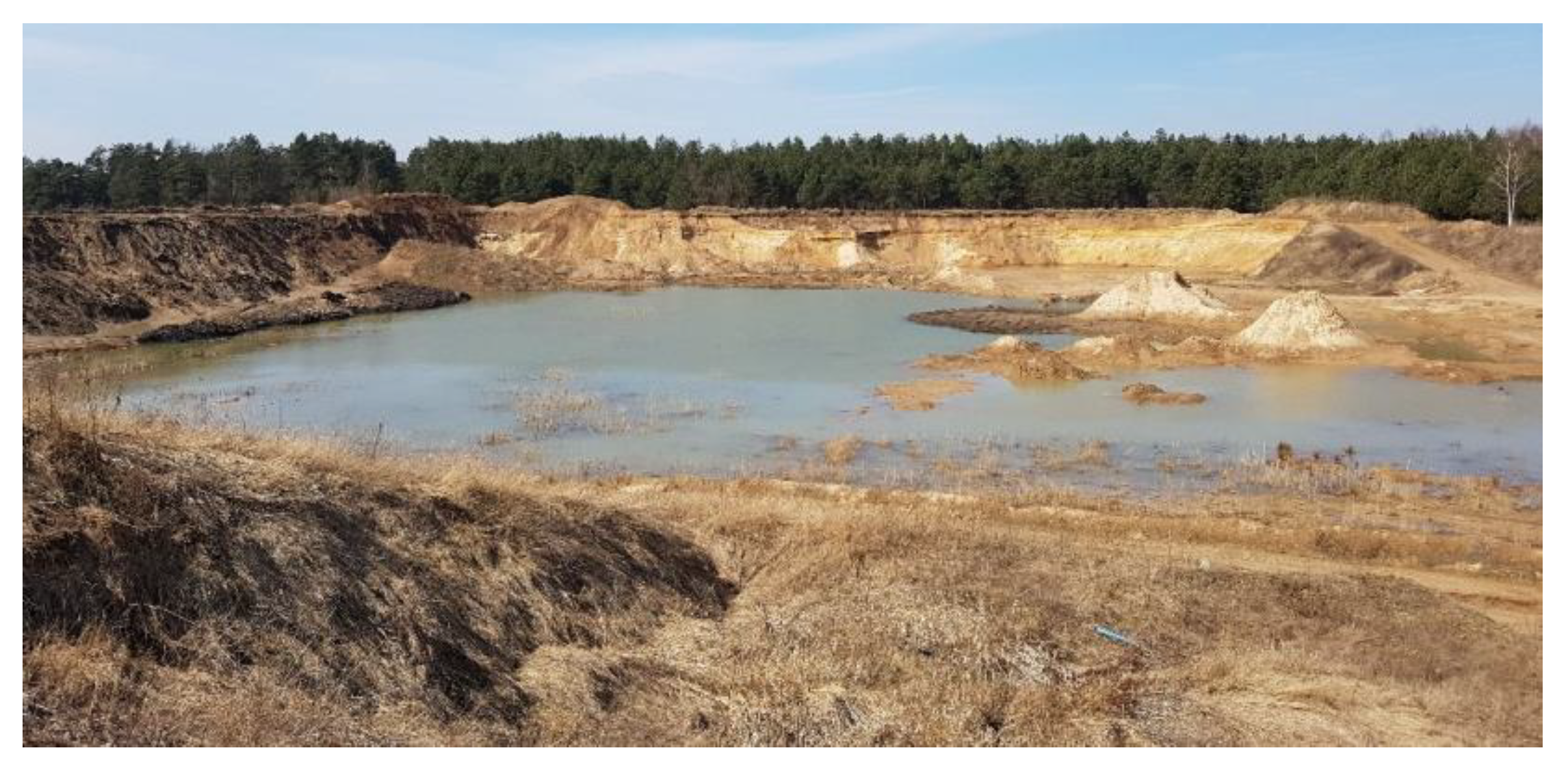
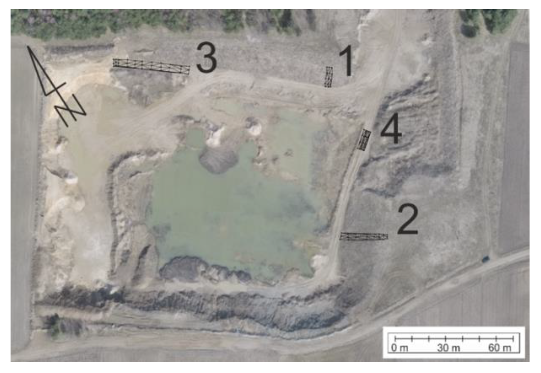
The selected object for DTM accuracy tests is the inactive opencast gravel mine, located in the Podlasie voivodship in the village of Mince (Poland) (
Figure 5 marked with a red rectangle). The area south of the mine is completely exposed, there are no trees or bushes. About 50 m to the east and west of the mine is a high, mixed forest. The biggest problem for photogrammetric flight, is the northern part of the object, due to its proximity to the forest wall—approximately 20 m from the mine.
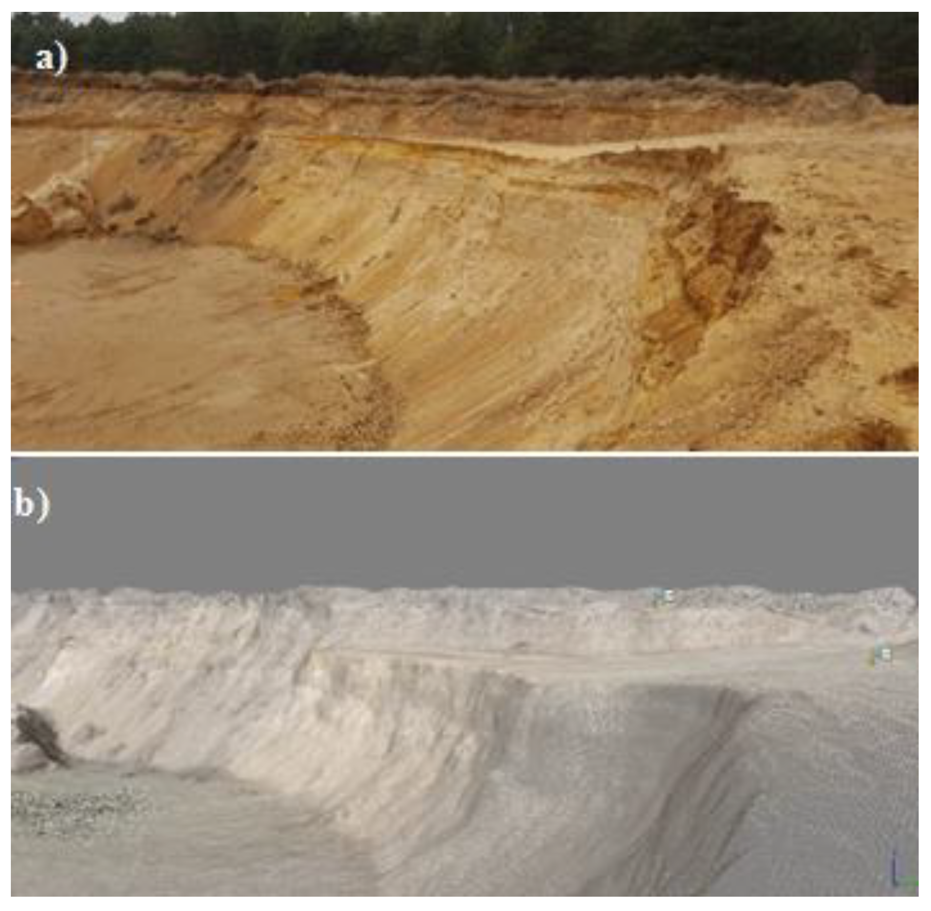
The mine itself is entirely free from high vegetation. On its surface, clay and yellow sands prevail and only some of the slopes are overgrown with thickets. The middle part of the mine, the lowest part, is flooded with shallow water (
Figure 6). This object was selected due to the rather close location to the place of residence of the author of this work and due to the high denivelations of the area, up to 12 m between the highest and the lowest point of the excavation. In this area there are also slopes with different degrees of inclination and different land cover types—both grassy and sand areas can be distinguished.
The entire mine occupies about 6 hectares, and its shape is similar to a rectangle. The photo in
Figure 6 was taken from the eastern part, showing the western part of the excavation.
3.2. Measurements of Photogrammetric Network
A fundamental issue in flight planning to obtain images from low altitudes is the design and in situ measurement of a photogrammetric network. The photogrammetric network is a set of points with specific coordinates that can be uniquely identified both in the field and in the image. As is well known, the disposition of the GCPs is one of the most influential factors in the precision of photogrammetric surveys from UAV. Because a nonmetric camera was used, we decided to distribute the GCP evenly or homogeneously in the edges of the photogrammetric block but also in the centre of the area [
10,
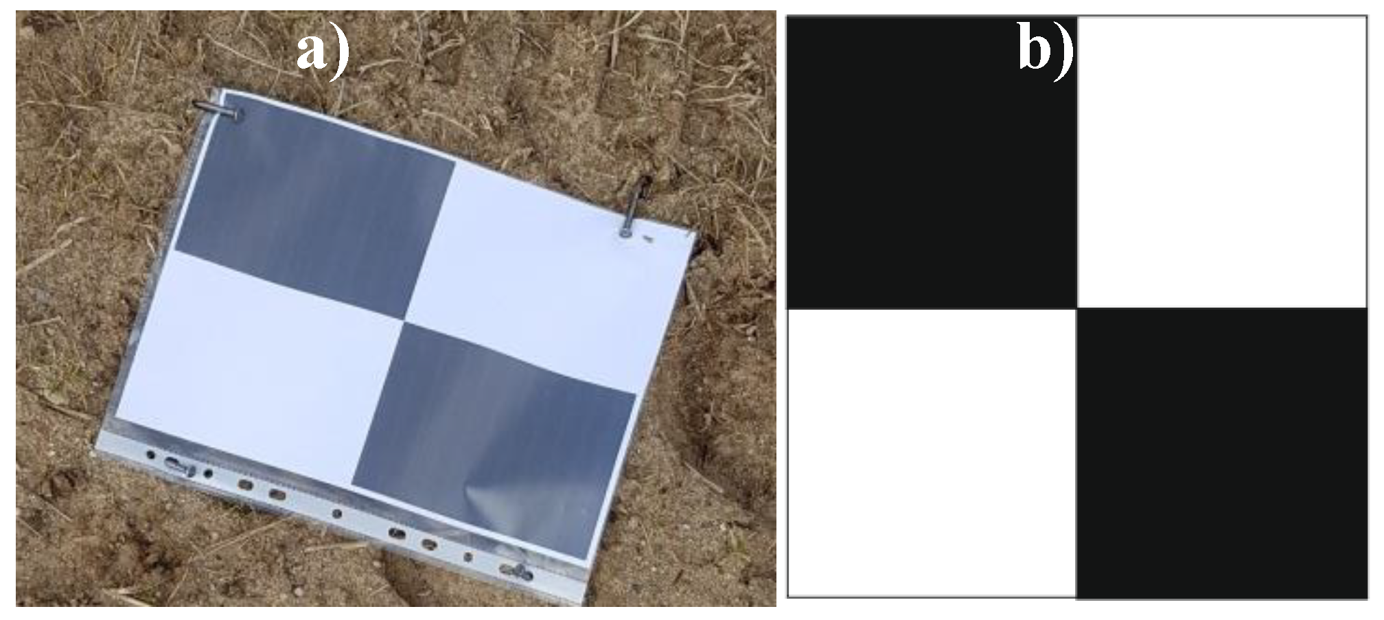
11]. In UAV photogrammetry, it is recommended to use signalised-Ground Control Points (GCPs). The use of signalised-(GCPs) in the form of a character with a white and black chessboard allows for the unequivocal identification of the point both in the image and in the field.
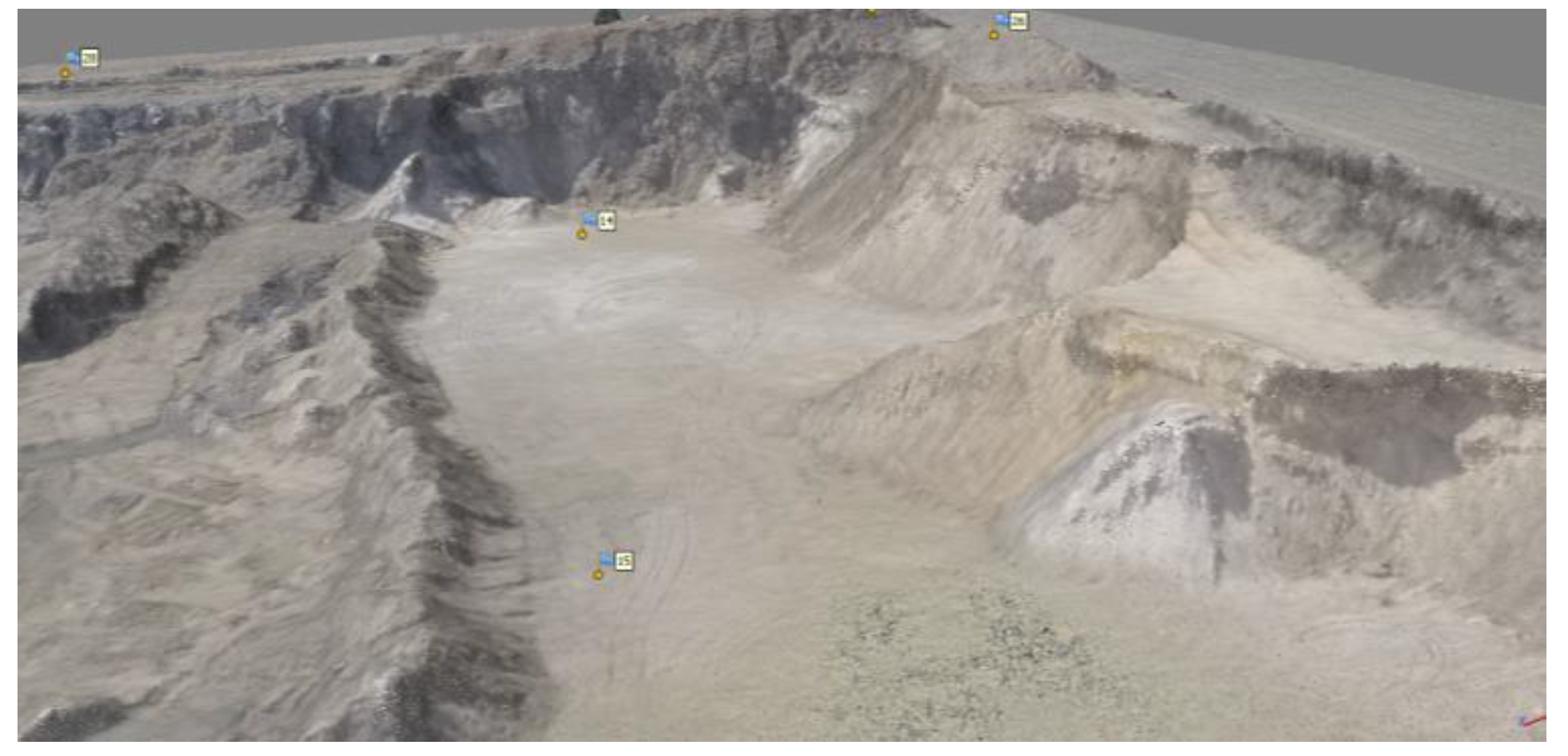
In this work, a photogrammetric network using GPS-RTK measurement techniques was established. Control points were marked with a special sign (
Figure 7), and 28 evenly distributed throughout the photogrammetric block control points were measured.
The measurement of the network points was carried out with the Trimble SPS882 receiver in PL-2000 zone 8 coordinate system (EPSG: 2179), and in the PL-KRON86-NH elevation system. The correctness of the height measurements was verified by measuring the classic geodetic points- class III (points 819312-11120 and 819312-11220) located within 3 km from the tested object. Deviations on points did not exceed 5 cm. The average value of the position dilution of precision (PDOP) coefficient from the entire measurement was in the range from 1.2 to 1.8, and the number of satellites was from 12 to 17, which is a very favourable result. The standard deviation of 1σ average (68% confidence level) for 2D coordinates did not exceed 20 mm (average 10 mm), and for the height did not exceed the value of 25 mm (average 15 mm).
In the figure above (
Figure 8), check points are marked in red, and the control points are in black.
3.3. Data Acquisition
The photogrammetric flight was planned in the Mission Planner software, which is adapted to the APM 2.6 flight controller. Next, the flight altitude of the above ground level (AGL) was determined as 70 m, the flight speed was 7 m/s, and the direction of the flight was set at 121°. The direction is equal to the azimuth value, which was chosen in order to reduce the number of rows as much as possible. This was done in order to increase the efficiency of the flight, and thus to minimise UAV flight time. The value of the longitudinal and transverse coverage was 80%. During the measurement campaign, 353 images in 10 strips were acquired. Each strip contained 35 images.
3.4. Reference Measurements of the Excavation
In order to carry out the accuracy analyses of the digital surface model of the excavation, it was decided to measure the cross-sections of four slopes located on the study site. The measured slope profiles differ from each other by the angle of inclination, length and type of land cover (two of them are sandy surfaces, and two further grassy ones). The measurement was made by the RTK method using the GNSS Trimble SPS882 receiver. In the first profile, 15 points were measured, in the second—24 points, in the third—33 points, and the fourth one—36 points (
Figure 9).
The first test area was on the slope with the highest degree of inclination. This scarp was covered with high (about 30 cm), dry thicket. Five cross-sections were measured, in which each cross-section contained 3 points evenly spaced. The total area of this test area is 103 m2.
The second test area was on a slope with a slightly lower degree of inclination. This slope was also overgrown with 5 cm high grass. Eight cross-sections of the escarpment were measured on the entire surface of this area, in which each cross-section contained three points. The area of the area was 444 m2.
Test area number 3 was located in the driveway for trucks with a sandy surface. It is the longest of all the tested areas, and its surface area is 1189 m2. Eleven cross-sections of this driveway were measured, each of which had three points.
The last test area used for the analysis was the area with the smallest inclination. The total area is 123 m2. Four cross-sections were measured, each containing nine points. The area was sandy.
Additionally, the entire excavation area was measured to compare field measurements with numerical measurements made on a dense point cloud developed on the basis of images obtained from low altitudes. For this purpose, the entirety of the excavation was measured using the GPS-RTK method with a total of 652 points.
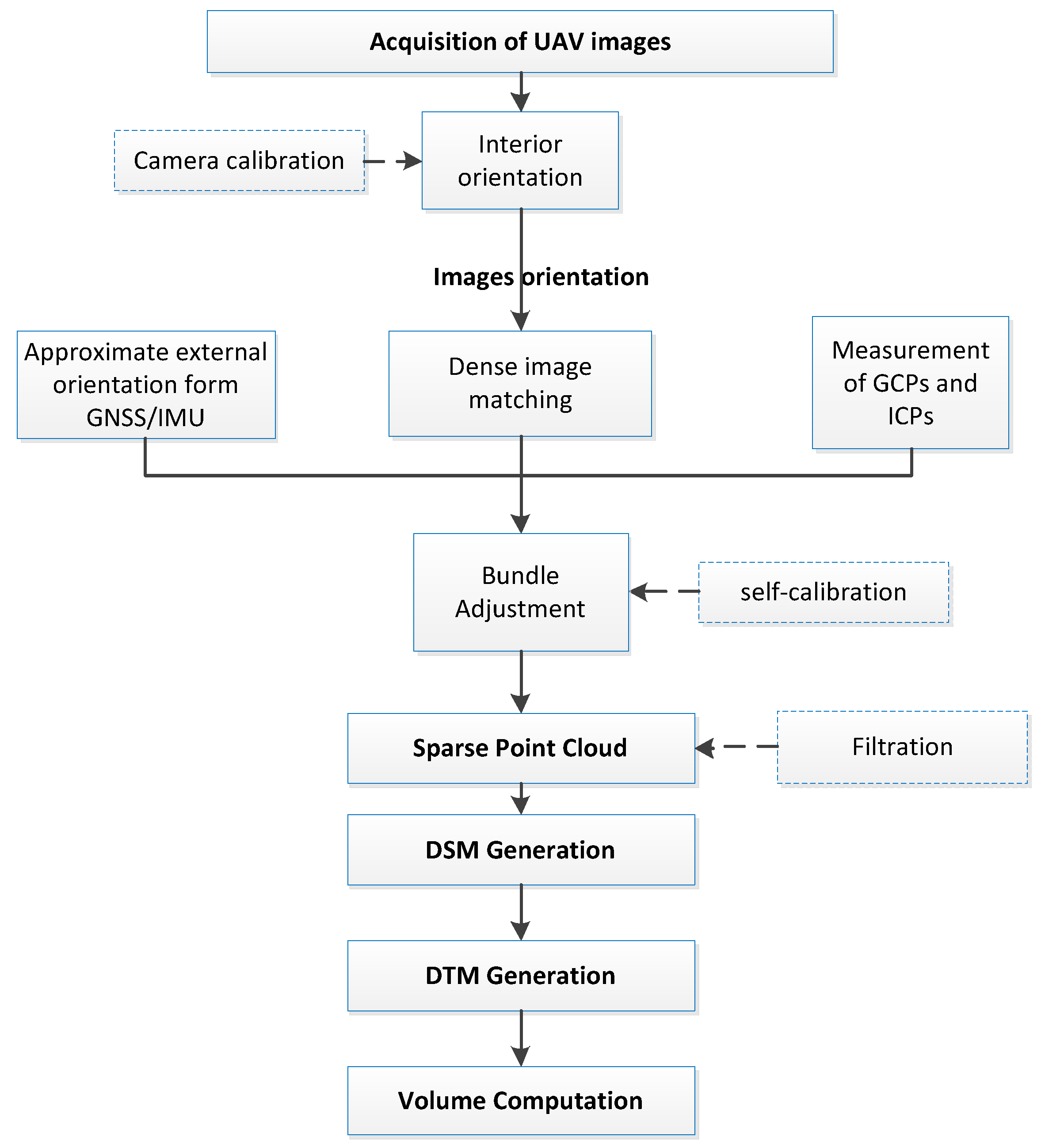
4. Photogrammetric Data Processing
Photogrammetric data processing is necessary to generate a geo-referenced 3D point cloud based on oriented images acquired from low altitudes. Based on the Structure from Motion (SfM) algorithms, a dense tie points network is generated to help determine the interior (self-calibration) and exterior orientations in the process of bundle adjustment. This process includes feature extraction and feature matching, estimation of relative camera poses from known point correspondences. The first processing step is feature extraction on every image in all subsets. In Photoscan the process is very similar to the well-known SIFT approach [
26], but uses different algorithms for a little bit higher alignment quality [
49]. These descriptors are used later to detect correspondences across the photos. In the next stage, a dense point cloud is generated, which is subjected to filtration to remove noise. In the next stage, a dense point cloud is generated, which is subjected to filtration to remove noise. For the filtration Photoscan has a tool to automatically classify the point cloud into “ground” and “non-ground” classes, which also uses Axelsson’s filtering algorithm [
50,
51]. The following parameters were set: maximum angle of 25 degrees not to exclude the points on excavation, maximum distance of 0.5 m and cell size of 5 m. On the basis of the prepared set of data, the Digital Surface Model (DSM) is generated, and the volume of the excavation is then calculated (
Figure 10).
The GNSS/INS system is installed in the multirotor model used in the study. Thanks to this, it is possible to determine the elements of the external orientation of the camera directly during the data acquisition. The approximate values of external orientation parameters (EOPs) allow the elimination of gross errors during the generation of tie points in coverage areas of images. Thanks to this, it is possible to accelerate the process images matching in the software, and also provide additional observations in the process of aerial-triangulation. The use of aerial-triangulation with additional observations (the approximate values of EOP) additionally strengthens the photogrammetric block and allows an increase in the accuracy of adjustment. The data from the navigation system mounted on the UAV board is characterised by low accuracy. Therefore, the strict determination of the position and orientation parameters (EOP) takes place only during the aerial-triangulation process after GCPs and tie points measurements.
4.1. Image Georeference
The APM 2.6 flight controller records all flight parameters in the LOG, which can be exported as TXT file after the UAV flight. In the file, there are, among others, the geographical ellipsoidal coordinates (B, L, H), where B is geographical latitude, L geographical longitude and H is ellipsoidal height in the WGS-84 flight system and three inclination angles ω, φ, κ. Because of this, it is possible to add georeference to images obtained from a UAV platform using the Mission Planner software. An important factor that allows the integration of flight parameters with photos is the appropriate synchronisation of the controller and camera clocks. The offset value between the time of the clocks is calculated so that the appropriate coordinates and angles of inclinations are adjusted to each photo. In addition, information that indicates the difference between the time the image was taken and the nearest, adjusted time of the recorded GPS position is displayed. In this study, the minimum value of this difference was 1 ms, and the maximum value was 216 ms (average 65 ms). These values result from the operating frequency of the GPS receiver. In practice, this means that with a flight speed of 7 m/s, the maximum position error caused by the difference of this time (for the size of 216 ms) is 1.5 m, because: 0.216 s * 7 m/s ≈ 1.5 m. Due to the low accuracy measurement of coordinates by the receiver (2.5 m), the offset between the location of the camera and the antenna of the GPS receiver (the difference in position is about 20 cm both horizontally and vertically) has not been corrected.
4.2. Bundle Adjustment of Images
The bundle adjustment of images obtained by a multirotor was carried out in the AgiSoft Photoscan [
49] software. First, the acquired images were read and then a previously prepared text file containing approximate external orientation parameters was imported. Then, these elements were transformed from the geographical coordinate system WGS-84 to Mapping frame PL2000, in which the photogrammetric network and slope cross-sections were measured. The precision of the position of the image was set at 2.5 m and 3 degrees in the angular orientation. The align photos accuracy was established as high. The maximum number of characteristic points in each image that was taken into account during the mutual orientation was 20,000. The limit of tie points for each photo was set to 5000. The result of this process is a dense cloud created by tie points.
Camera Calibration—A Mathematical Model
Camera calibration is intended to reproduce the geometry of rays entering the camera through the projection centre at the moment of exposure. The calibration parameters of the camera are:
calibrated focal length—ck;
the projection centres in relation to the pictures, determined by x0 and y0—image coordinates of the principal point;
lens distortion: radial (k1, k2, k3) and decentering (p1 and p2) lens distortion coefficients.
In the case of action cameras, there is one large FOV in wide-angle viewing mode. The calibration process plays a very important role in modelling the distortion of the lens. The model of internal orientation used in the research was applied in the Agisoft Lens based on the modified mathematical Brown Calibration model [
52].
In the case of large distortion, as in the wide-angle lens, radial distortion will be extended by additional distortion coefficients: 1 +
k4r2 +
k5r4 +
k6r6. Ideally, radial distance will have the form:
where:
When taking into account the influence of distortion, image coordinates will take the form of:
where:
k1, k2, k3—polynomial coefficients of radial distortion;
p1, p2—coefficients describe the impact of tangential distortion;
x″, y″—image coordinates of point repositioning based on the distortion parameters;
fx, fy—are the focal lengths expressed in pixel units;
cx, cy—are the principal point offset in pixel units;
u, v—are the coordinates of the projection point in pixels.
In the process of the bundle adjustment of image block, the Interior Orientation Parameters of the camera were computed, i.e.,
f,
x0,
y0,
k1,
k2,
k3,
p1,
p2. As we know, the process of laboratory calibration method is carried out indoors, free from the influences of weather and other environmental factors and specialised equipment. The values were compared because we want to check the correctness and accuracy of the internal orientation parameters (IOPs) of Camera. The values of these elements are presented in
Table 3 and compared with the camera calibration results carried out in laboratory conditions based on a photographed chessboard.
It was assumed that the values of the elements of internal orientation from the self-calibration process were more accurate because a large number of photos and field points of the photogrammetric network were used, as well as a large number of tie points in the pictures. The results from the self-calibration process were used for further experiments. Furthermore, for this reason, previously estimated Internal Orientation (IO) parameters have been used as approximated values.
In the next step, relative and external orientation was made by generating a dense network of tie points, and then coordinates of Ground Control Points were imported and edited.
After generating a sparse point cloud, the task of which was to merge images into one block with tie points, it was necessary to do bundle adjustment. In the bundle adjustment procedure the projection of a 3D scene point X ϵ R
4 to a 2D point x ϵ R
3 is modelled as the perspective projection:
The calibration matrix K describes the internal orientation of camera, while R and t are models of the rotation and translation necessary for transformation from the world coordinate system to the camera coordinate system. The main task of the bundle adjustment process is to optimise all
m cameras (
, I = 1, …,
m) as well as all points (
= 1, …,
n) simultaneously, starting from an initial estimation. This step is modelled as a least-squares minimisation of a cost function with nonlinearities in the parametrisation (the parameter vector θ contains structure and camera estimates, while
(θ) describes the corresponding projection of 3D points in the image of each camera):
Based on this dependency, the reprojection error is modelled as the squared Euclidean distance d between image point and projected point (in Euclidean coordinates).
For this purpose, the coordinates of the control points were imported and then identified and measured on each photo. The error value σ0 after block alignment was 2.25 pixels–3.44 μm. The total number of control points used during the alignment process was 21. Independent Check Points had been attempted to distribute most evenly across the block of images, and their total number was 7 [
53,
54].
The accuracy errors obtained on the control points are about 0.019 m to 0.022 m. On the other hand, the accuracy at the check points has slightly higher values and ranges from 0.025 m for the Y coordinate to 0.034 m for the height coordinate. Error values at check points are counted as the differences of the respective coordinates of points measured in the field with the coordinates determined during the block adjustment. The total error in the identification of the control points in the image was 1.1 pixel, and the check points 1.0 pixel.
The camera position error values measured by the inaccurate GPS mounted on the UAV reach values from 2.91 m for the Y coordinate to 5.32 m for the Z (height) coordinate. As mentioned earlier, the position data provided by the onboard GPS receiver were not very accurate and does not affect the accuracy compensate block of pictures or reduce the number of control points needed. These data significantly accelerate the initial process of matching images and also the process of coordinates measurement of control points in the images.
During the flight the camera was mounted on a gimbal the task of which was to keep it in the theoretical horizontal plane (the theoretical value of Pitch and Roll angles should be 0). The measurement accuracy of the gyro placed in the gimbal is 2–3 (°). The values of platform orientation errors in the pitch and roll directions are 2.81 and 0.84 degrees respectively, which means that they are within the range of measurement error of angles by the gyroscope used. During the flight, there were gusts of wind through which the UAV was subjected to twists, which resulted in the platform’s orientation error in each of the three directions, especially in the yaw direction at the level of 7.73 degrees.
4.3. Generation of 3D Point Clouds and DSM
The generated digital surface model of the open cast mine based on dense point cloud (initially, a sparse cloud was generated). Before generating a dense point cloud, a Bounding Box was selected to define the boundaries of the study area. This range was marked to include the mine, but to exclude the forest. This allowed the acceleration of the process of building a dense point cloud. In order to obtain high-quality data, the following parameters were adopted to generate the point cloud: Quality—High (size of the source images was downscaled to 50%), Depth filtering—Aggressive (this filter mode removes vegetation and softens the surface).
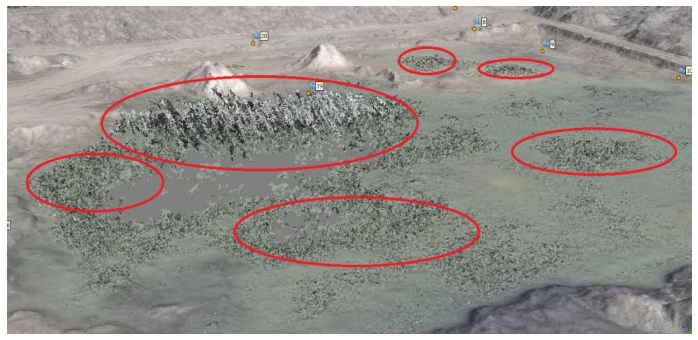
When generating a dense point cloud in the areas where water was located, large errors occurred in the location of individual points (
Figure 11). Theoretically, a flat surface should be created, but because the water in some of the photographs has been photographed in white (reflected sun from its surface), and in other pictures in green, the software wrongly selected the homological points in individual photos. Another reason is the incorrect generation of homological points in areas with the same texture, e.g., where there was only sand in the image (homogeneous areas). This resulted in errors in the component altitude of the points, reaching even 6–7 m. It was decided to completely remove these points from the point cloud during filtration because they were generated incorrectly.
In this way, a prepared point cloud was used to perform accuracy analyses (
Figure 12).
The value of the reprojection error was 2.25 pixels. The value of this error is characterised by the accuracy of positioning points in the cloud. The number of points created is 20.58 million. The average density of point clouds is 229 points/m2, and its resolution is 0.066 m/pixel.
5. Results
This section presents the results of the accuracy analysis of dense point clouds and digital elevation models of excavation. The analyses focused on examining the correctness of terrain representation by the obtained point cloud. Moreover, the accuracy of the point cloud based on its density was examined. The volume of the entire excavation obtained from dense image matching and the volume calculated on the basis of GPS-RTK measurements was also compared.
The numerical model of the mine generated on the basis of the point cloud visually reproduced very well. DTM was obtained by the filtering process of point clouds by using geometrical values like distances and angles as filter criteria (based on Axelsson’s approach) [
50].
In the foreground in the figure below, lines of discontinuity can be seen (transition from a horizontal plane to a plane that is almost vertical), which reproduced quite correctly (
Figure 13).
5.1. Comparison of the Volume
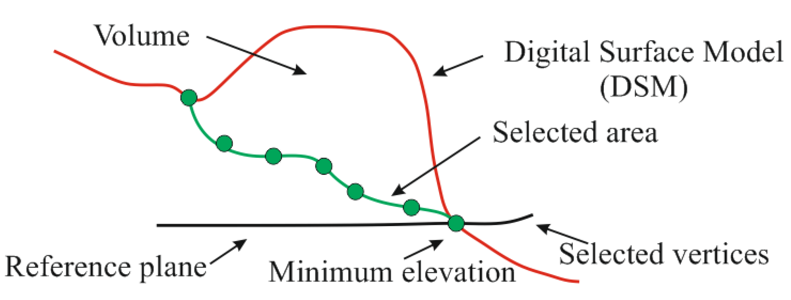
The volume of the excavation was calculated using two methods. The first way consisted of determining the volume based on a dense point cloud. The second one consisted of calculating the volume on the basis of previously measured characteristic points of the mine using the GPS-RTK method. The volume’s Equation (7) for each point will be:
where:
Vi—partial volume at the point,
GSD—Ground Sampling Distance (m)
Zij, TER—is the elevation of the pixel of the flat terrain (reference)
Zij, UAV—is the elevation of pixel ij of the model based on photogrammetric procedure (SFM) using UAV images.
The above figure (
Figure 14) shows the method of determining the volume above the reference plane assumed in the experiment. The volume is determined above the reference plane, which is the minimum elevation of the area of interest.
The results obtained were compared with each other. The calculated volume from the point cloud was 5,032,619 m
3 whereas the volume calculated on the basis of 652 points measured by the GPS-RTK technique in the mine was 5,028,656 m
3.
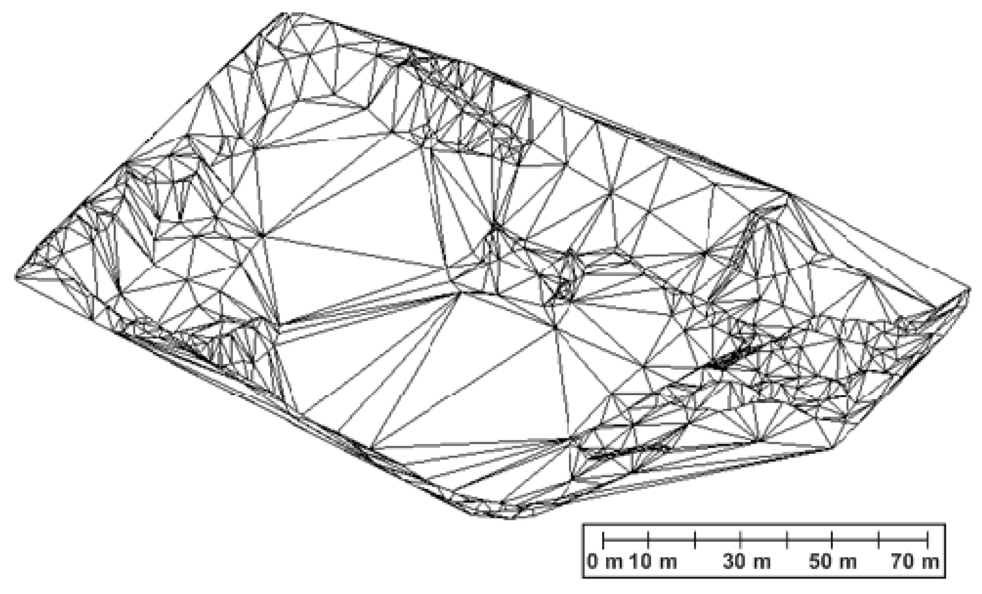
Figure 15 shows the reference Triangular Irregular Network-Digital Terrain Model (TIN-DTM) model in generated on the basis of the GPS-RTK technique.
The difference between the calculated volumes from two different methods is 3963 m3, which is just under one percent of the difference in volume between them. Based on these results, it can be concluded that the volumes obtained do not differ significantly (volume difference below 1%), which means that the volume measurement by a photogrammetric method using low-cost UAV finds its application to this type of measurements.
5.2. Analysis of the Accuracy of Digital Eleveation Models (DEMs) by a Dense Point Cloud
Four test areas were used for this analysis, the size and distribution of which is shown in
Figure 10. In the Global Mapper software [
56], the points measured using the GPS-RTK technique of individual test areas were imported, and then the TIN model of these points was generated resulting in a vector model. In this way, the created model was used as a reference model to which the point cloud was compared. DEMs of difference (DoD) highlighting the differences between the UAV model and the reference measurement were created. Differences in models were determined based on Equation (8):
where:
Zij, GEO is the elevation of pixel ij of the reference model measured by classical geodetic techniques;
Zij, UAV is the elevation of pixel ij of the model based on photogrammetric procedure (SFM) using UAV images.
On the basis of parts of the point cloud and the created reference models, proper analyses were carried out. In order to make a good visualisation, the red points represent points located above the reference model and the blue points are located below the reference model. For each test area, an appropriate visualisation was performed in the CloudCompare software [
57], to show the distribution of differences in the height of the point cloud in relation to the reference model. Additionally, a graph of deviations was created.
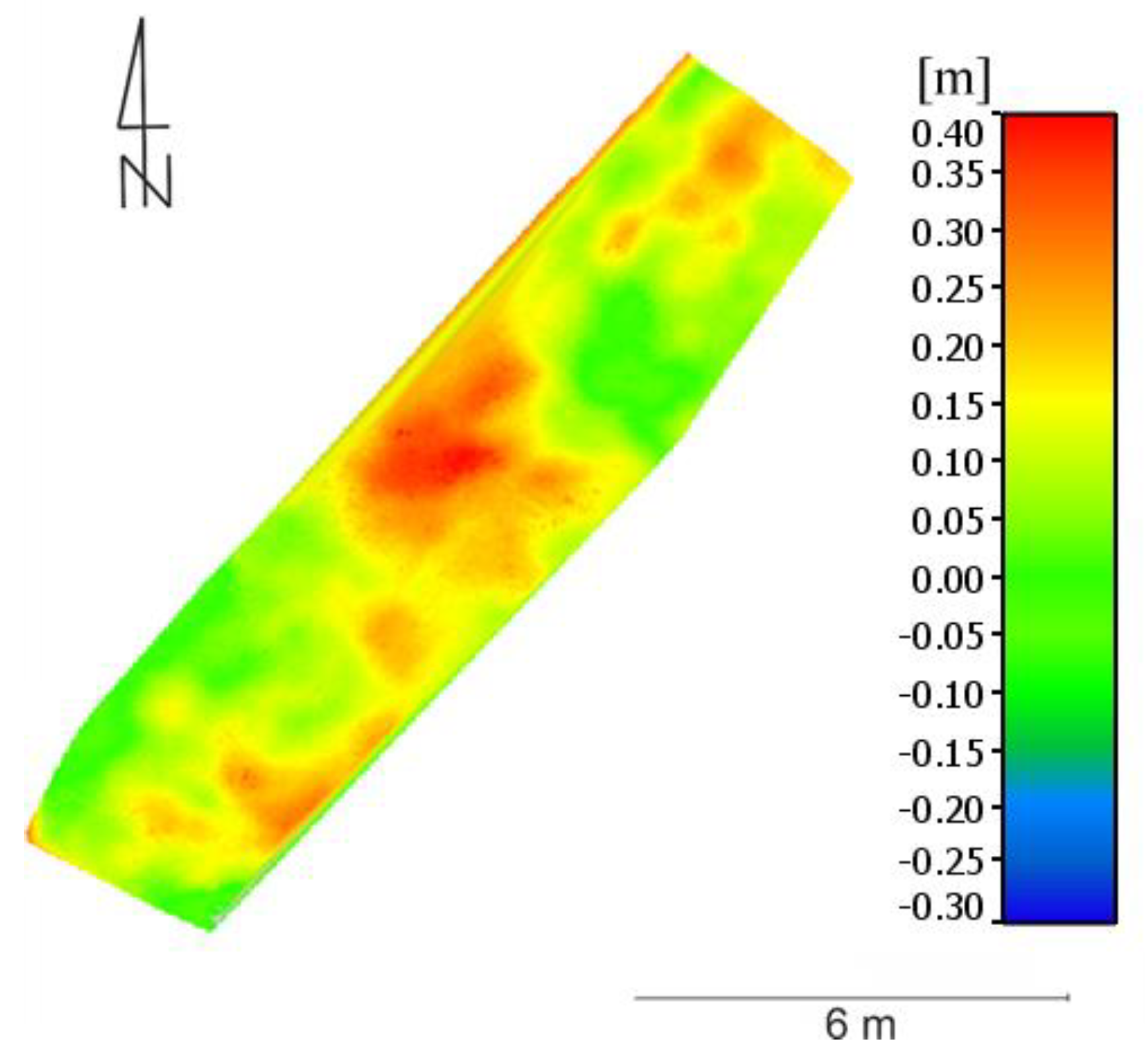
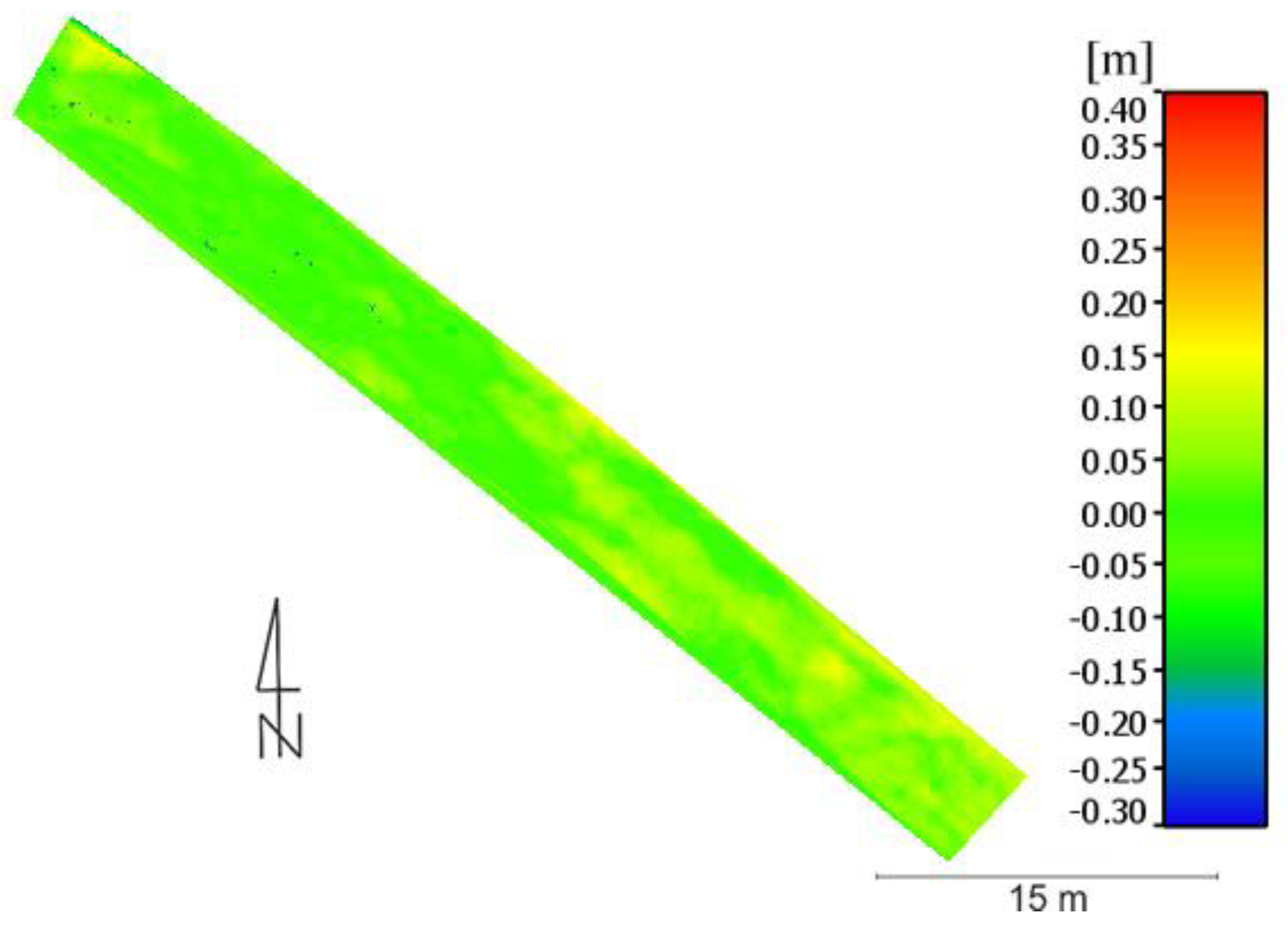
For Area 1, the distribution of deviations is shown in
Figure 16. Based on the following graphics, it can be stated that they best represent the measured model, the points of the cloud located in the north-east, and the south in the central part of the test area. The maximum values of height deviation reach 0.40 m and they concern the central part of the studied area. Such large deviations in this place are most likely caused by the fact that the highest thickets were in this place, which makes the point cloud altitude higher than the reference model measured in situ. Thickets have been found throughout this test area, which results in the fact that most of the cloud points are located above the reference model.
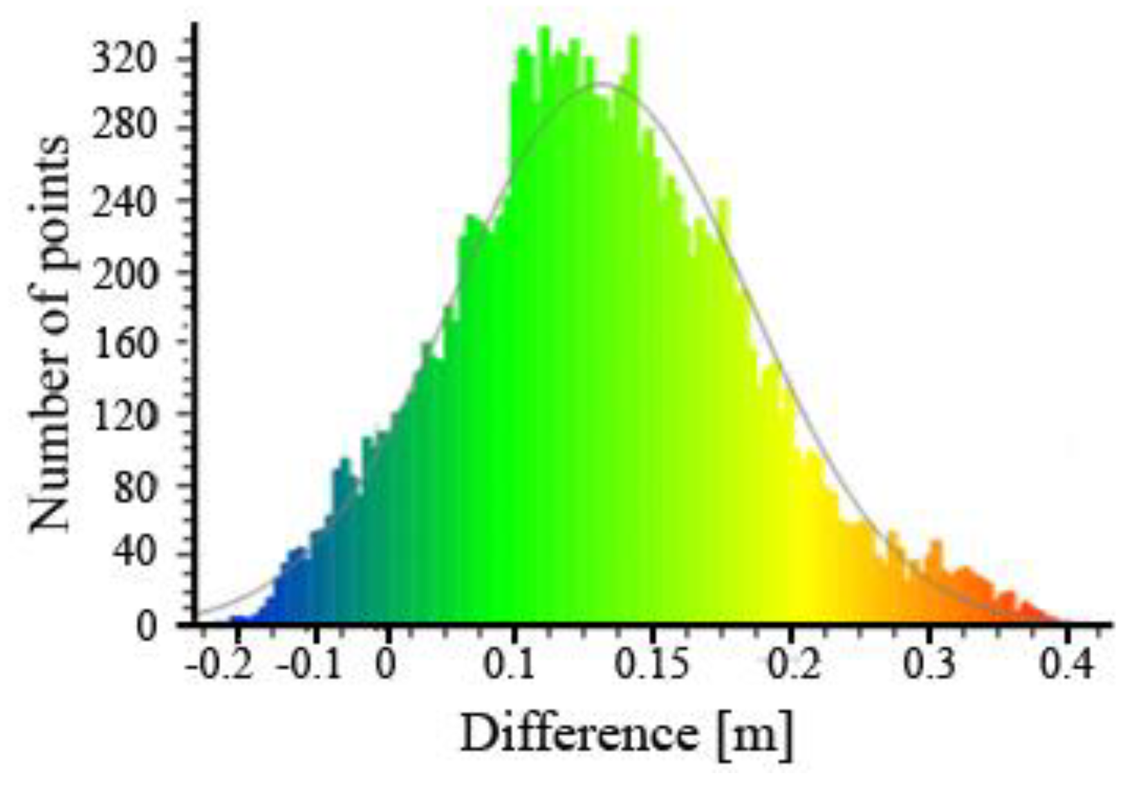
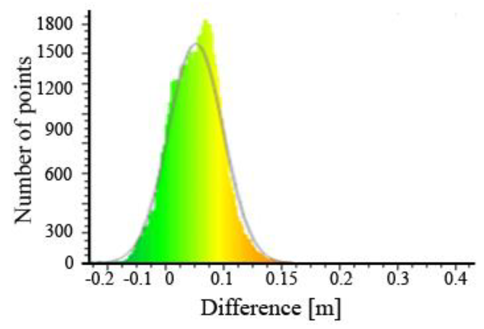
The number of points from which the cloud of the first test area was built is 15,184. Subsequently, the deviations obtained were analysed statistically and presented using a Gauss model (
Figure 17).
The average deviation value was 0.13 m, and the standard deviation of 0.09 m.
Figure 17 shows that most of the cloud points (as many as 3732) are in the range from 0.10 to 0.15 m above the reference area. It can also be seen that the number of cloud points located below the reference models is relatively small and amounts to only 955. The type of ground covering means that more points from the point cloud are found above the reference model. In this case, it is high thickets, which inflates the values of the height of the cloud points in relation to the reference model, despite the use of point cloud filtration to obtain DTM.
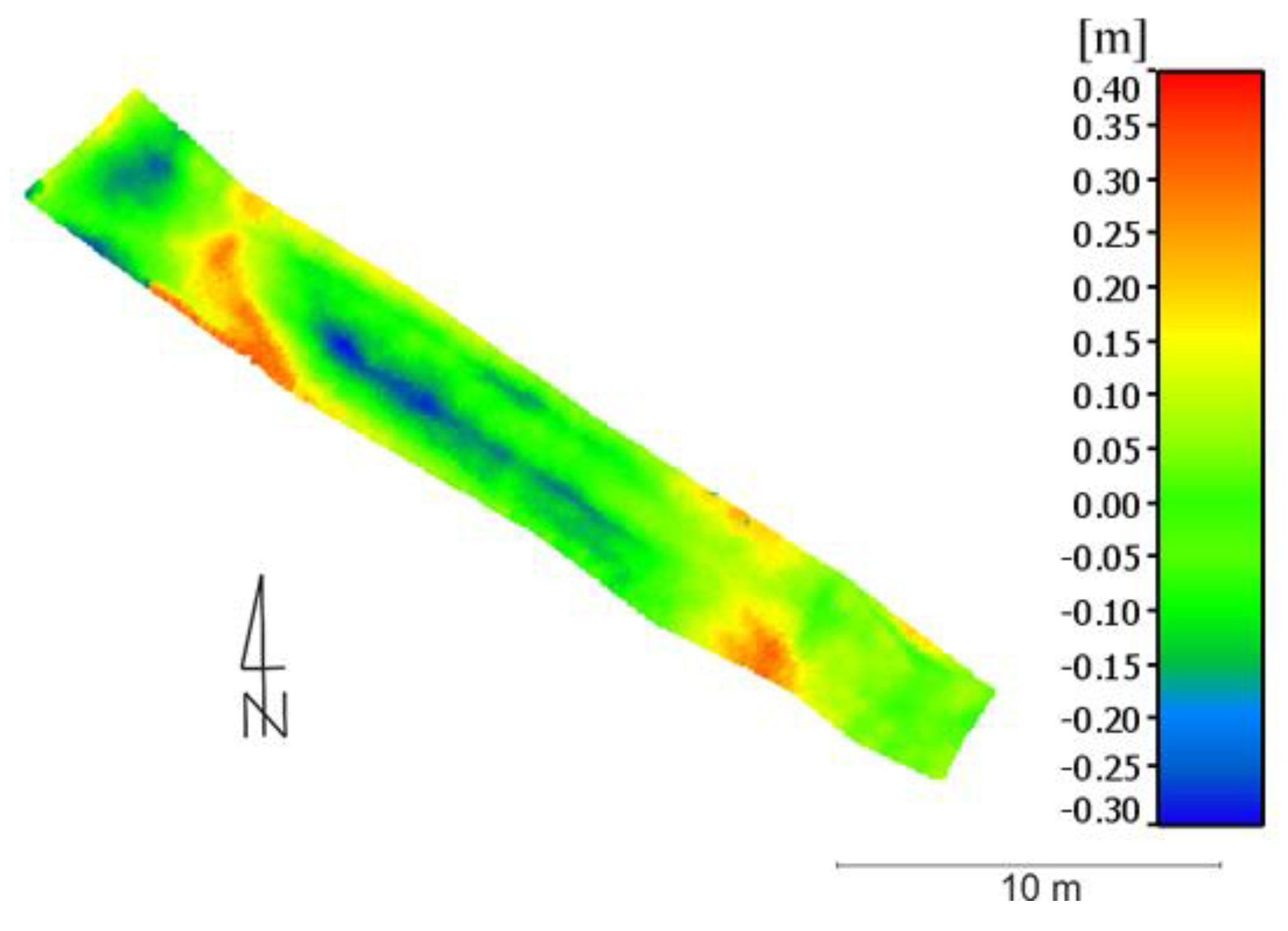
In the second test area (
Figure 18), as in the previous one, there were also thickets, but much lower, because its maximum height was about 0.05 m. The entire test area was located on a slope with a reasonably large inclination. The values of the height difference between the point cloud and the reference model are in the range from −0.25 to 0.24 m. The most significant negative differences (cloud of points located below the reference model) are located in the central part of the studied area. The author of the work believes that this is the result of a small terrain gap caused by the tyres of off-road motorcycles, and the direct measurement of GNSS on this section was relatively rare which caused excessive generalisation of this area, whereas the most significant positive differences occurred in the south-eastern and south-western part of the studied area.
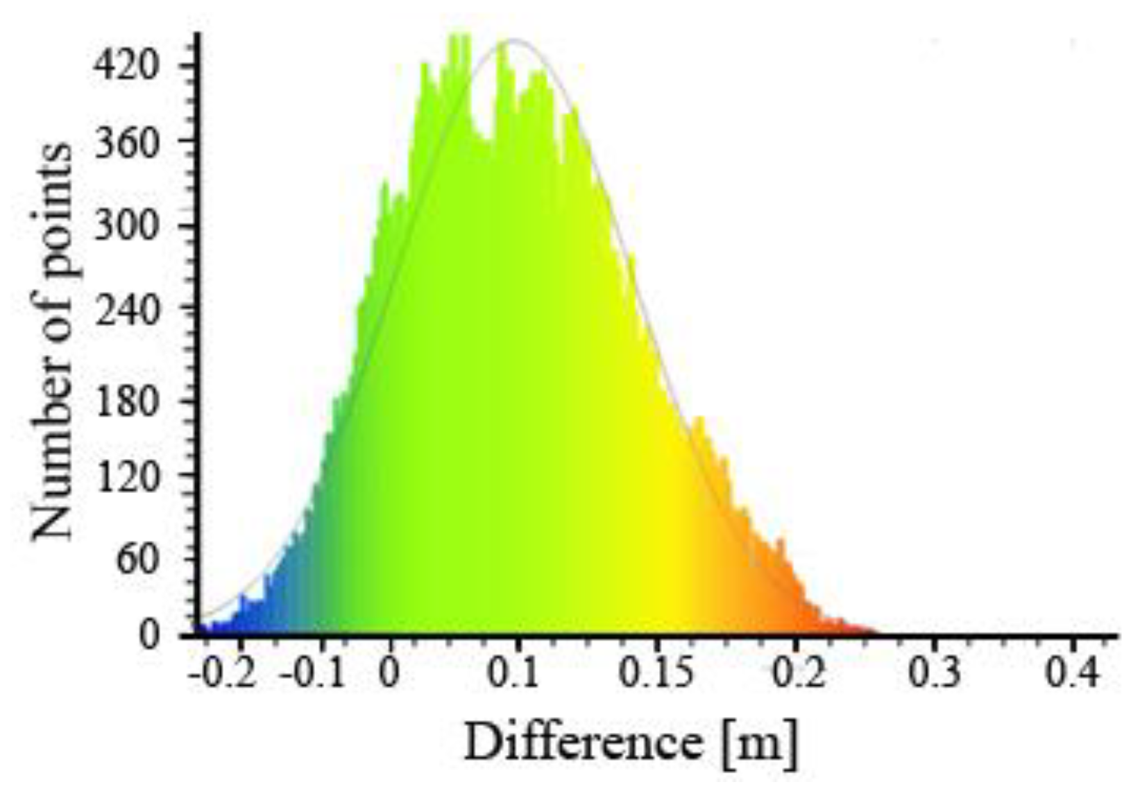
The total number of cloud points in this test area was 31,696. After using a Gauss model, an average deviation value of −0.02 m was obtained, while the standard deviation was 0.08 m (
Figure 19).
Most points of the cloud in the case of Test Area No. 2 are in the range from −0.05 to 0 m.
Figure 19 also shows that there are more clouds points below the reference model than the above.
The Third Test Area (
Figure 20) was located on a sandy, sloping surface that was once used as an exit route from the mine for trucks and excavators. This area was quite flat, fairly uniform, with a sloping surface. In this test area the smallest test height deviations were obtained, which range from −0.10 to 0.10 m. The most significant are the positive deviations, which are mostly in the south-eastern part of the area. In the north-east part, the areas with the smallest deviations are dominant.
The Test Area No. 3 cloud had 55,925 points. The mean value of the height deviation was 0.03 m with a standard deviation of 0.04 m (
Figure 21).
Figure 21 shows that most of the points of the cloud are in the range from 0 to 0.05 m. This means that in this test area a point cloud was obtained, mostly located above the created reference model.
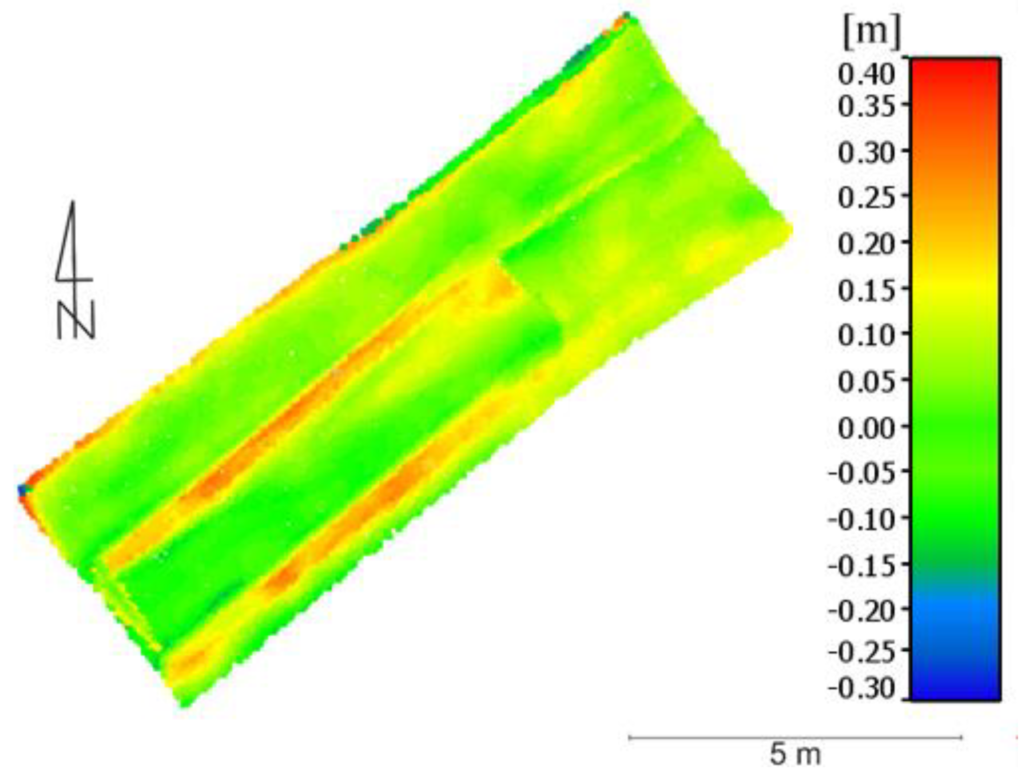
The last (fourth) test area (
Figure 22) is the lowest of all the previous ones. It presents a fragment of a sandy road. This area is also characterised by a very small slope (the smallest of all test areas). In the reference model created on the basis of the previous measurement of direct GNSS, ruts formed by trucks were taken into account, which means that additional points were measured in places where ruts were found. The highest height deviations between the point cloud and the reference model occur in places where the rut described above was located. In the graphic (
Figure 22), it is clearly visible in orange, where the deviation value reaches 0.20 m. The points of the cloud do not clearly reflect these ruts, which are located higher than the reference model. In the remaining area of the studied area, altitude deviations are already lower and range from −0.05 m to 0.05 m.
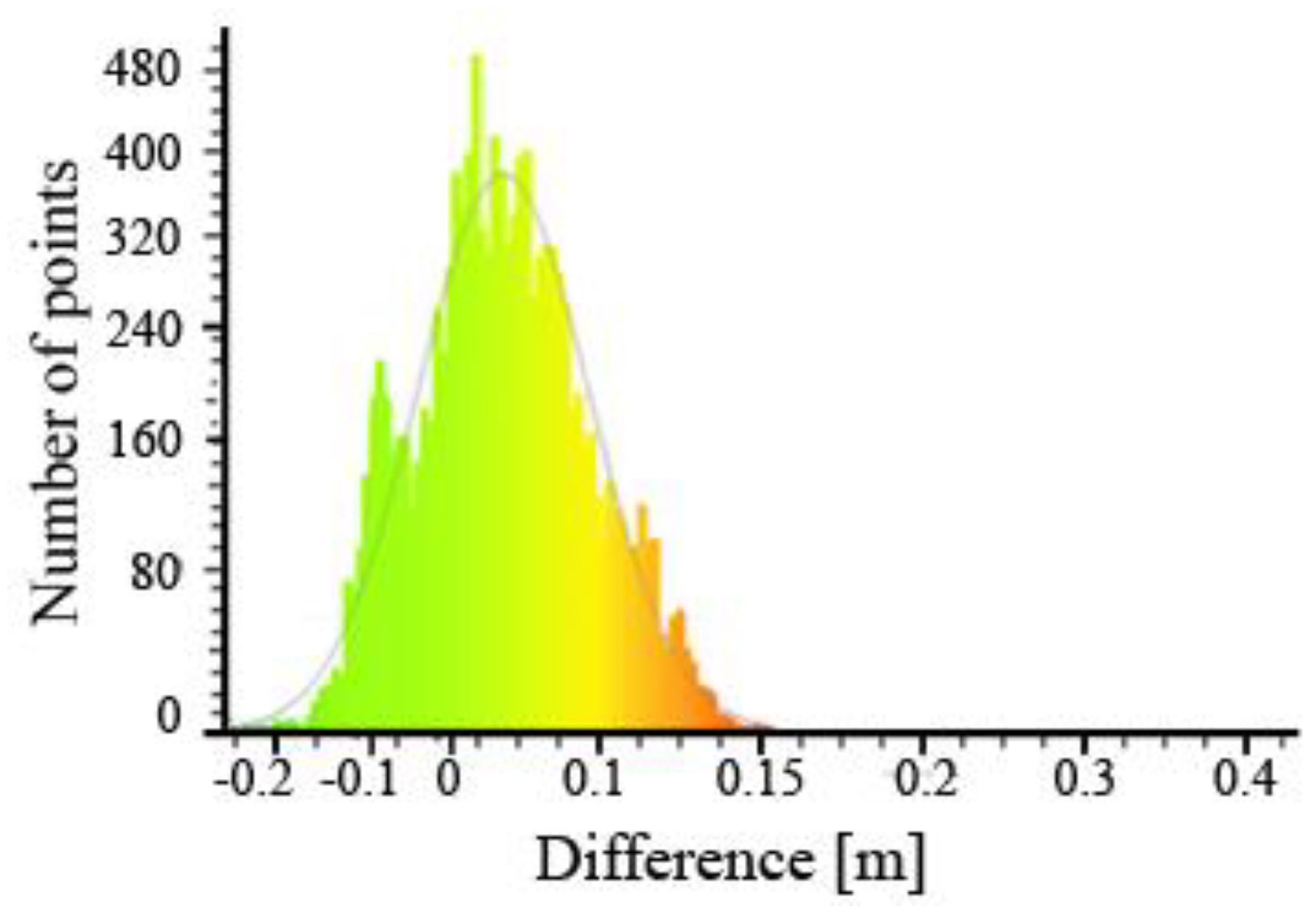
The total number of points in the cloud of the Test Area No. 4 was 13,325. After using the Gauss model, the mean value of the altitude deviation is 0.01 m with a standard deviation of 0.06 m (
Figure 23).
The results presented in
Figure 23 confirm the fact that the cloud points were mapped above the reference model in rutted areas. This is evidenced by the overwhelming number of points above the reference model.
5.3. Density and Completeness of the Point Cloud
A dense point cloud is the result of the application of special algorithms for matching images in a balanced block of images. Due to the fact that the UAV performs a relatively low flight over the terrain, a high resolution of images is obtained, which significantly affects the density of the point cloud reached.
The quality of the digital model of the excavation depends on the completeness of the point cloud and its density. One of the important parameters for assessing the quality of obtained DTM is the density of point clouds. This parameter depends on: the ability to highlight details directly related to the site and the quality of identification of characteristic points. Most often the density of point clouds is determined by the number of points per unit of area. The accuracy of the point cloud as a form of representation of the object as a whole is closely related directly to its density.
Due to the fact that a dense cloud of points is obtained using the dense image matching technique, their quality depends on the algorithms used and UAV image quality. Very often, during the generation of homological points, photogrammetric algorithms suffer from problems due to either the image quality (homogeneous areas, noise, low radiometric shadows). The aforementioned factors may cause noisy point clouds or difficulties in the extraction. Therefore, in order to more accurately assess the obtained DTM, we have also examined the density of the obtained point clouds and its completeness considering geometric and topological fidelity, amid the amount of missing data.
In the case of Digital Elevation Model creation, interpolation (based on Delaunay triangulation) is performed using the points around it. The relation is important: the higher the density of point clouds with low noise, the greater accuracy of interpolated altitude.
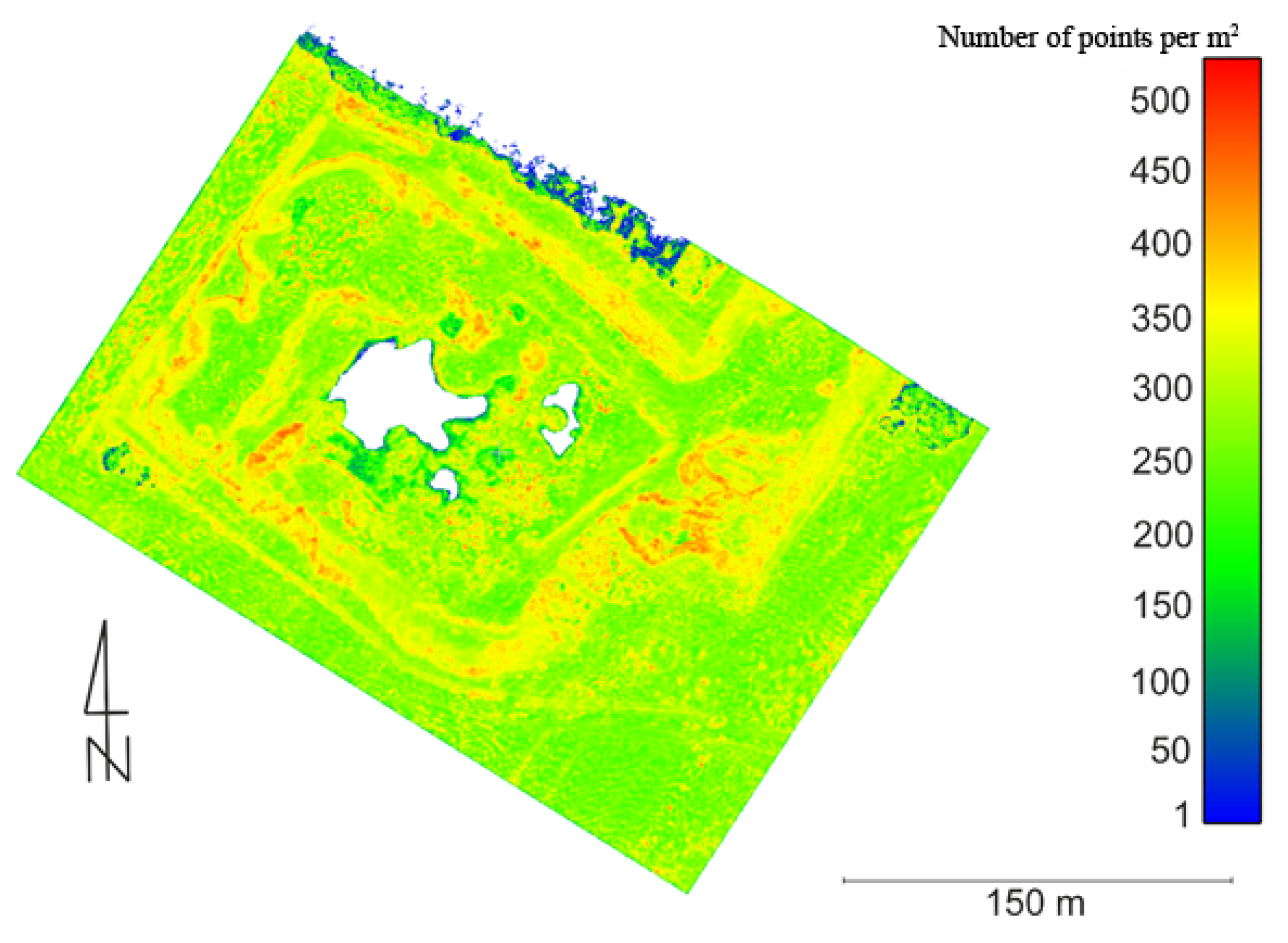
Figure 24 shows the distribution of the density of the point cloud, defined as the number of points per 1 m
2.
A density of about 200 to 250 points per square metre prevails in the area of the entire mine. There are no points at all in the middle of the mine, because there was water on which the height of the points was interpolated. Therefore, these points were removed during the point cloud filtration process. The smallest number of points generated is found on the crowns of trees in the northern areas and near places where there was water. A more significant number of points (about 350–450 per m2) occurs at the tops of individual embankments and slopes.
6. Discussion
In the presented study, a method of acquiring images from low altitudes using light and an efficient UAV platform was shown for the needs of developing digital 3D models of excavations and testing their volume.
On the basis of the analysis of test results in individual test areas, the average value of the height deviation ranging from 0.01 to 0.13 m was obtained (the highest deviation was obtained in Test Area No. 1, and the smallest in Test Area No. 4). Obtaining the highest value of this deviation in Test Area No. 1 indicates that the accuracy of the DTM created on the basis of UAV images has the effectiveness of the filtration applied for the area covered with thickets to extract the correct DTM. As part of the experiment, the accuracy of the digital surface model was examined by performing appropriate analyses on the point cloud. In the case of thickets occurring in the test object, it is difficult to conduct an appropriate filtration of the point cloud, which results in obtaining higher values of the height component in the obtained point cloud.
An analysis of the accuracy of the digital surface model obtained from UAV images was carried out and also described in Fras et al. [
58]. This article uses the quadcopter Microdrone md4-1000 and the Olympus PEN E-P2 camera. Next, the digital surface model was acquired and developed, obtained after the appropriate filtration of 11.17 million points of the point cloud. The accuracy analysis was carried out on the basis of check points measured with kinematic methods directly in the field. Eighteen check points were used whose heights were compared with the heights of the corresponding points on the point cloud. An average error value of 0.009 m was obtained on an altitude component with a standard deviation of 0.025 m. These values are lower than those obtained in the presented research. In the aforementioned work, the obtained photos have a resolution of 0.022 m/pixel, and they were acquired from 88 m (AGL height). Undoubtedly, the ground resolution of acquired images and altitude have a crucial role in the accuracy of the final results of the photogrammetry study.
In the case of the density distribution of the obtained point cloud, very similar results were obtained as in the article mentioned above. Lack of data in the point cloud is most often caused by insufficient coverage of photos or the presence of areas of homogeneous regions (e.g., sands). This causes problems in the correct operation of the automatic measurement of homologous points for the purpose of obtaining elevation data.
When analysing data on the accuracy of volume determination by UAV in the work of Raeva et al. [
59] and the work of Cryderman et al. [
60], and also the results obtained in the present experiment, it can be concluded that the use of UAV in this type of photogrammetric studies becomes an effective technology and less time-consuming in the case of volume measurement. Acquiring photographs of a given excavation are not as time-consuming as the physical measurement of points using the GNSS kinematic method. In this case, excavation photos in the village of Minka were obtained within 15 minutes, and the measurement of characteristic excavation points using traditional methods lasted almost the entire day (measured at 652 points with the GNSS kinematic method in about 8 hours). This is a huge difference in the length of time needed to obtain the appropriate measurements to calculate the volume. The results of these studies show that UAV images have the potential to provide adequate data for volume estimation with sufficient accuracy of around 1%.
7. Conclusions
The proposed method will allow the cheap and efficient monitoring of open pit mines and gravel pits. Thanks to the possibility of fast development of digital surface models of the excavation, it is possible to use them not only to calculate volume but also to track the construction process, monitor work progress and determine safety procedures (e.g., maximum slope level) during ongoing mining operations. The use of UAV technology allows the automatisation of the measurement process associated with the extraction, while reducing the error rates associated with the volume calculation. Using the appropriate method of filtering geospatial data, it is possible to achieve results that meet the accuracy criteria.
Analysing the accuracy of terrain mapping by a dense point cloud, the most accurate results were obtained in test areas where no vegetation was present. In the case of thicket in the test area, it is difficult to perform an appropriate filtration of the point cloud, whereby the heights obtained from digital measurements were characterised by a higher value than those obtained from direct measurements using the GNSS kinematic technique. Therefore, it can be concluded that the accuracy of terrain mapping by the point cloud is influenced by the type of surface of the studied area.
The use of UAV photogrammetry becomes an effective technology and less time-consuming when measuring volume. The acquisition of images by the UAV of a given excavation takes place much faster than the physical measurement of points by the GNSS kinematic method over its entire area. This is a big difference in the time needed to obtain the appropriate measurements to calculate the volume. The value of the obtained difference in the volume of the excavation of the study area obtained on the basis of data from the UAV, and the data from the physical measurement of points by the GNSS kinematic technique, differ by less than 1%. The use of unmanned systems does not require stopping work on the excavation and eliminates the need to enter a dangerous area, and also allows the measurement of inaccessible areas. The results of these studies show that the images obtained from UAV have the potential to provide adequate data to estimate the volume with sufficient accuracy. In the case of the photogrammetric method, irregular heaps do not pose a large technical problem, and the measured shapes are almost identical to those in reality, depending on the adopted photogrammetric assumptions.
The quality of the obtained digital surface model also depends on the completeness of the generated point cloud, because it affects the accuracy of the interpolated altitude. Lack of data in the point cloud is most often caused by insufficient coverage of photos or the result of filtration in which all protruding objects such as buildings or trees were removed in order to obtain a digital terrain model.
The results of the conducted research show that it is possible to build a low-cost UAV that will provide useful photogrammetric data. Based on the obtained results, it can be stated that the data obtained with a non-metric camera from the low-cost model of an unmanned aerial vehicle can be used to generate a three-dimensional point cloud using appropriate algorithms. Compared with the data obtained using traditional methods, satisfactory results were obtained, which indicate a high agreement between the compared models.
The quality of data provided by UAV does not differ from the data obtained by commercial unmanned ships of similar construction. The technical and measurement capabilities of the unmanned vehicle used in this work are therefore similar to commercial photogrammetric platforms of this category.
The performed tests are particularly important in the context of the use of images obtained from a low ceiling to accurately determine the volume of excavations. Future research will focus on the integration of two action cameras with mutual coverage in stereo mode, which will make it possible to increase the efficiency of imaging during one flight.


