Spatial Analysis Using Temporal Point Clouds in Advanced GIS: Methods for Ground Elevation Extraction in Slant Areas and Building Classifications

Abstract

Deriving 3D urban development patterns is necessary for urban planners to control the future directions of 3D urban growth considering the availability of infrastructure or being prepared for fundamental infrastructure. Urban metrics have been used so far for quantification of landscape and land-use change. However, these studies focus on the horizontal development of urban form. Therefore, questions remain about 3D growth patterns. Both 3D data and appropriate 3D metrics are fundamentally required for vertical development pattern extraction. Airborne light detection and ranging (Lidar) as an advanced remote-sensing technology provides 3D data required for such studies. Processing of airborne lidar to extract buildings’ heights above a footprint is a major task and current automatic algorithms fail to extract such information on vast urban areas especially in hilly sites. This research focuses on proposing new methods of extraction of ground points in hilly urban areas using autocorrelation-based algorithms. The ground points then would be used for digital elevation model generation and elimination of ground elevation from classified buildings points elevation. Technical novelties in our experimentation lie in choosing a different window direction and also contour lines for the slant area, and applying moving windows and iterating non-ground extraction. The results are validated through calculation of skewness and kurtosis values. The results show that changing the shape of windows and their direction to be narrow long squares parallel to the ground contour lines, respectively, improves the results of classification in slant areas. Four parameters, namely window size, window shape, window direction and cell size are empirically chosen in order to improve initial digital elevation model (DEM) creation, enhancement of the initial DEM, classification of non-ground points and final creation of a normalised digital surface model (NDSM). The results of these enhanced algorithms are robust for generating reliable DEMs and separation of ground and non-ground points in slant urban scenes as evidenced by the results of skewness and kurtosis. Offering the possibility of monitoring urban growth over time with higher accuracy and more reliable information, this work could contribute in drawing the future directions of 3D urban growth for a smarter urban growth in the Smart Cities paradigm.

1. Introduction

The smart city is an emerging concept referring to a technology-based solution for managing resources of a city [1]. Cities are known as complex and dynamic environments and their physical characteristics are changing over time. There is a desire to identify patterns of urban growth in three dimensions (3D), that is, growth both horizontally and vertically. Recent studies tend to collect accurate 3D geospatial data, process them using different methods, and visualise 3D cities, which are all still underdeveloped practices [2]. This paper focuses on two key deficiencies: (i) there is no reliable tool to extract ground points automatically in a large urban area including hills in a geographic information system (GIS) environment; (ii) there is no automated method for extracting building footprints in terms of the outer boundary of buildings in an advanced GIS environment. As GIS is often used for spatial analysis of urban big data [3], and is an important analytical tool in smart cities and urban planning [4], developing an automated method for extraction of buildings points from airborne light detection and ranging (Lidar) and their footprints in GIS would be beneficial to urban analytics. Otherwise, practitioners need to do all the required analysis in different tools encountering data exchanges issues including interoperability and missing information [5,6,7]. This paper aims to utilise airborne Lidar technology and advanced GIS tools to propose and evaluate new algorithms for ground points extraction from airborne Lidar data. Our proposed refined autocorrelation-based algorithm, building footprint extraction methods and visualisation are implemented and visualised in Environmental Systems Research Institute (ESRI) ArcGIS. These tasks are fundamental for applying 3D urban metrics for 3D spatial analytics and smart city data analytics, discussed in recent studies such as Li, et al. [8], Jing, et al. [9] and Rejeb Bouzgarrou, et al. [10].

American cities such as New York grew both horizontally and vertically in the late 1800s. In 1933, Le Corbusier advocated the concept of the ‘vertical city’ by proposing zoning of the cities and including tall buildings for living and working purposes [11,12]. Accelerated urbanisation and economic growth in the 1980s were two major drivers of vertical development of capital cities such as Tokyo [13]. The concept of a world city (e.g., New York, Tokyo and London with global socio-economic function) and the increased demand for space rather than land for new urban development is another driver for the vertical growth of the central business districts (CBDs) of cities [14,15,16,17]. Vertical development of urban areas formed through the construction of high-rise buildings results from policies, high demands for land development and land scarcity in urban areas [18].

Intensification policies to achieve compact cities [19], high-rise buildings in a high-density city form [20,21], and sustainable city strategies to achieve a compact urban form, have all created the trend for more compact cities. In addition, infill development often contains more development than its fringe areas and Brownfield development, a policy for redeveloping previously developed land [22]. This policy has been discussed as an effective policy to achieve sustainable compact cities in UK, Greece, Poland, Netherlands, France, Spain, Belgium and USA, [23,24], by minimising urban sprawl and putting less emphasis on greenfield development [22]. This type of development refers to constructing planned urban neighbourhoods with natural, landscape design on previously undeveloped land or on agricultural land. However, one of the implications of such developments of the vertical urban form is that there may not be limits on building heights in some cases [25]. In addition, some models for dealing with the problem of slums in urban areas are based on redevelopment into high-rise buildings, as proposed by Gill and Bhide [26], to demolish existing slums and construct high-rise buildings in the same area to locate slum inhabitants. Moreover, Seraj and Alam [27] argued that a shortage of buildable land forces redevelopment into high-rise buildings.

Vertical development is known as an effective phenomenon of transforming the functions of a city or its morphology and vertical development monitoring is one of the most important aspects of sustainable smart growth [18]. Moreover, vertical urban growth may result in a vertical sprawl phenomenon in which clusters of high buildings emerge in metropolitan areas.

Clusters of high-rise buildings in modern Asian cities result from the strategy of vertical development adapted for both commercial and residential areas to deal with the problem of land scarcity [28,29]. Examples include Hong Kong, Tokyo, Singapore, Shanghai, Beijing, Taipei, Kuala Lumpur, Seoul, and other cities [28,30,31,32]. A term of 3D compactness is used for urban areas with concentrations of high-rise buildings in areas such as CBDs, for example, in Seoul, South Korea.

All these policies and examples reveal a trend of both horizontal compactness and vertical urban densification. Examples of cities affected by policies of accelerated urbanisation and land scarcity can be seen in countries such as Iran, Japan, Brazil, Hong Kong, Egypt, India and China. Shi et al. [33] studied the three-dimensional expansion of Shanghai from 1985 to 2006 and found that the number of high-rise buildings in the core city had increased by 31.3% in the period 1985 to 1992, 38.2% from 1992 to 1999 and 23.9% from 1999 to 2006. Additionally, the growth rate of high-rise buildings in suburban areas has been reported to be 100%, 160.5% and 139.3% for the same periods, respectively. Based on the data, they found a dominant vertical growth period in the development trend of Shanghai.

Previously, spatial metrics and remote-sensing data have been used to derive information about land cover changes and vegetations [34], horizontal urban development [35,36,37,38,39] or more recently to estimate building heights using high definition videos captured from space [40]. Spatial metrics have been studied to quantify two types of horizontal urban development, sprawl and compact urban form [33,41,42,43,44,45].

As the concentration of high buildings in urban areas affects local climate, it is an important element of urban fabric and required for building classifications [40,46,47]. It affects many factors of the urban environment such as the local temperature [48,49,50], shadows cast over nearby areas, microclimate change and urban heat islands [51,52,53,54], wind speed and orientation [55], energy exchange in urban areas [56], urban crime [57], mobile phone signal propagation loss [58], and urban renewal and planning [59]. However, studies on the spatial distribution patterns of building height remain relatively scarce [59]. Measuring and illustrating the level of compactness of horizontal urban form is necessary for sustainable urban form studies, as a more compact city is argued to be a more sustainable form. In addition to the studies of horizontal compactness, detection and analysis of the concentration of high buildings is also required for studying patterns of vertical urban development. Determining the degree of compactness of high-rise buildings is important for large scale spatial and temporal studies to characterise the patterns of high-rise buildings. Separating high and low buildings is important for compactness assessment of vertical urban development to identify which urban areas include higher buildings. In a recent study, Lin et al. [18] modelled urban vertical growth and concluded that high-rise buildings tend to be compacted, in contrast to lower buildings that are less compacted and also tend to spread outwards. They also found a concentrated zone of vertical growth. After determination of the concentrated urban areas with higher buildings, the major economic and social drivers as well as spatial syntax of these patterns can be investigated. From a different perspective, Gooding, et al. [60] used low resolution (2 m horizontal) of Lidar datasets to measure roof areas, geometry, orientation and slopes. Recently, Huang, et al. [46] used Lidar in conjunction with high-resolution images for applying a classification scheme to extract buildings. They examined the proposed scheme on two villages areas in Guangzhou, China. They suggested that building heights information is critical for accurate building classifications.

This study is part of a 3D urban development pattern extraction aiming at extraction of vertical patterns of changes of urban form over time. Deriving 3D patterns of urban form in hilly cities or cities including a slant area using airborne Lidar requires extraction of buildings and ground points in slant areas. Extraction of ground points is necessary as these points are the basis for making a digital elevation model (DEM) and this will be used to eliminate ground elevation from building points elevation resulting in extraction of the magnitude of buildings’ heights.

1.1. Concepts and Proposed Objectives for Urban Analytics

This paper mainly focuses on urban development analysis using lidar point clouds and GIS. This section defines the main relevant concepts. An urban block refers to private or public open space forming an island which may be surrounded by transport networks [61]. Shirowzhan et al. [61] consider an urban neighbourhood as an area of a city in which citizens can reach local services and includes schools within easy walking distance. The same scholar considers urban form as the spatial pattern of the permanent physical objects of a group of buildings and infrastructure and the repetition and combination of undifferentiated elements. Another concept that can be measured using remote-sensing tools is the compactness of urban areas which are interchangeably used in the literature as high density, high-rise buildings, degree of clustering, concentration level, centrality, infill development, Brownfield development, land recycling, vertical development, 3D compactness, scale of analysis and spatial arrangement. In order to analyse the spatial arrangement of different types of cities, either scattered or as compact development, several metrics should be measured such as the degree of clustering [62,63], centrality [64], proximity [62] and scattering [65].

In previous studies, several metrics measurement methods are defined to examine the level of compactness at a metropolitan scale. For example, other relevant measurement methods of compactness are known as Shannon entropy for estimation of the level of compactness of urban growth [66], moment of inertia [67], concentration, centralisation, proximity and clustering [62]. Availability of open space, scattering [65], single point compactness (SPC) [68] and porosity are other metrics used to define the level of compactness of horizontal urban growth [64].

Airborne Lidar provides point clouds by recording the echoes from the surface of high frequency laser pulses emitted from a scanner. The round-trip time of the laser pulses enable the determination of the distance from the laser scanner to the terrain or objects, and then accurate three-dimensional coordinates of points on the terrain or objects can be determined from the known position and attitude of the scanner. In airborne Lidar, the acquisition equipment is mounted on aircraft, laser pulses from the equipment are emitted towards the terrain by the scanning system normal to the flight direction, and the returned pulses are recorded for each emitted pulse. The aircraft is equipped with a global navigation satellite system (GNSS) receiver for the determination of instantaneous positions of the aircraft and an inertial measuring unit (IMU) for the determination of instantaneous velocities and orientations of the aircraft. Therefore, accurate X, Y and Z coordinates representing easting, northing and elevation values, respectively of the point cloud data can be determined [69]. Point cloud data has been increasingly used for urban analytics [70,71], building and construction [72,73,74,75,76,77], biomass estimation [78,79], landscape investigation [80,81] and smart city data analytics [82,83]. This study also uses airborne Lidar data for building classifications. Lidar data requires the undergoing of quality checks [84,85]. The literature recommends examining the applications of Lidar data in different contexts, since it gives sub-metre accuracy that provides an appropriate source for distribution pattern analysis of buildings’ heights [84].

This paper is a step forward in designing and applying one of the spatial data mining (SDM) methods, which is defined as the development of an algorithm or procedural methodology for the extraction of desired information from a complex spatial database including point clouds [86]. The required data for the study needs to describe accurate height information at individual building level over large urban areas. Therefore, airborne Lidar point clouds with high horizontal and vertical accuracies are considered suitable for this task.

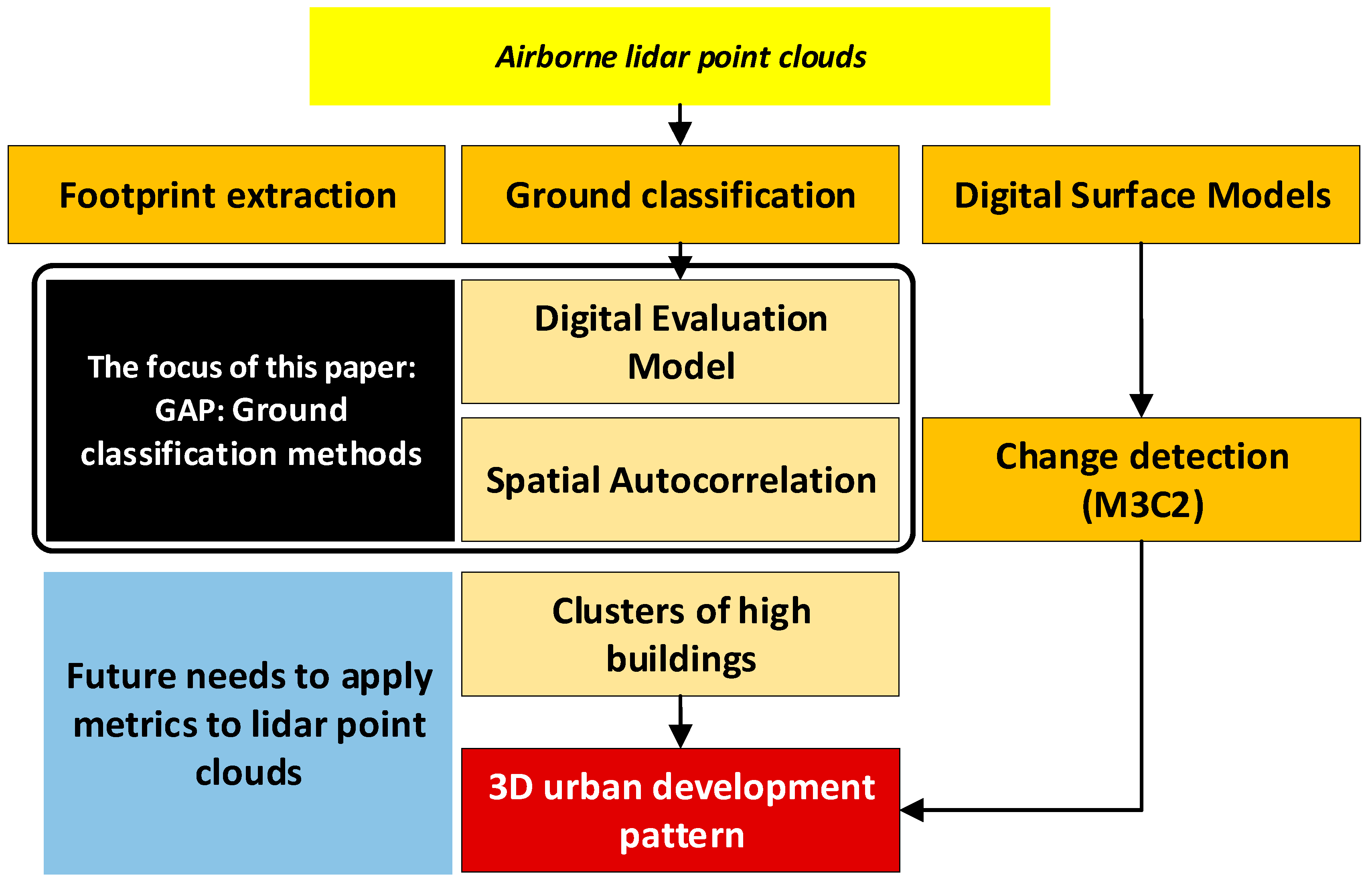
1.2. Gap in Building Heights Metrics Using Temporal Point Cloud in Geographic Information System (GIS)

There is a significant gap in the literature of urban metrics regarding spatial and temporal 3D urban form and change analysis. To fill this gap, appropriate 3D remote-sensing data and urban metrics as well as clear methodologies are required. More specifically, after a thorough review of literature, this work found an important gap in examining different Lidar solutions on difficult terrains such as slant areas. This paper intends to examine a proposed procedure described in the method section on slant areas, which has been overlooked in previous publications. Most of the publications examined flat areas or focused on the roof and other elements of a building [46,60].

The enhanced autocorrelation-based algorithms for Lidar data classification [69] should be applied on different case studies. Empirical analysis of window size, shape, direction and cell size are required in order to assess initial DEM creation, possibility of enhancing the initial DEM, classification of non-ground points and final creation of a normalised digital surface model (NDSM). NDSM includes all nonground points excluding ground elevation. Comparison of the enhanced autocorrelation-based algorithms with existing point-based algorithms in different cases is also an urgent need.

Based on the literature, a set of objectives is designed for identifying both horizontal and vertical dimensions of buildings in an urban environment:

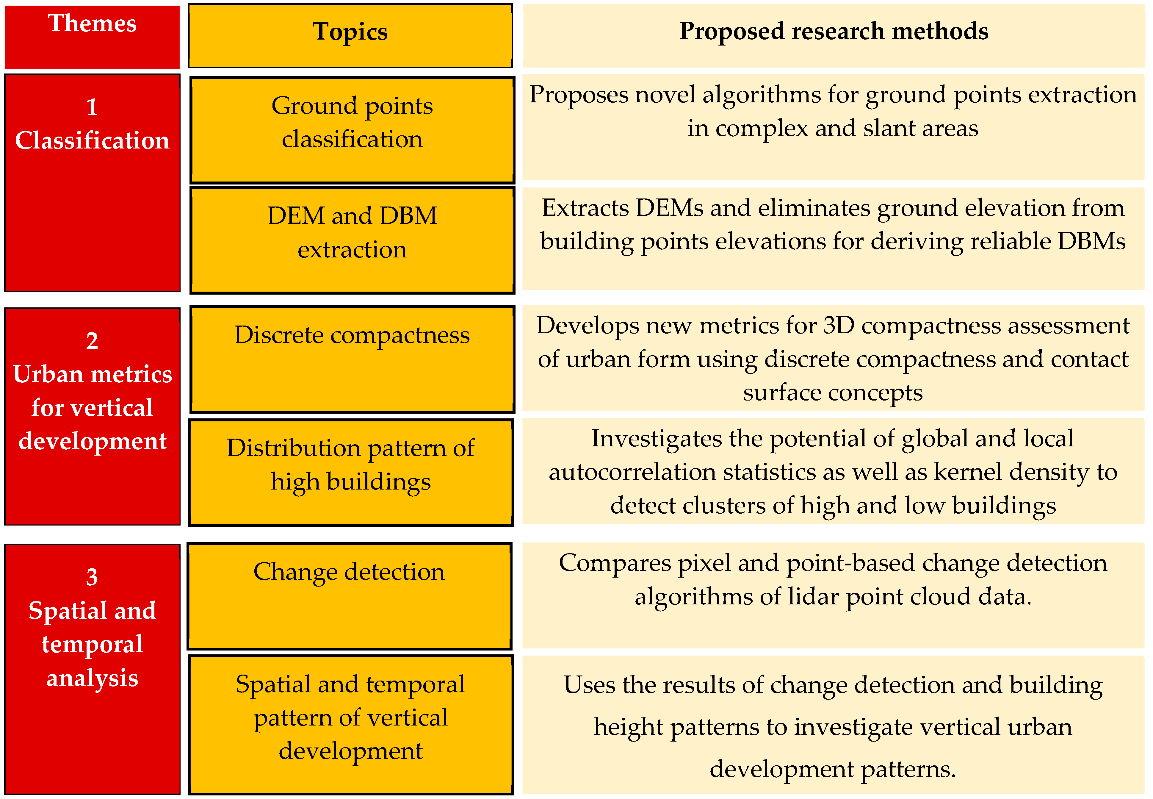
• Objective 1: To propose the application of 3D Discrete Compactness (3D DC), A*, global and local autocorrelation statistics and kernel density in urban block scale for determining the patterns of vertical urban development for extraction of the concentration of relatively higher and lower buildings; and to propose a clear methodology for applying the metrics on height information extracted from remotely sensed 3D data;
• Objective 2: To propose advanced autocorrelation-based algorithms to classify airborne Lidar point cloud data in complex and slant urban areas comprising large buildings, as ground and non-ground points for producing DEM of the terrain surface and NDSM; and to derive the height information of the classified buildings’ points from the extracted DEM and building points’ elevations;
• Objective 3: To investigate the relationship between distribution patterns of concentrated relatively lower and relatively higher buildings to urban structural elements such as major roads; to determine land use types of high buildings for spatial analysis of relationships between different urban objects such as roads and green spaces; and to demonstrate a method for the analysis of spatial and temporal change of 3D urban form.

The listed objectives are part of a procedural framework for building classification, analysing urban 3D forms and measuring urban development by using airborne Lidar data in a GIS environment, and can be used for spatial analysis using a series of Lidar datasets.

Figure 1 lists a summary of these three themes linking to the relevant objectives and proposed methods, which should be considered in order to achieve accurate data of all three dimensions of buildings using airborne Lidar. In this paper, we mainly focus on ground classification as one of the main challenges of processing Lidar data for this research.

2. Research Method

This paper presents the preliminary tests of our proposed method of extraction of ground elevation in slant areas. Figure 2 shows the methodology for identifying 3D urban development patterns, and the focus of this paper, which is highlighted.

2.1. Study Areas

The main materials for this paper are point cloud datasets from selected areas in Sydney, Australia. As Figure 3 and Figure 4 show, the datasets that are used in this paper include:

(i)

International Society for Photogrammetry and Remote Sensing (ISPRS) samples numbers 3 and 11 (https://www.itc.nl/isprs/wgIII-3/filtertest/downloadsites/);

(ii)

First and last pulse (multiple return) airborne Lidar data over University of New South Wales (UNSW) in Sydney, Australia.

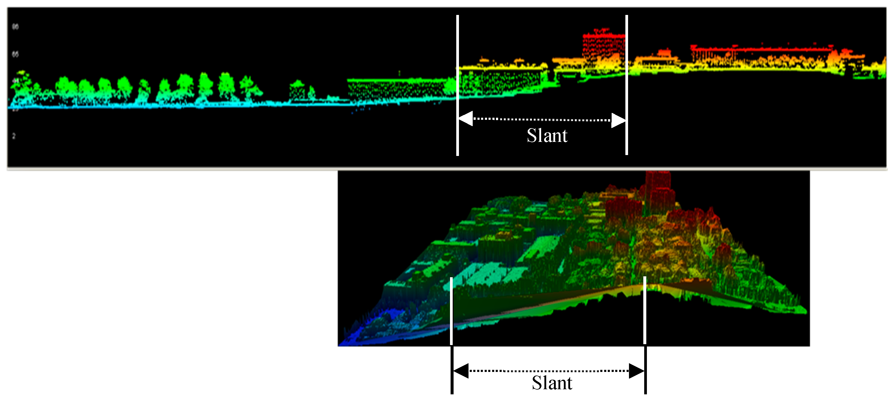
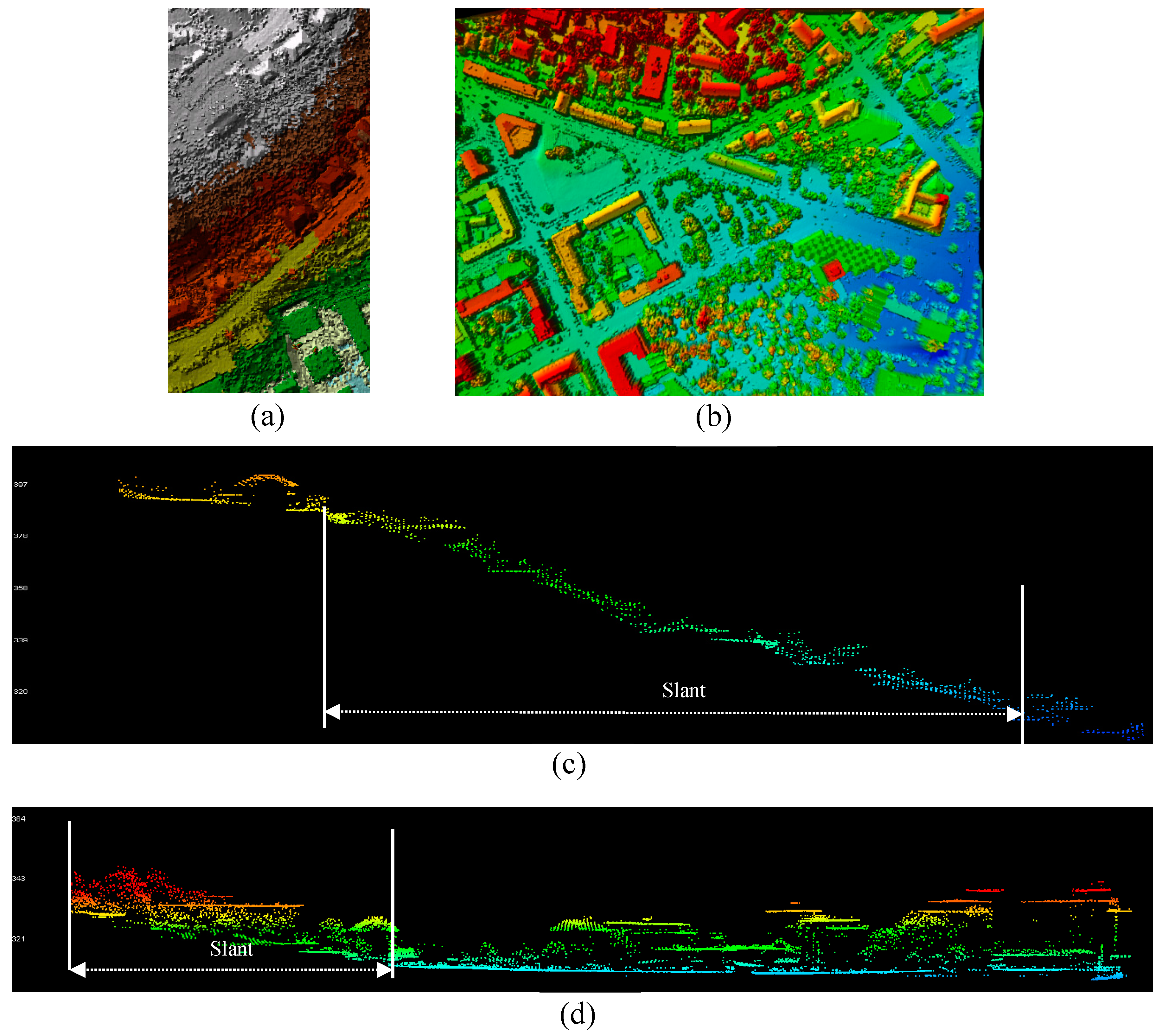
2.2. Digital Elevation Model (DEM) Generation in Slant Areas

The DEMs from Lidar data are generated using classified ground points from point clouds and implementing an appropriate interpolation algorithm such as Natural Neighbour. Hudak, et al. [87] and Meng, et al. [88] and Spaete, et al. [89] present different examples implementing relevant algorithms to Natural Neighbour.

In a preliminary study of the autocorrelation-based algorithms for ground classification [90], omission and commission errors were calculated for validation of the results. We investigated the effect of window size with the same shape on the level of error. In this paper, we explore the effect of window shape and direction on deriving ground points in slant areas and for validation, we calculated kurtosis and skewness of the difference between the reference DEM and our best achieved DEM.

In this method of validation, the values higher and smaller than 2.5 sigma were removed from the histogram. These generated rasters help to understand whether the mean of the differences is close to zero compared to the DEM so better performance of our results can be confirmed and using the measures of skewness and kurtosis, we can answer the question whether the distribution of these differences is close to normal distribution. The histogram is also valuable as it illustrates how the patterns of negative and positive differences are distributed in the raster of the difference.

2.3. Building Footprint Extraction

A pixel-based building classification method using SVM in ENVI software was compared with an object-based method on points using ERDAS software [47]. ArcGIS software is used for data preparation and extraction of building boundaries. The test results on the UNSW dataset using SVM demonstrated significant misclassifications between buildings and roads in sloping terrain. Additionally, careful visual inspection shows acceptable results from an object based classifying tool on the points in ERDAS. Therefore, the object based classifying tool is the choice for building classification and we continued footprint extraction on the results of classified buildings points using ERDAS for time series Lidar data sets in application of 3D urban growth analysis.

Extraction of building boundaries from Lidar data was required for preparing NDSM to be used for grey-level co-occurrence matrix measures and support vector machine classifications in the 3D urban development analysis.

3. Results

3.1. Window Size and Shape Adaptation in Auto-Correlation Based Classification Algorithms

We applied different window sizes and merged the cluster of low elevation values, as ground, and then took minimum points of these clusters to improve the preliminary results. The cell size plays a crucial role in improvement of the results because the mean space of points is 0.8 metres and we have at most two points per square metre. Taking the minimum point out of one or two points would not improve the results as much as required. Whereas, taking minimum points of at most 6 points seems more reasonable, considering the point cloud density and size of objects in the study area. Indeed, this procedure works similarly to a low pass filtering process that removes small objects. Therefore, increasing cell size to 3 m rather than 1m would take minimum points from more low elevation points. These minimum points are utilised for generating our modified DEM.

In the plain area, we extracted the accurate points of large deep areas of ground, by creating a window as large as the plain area. In this way, the ground points in the partially higher area cannot be extracted. These points were extracted by a 100 m square window; however, the points of excavated sites cannot be extracted completely. As a finding, one window size can offset the shortcoming of another window size. Therefore, a combination of window sizescould be helpful but by doing so commission error increases. To minimise the commission error, we generated a raster to obtain minimum elevations from these low points in each 3 m pixel size. The output raster was converted to the point data set in which each cell outputs a point that is representative of minimum value. These new points were used as input of the interpolation algorithm of Inverse Distance Weighted (IDW) to generate 1m-DEM.

In complex areas, all clusters of low values extracted by 100 m, 150 m and 200 m and a window as large as the complex area, were combined and a minimum raster of 3 m cell size was created, then these points were employed in an interpolation step by IDW algorithm to create 1 m-DEM.

In a preliminary study, we tested the effect of shape and size of window in extraction of ground points in a flat area. In addition, the effect of cell size was considered for extraction of a DEM from these ground points. As seen in Figure 5, we firstly extracted the lower points in a window as large as the whole study area. The extracted non-significant points from this step were considered for further application of Local Moran’s I (LMI). A high level of commission error in the lower area was achieved. Therefore, we ignored this step and only kept the ground points from the first step. We also extracted lower points of this study from 100 m window size. While many ground points in the higher area have not been extracted from the application of the large window, the extracted points were enough to fill the gap of the ground points from 100 m window size. Therefore, we merged the points from large and 100 m window size. Then we made a raster of minimum points in every 1, 3, and 5-m cell size and found that the 5 m cell size is more appropriate as it can smooth the ground surface and remove spikes from the DEM. We applied the IDW algorithm of interpolation on the minimum points to generate a DEM. In the last step, we applied a filter of low pass to the DEM to remove the outliers.

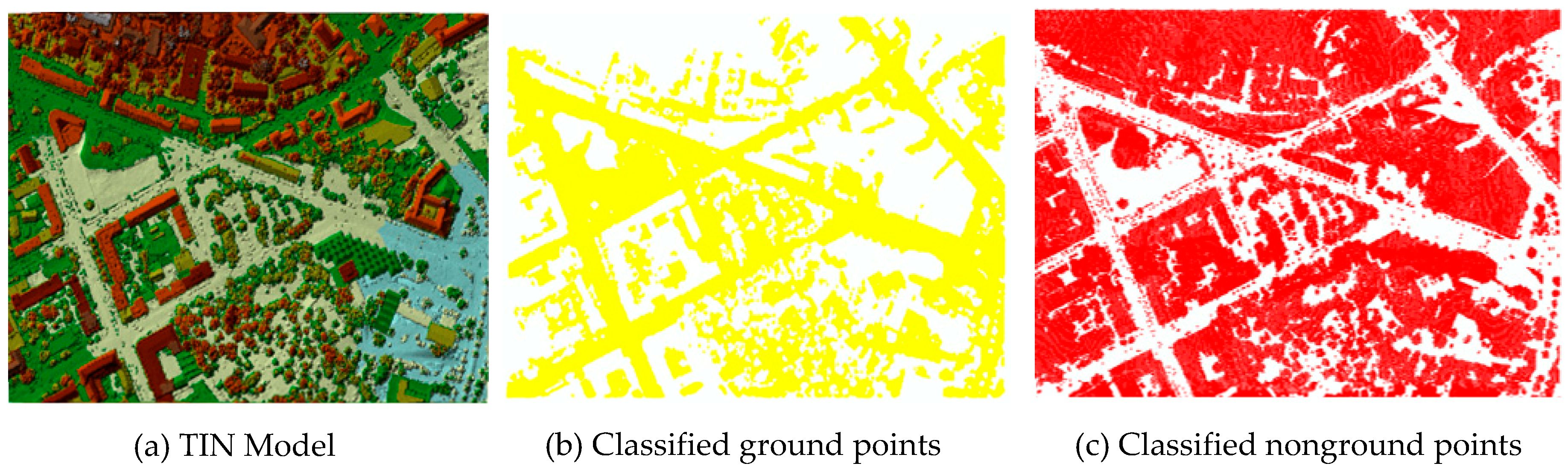
3.2. Effect of Window Shape, Size and Direction on Extraction of Ground Points in Slant Area

We found extraction of ground points in the slant area more challenging and the previous method of extraction ground points in the flat area does not work in the slant area. In the slant area, using 100 m, 150 m and 200 m window sizes and even a moving 100 m window size could not produce proper results for ground points segmentation. As the shape and size of the window are found to be very effective on the results, we started the exploration of extraction of ground points in the slant area in rectangular window shapes. In the slant area, 100 m window size can only detect the lower points and the ground points in higher elevation areas cannot be detected [69]. As the sensitivity of the slant area to the shape and size of the windows was higher than other areas, different rectangular windows 40 m × 490 m, 18 m × 490 m, 25 m × 490, 7 m × 490 m were tested and it was concluded that 7 m × 490 m extracts more ground points. Moreover, the position of these windows against the slope was highly important as they have to be perpendicular to slope vector. The rasterization effect in the slant area was not clear as the 3 m cell size produced a higher commission error. Therefore, 1 m was the optimal cell size for the slant area.

By visual inspection and comparison with the triangulation irregular network (TIN) model of the digital surface model (DSM), we concluded that optimum window size to be adapted with the scene specifications is 7 m × 490 m for our selected sample. The reason behind using narrow and long rectangles parallel to contour lines in slant areas is to increase the possibility of getting ground points out of approximately lower points than average value within a certain distance of neighbouring points in a data set. Figure 6a illustrates a narrow long window. We also found that the direction of these windows has effects on obtaining better results. This means that parallel windows perpendicular on the slope vector direction can extract more ground points. Therefore, a supervised method of thin and long windows perpendicular to the slope vector can improve the correctly classified ground points significantly. Figure 6b demonstrates the extracted ground points by this method that are overlaid to a DSM for better visualisation of the results.

Some studies show that moving windows improves the bare-earth segmentation [91], but in this research, moving windows of 100 m in 1 m stepping distance (see the profiles of each window step in Figure 7) and thin windows increased the commission error.

As the next step, two different configurations of rasterization and DEM cell size have been tested for the slant area. In the first method, the minimum raster of 1 m and a DEM of 5 m was applied. Figure 8 shows the results of 1 m, 3 m and 5 m rasterization in achieved DEM. Figure 9 shows the histogram of the difference between these two DEMs cell by cell. A second configuration of 3 m rasterization and 1m DEM for the slant area was tested. As can be seen in Figure 9, the second method improves the results by pushing the mean closer to zero and obtaining a higher number of pixels’ difference around zero. A high difference occurs where a few ground points have been extracted by LMI in thin windows in using both LMI and Gi* [69] as statistics to extract approximately lower points.

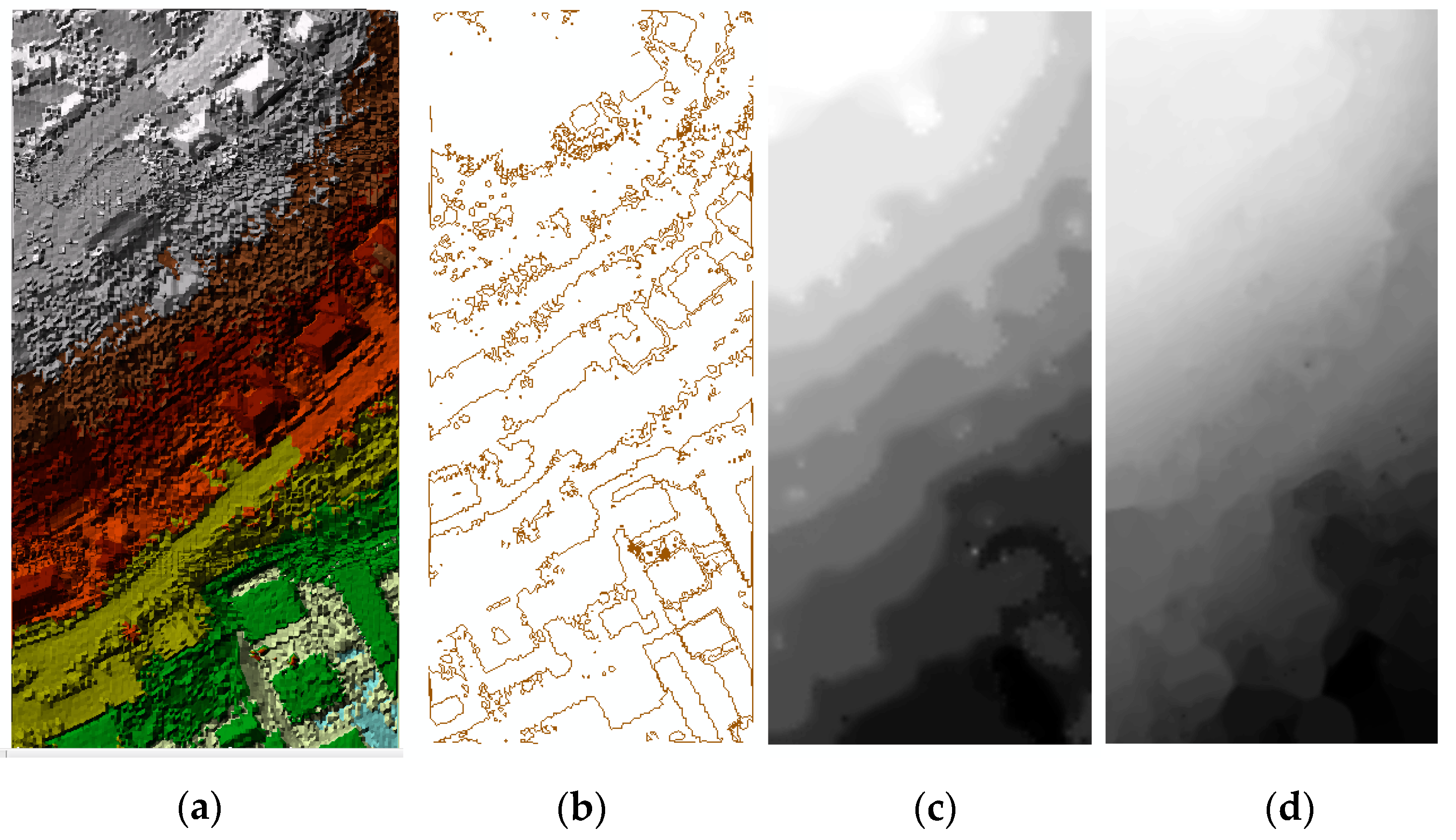
3.3. DEM Extraction Using Contour Lines in Slant Area

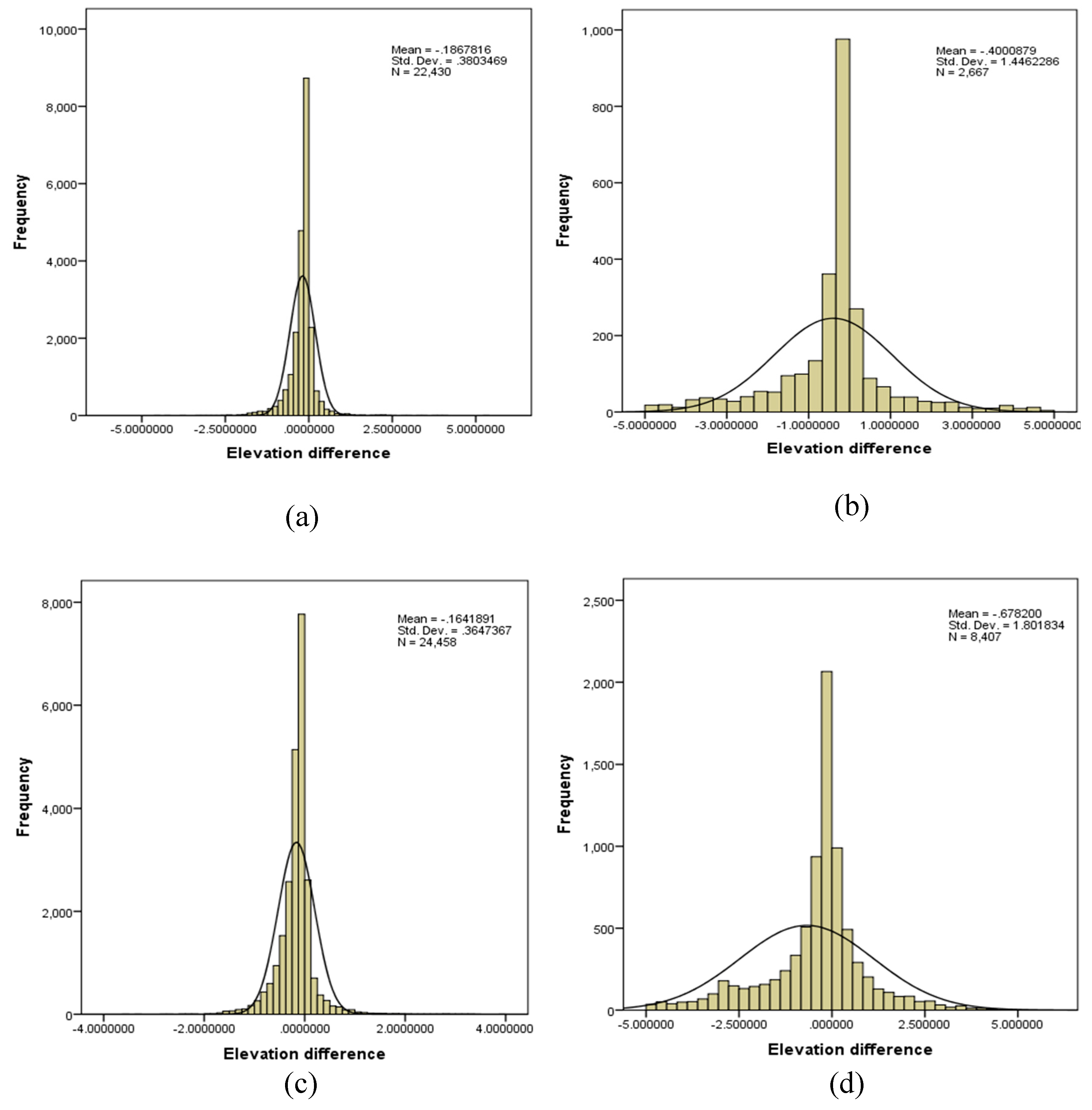
In this method, the DEM is extracted through the following steps. In ISPRS data set, we created a TIN model and generated contour lines from the TIN model using 10m interval as shown in Figure 10b. These contour lines are then used for making a DEM based on their values (see Figure 10c). During this procedure, some of the objects such as buildings and trees are removed. The DEM is used for separation of ground and non-ground points. Any point higher than 1 m from this DEM is considered as a non-ground point and other points as ground points.

For another data set (i.e. ISPRS sample 3), we based this method for separation of ground and non-ground points as seen in Figure 11. These results show that this method still needs improvement for this site.

3.4. Validation

The results show that the method of narrow long windows in the slant area produces better results than the method of contour line as the level of commission error in the slant area using the contour line method is higher than the narrow long window. The results of the achieved DEMs are validated through histograms of the difference between our results and the reference DEM. Two autocorrelation statistics of LMI and Gi* are explored for the extraction of ground points and the skewness and kurtosis of these histograms are calculated to see how similar our results are to the reference DEM.

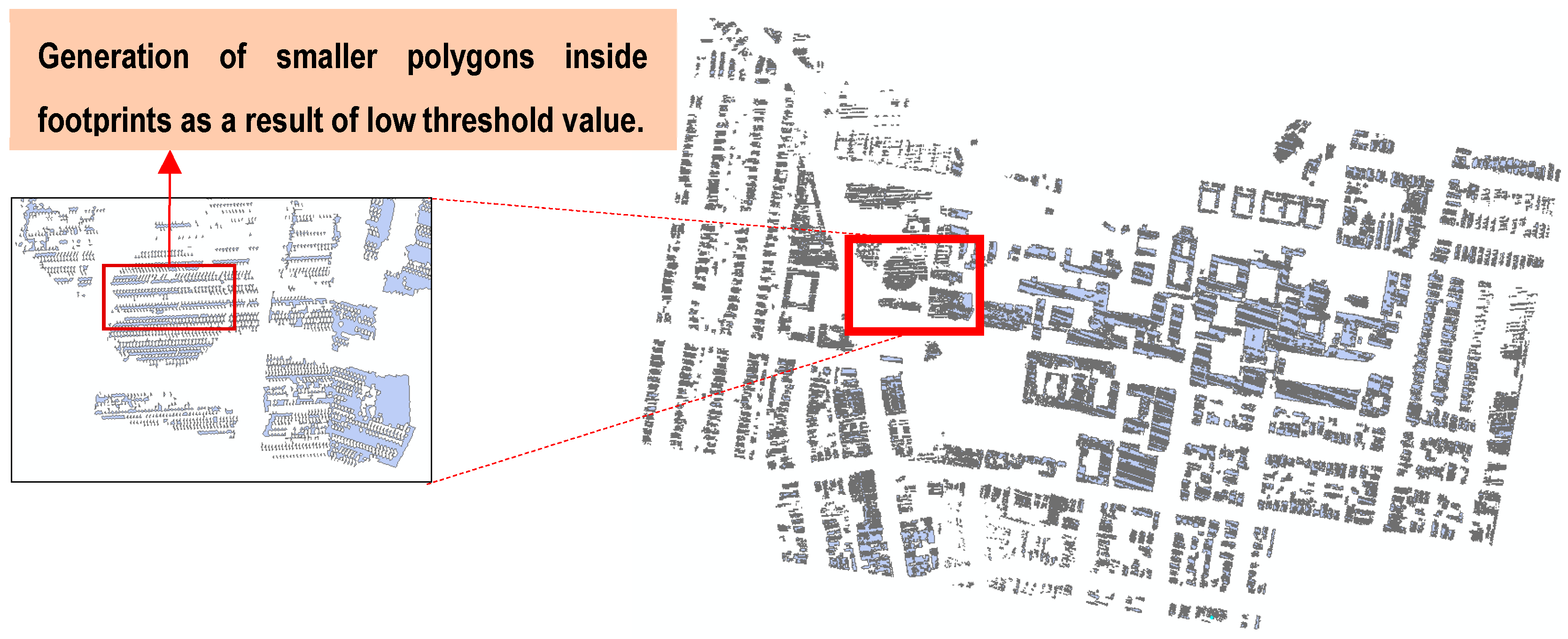
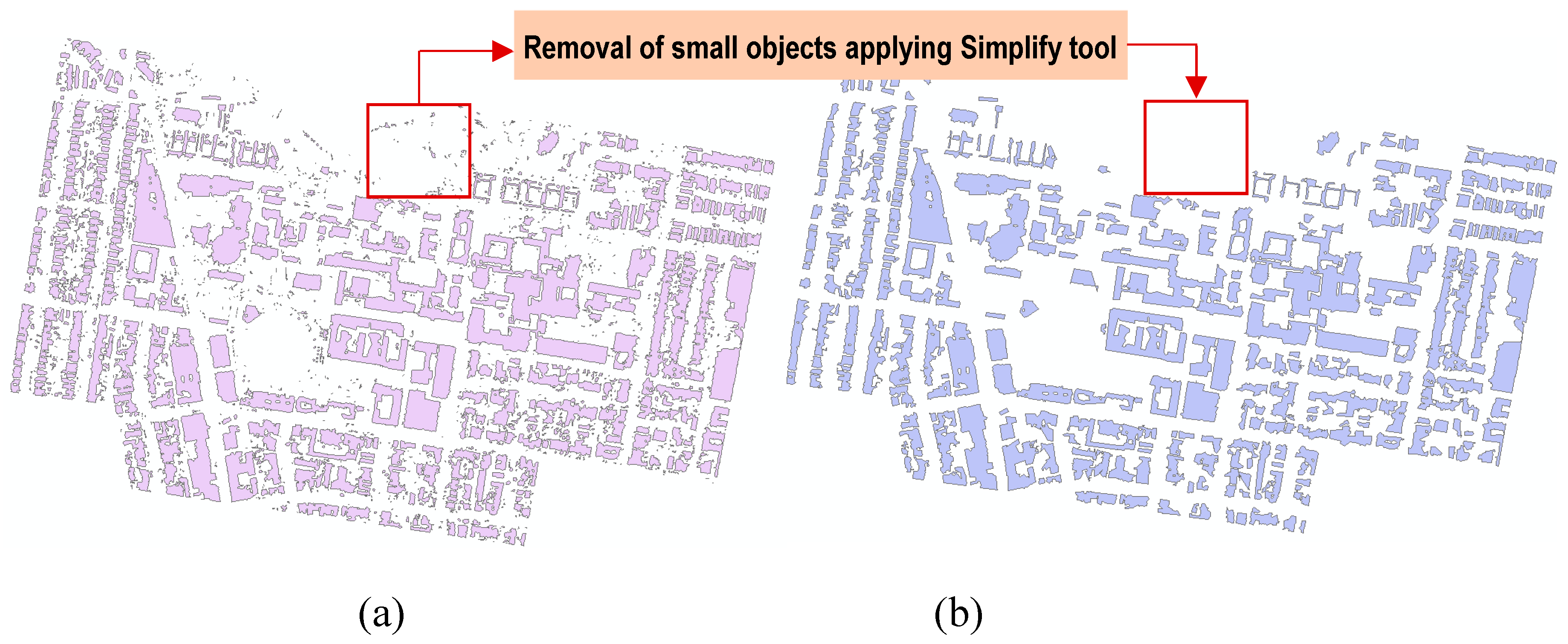
3.5. Buildings Boundaries Extraction

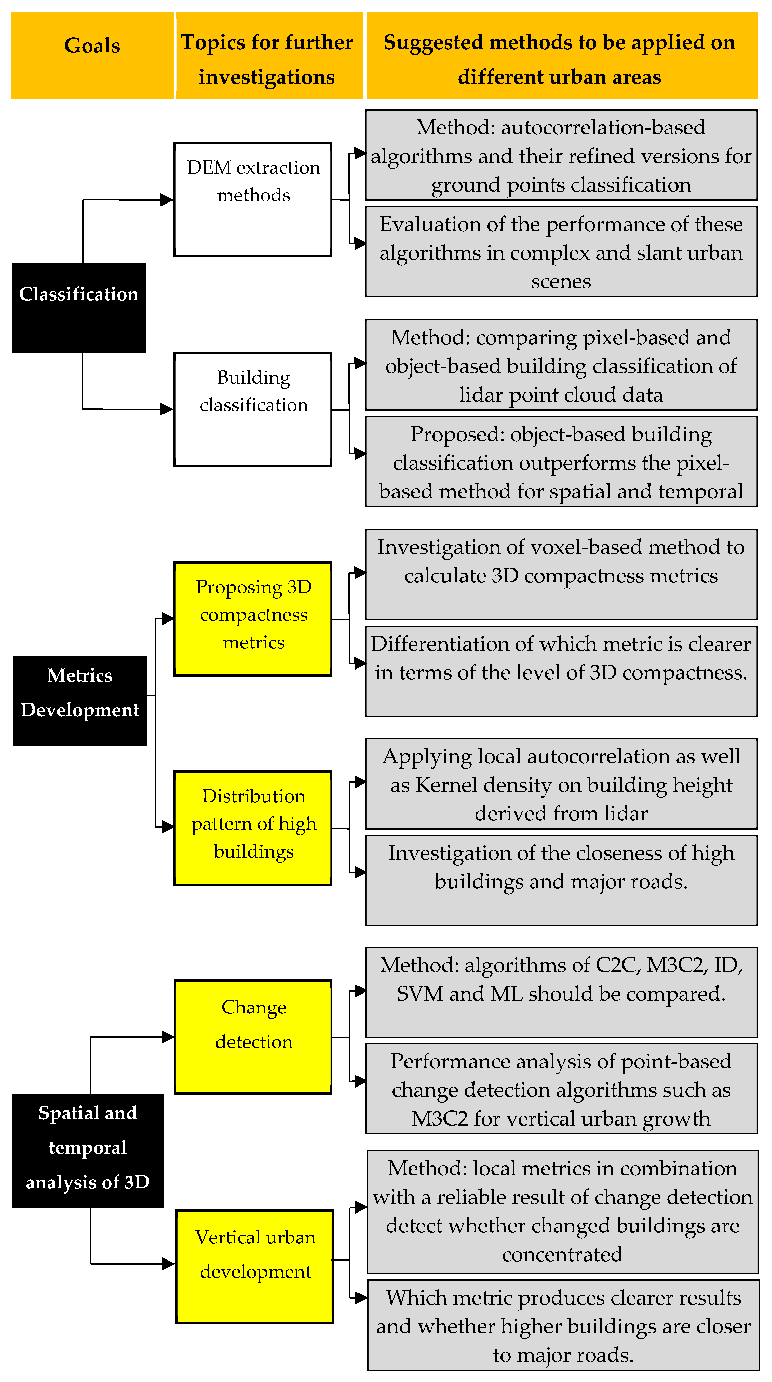
The results of the tests using aggregating points and simplification methods for building boundary extraction in ArcGIS show that a small aggregation distance (e.g., 1.5 m) results in generation of many small polygons for one building as illustrated in Figure 12 and a large threshold causes the joining of separate buildings.

Among tested aggregation distances, an empirical threshold of 2.5 m results in acceptable outcomes. Larger values for the threshold aggregates more than one building in a polygon. Lower values generate small polygons inside footprints (refer to Figure 12). In addition, using the Simplify building tool will remove the small objects with an assigned threshold as shown in Figure 13a,b. Smaller objects with area less than 100 m² were removed from Figure 13b. We suggest conducting this approach for 3D urban growth analysis.

4. Discussion

As using only contour lines cannot omit all the buildings and objects, further processing can be done in future studies to making narrow windows parallel to contour lines in slant areas and then applying LMI and Gi*. Indeed, the combination of these two methods is suggested for future studies. The proposed steps for this new method are: (a) to make narrow windows parallel to contour lines through making a 3 m buffer around the contour lines, (b) to split the buffers to individual polygons, then consider these polygons for application of autocorrelation statistics; (c) to extract clusters of lowest points as ground; (d) to apply slope-based filtering for removing outliers; (e) to generate DEM from the extracted ground points.

This paper focused on slant areas and building classifications, and DEM improvement on complex scenes has been achieved by Shirowzhan, et al. [69]. In Shirowzhan, et al. [69], we found that four parameters of window size, cell size, z-score and p-values of Gi* and LMI spatial statistics affect the results of classification in complex urban scenes. In this paper, we tested the effect of window direction and shape on the results for autocorrelation-based ground classification algorithms and found that the two parameters are important in extraction of ground points in slant areas using both autocorrelation spatial statistics. However, other proposed objectives can be replicated in different case studies examining the discussed methods on different areas with complex geometry and building attributes. Manual or semi-automatic classification provides relatively good results compared to an automatic procedure but these are typically time consuming and challenging in complex and slant areas.

We applied novel autocorrelation-based classification algorithms for classification of ground and non-ground points in slant areas. Minimum-based rasterization and slope-based filtering are suggested to be integrated in the processing in order to effectively remove spikes from the DEMs. The test results showed that these enhanced algorithms produced high-quality overall classification accuracy and assessment based on skewness and kurtosis.

In terms of urban metrics, the authors suggest that 3D DC, A*, global and local autocorrelation statistics and kernel density should be applied in different urban areas such as urban blocks. In addition, global and local autocorrelation statistics (MI, LMI, G_i and G_i*) and kernel density should be applied to airborne Lidar data sets in different urban areas including a wider range of building forms and infrastructure elements in order to explore the patterns of concentration of relatively higher buildings.

This paper highlights the importance of classification algorithms and solving technical problems in a top-down approach for analysing and explaining 3D patterns in urban areas. From a technical perspective, this paper presents new methods for refining autocorrelation-based algorithms in slant areas. By contrast with other studies which focus on flat areas, this paper tackles examining slant areas using point cloud data sets. Methodologically, four main experimentations of window size, window shape, window direction and cell size were chosen and empirically examined to find out how it can improve DEM creation in slant areas. In addition, our experimentation compares building boundaries extraction from classified buildings’ points within a GIS environment.

One of the main implications of investigating ground classifications, building height and urban form analytics is to produce accurate data for buildings, developing robust metrics for detection of the compactness of vertical development and applying all metrics on different data sets. This would help in detecting changes in a smarter way which is required for achieving smart city concepts and improving urban planning models. The ground and non-ground classification algorithms can be used for development of ArcGIS tools in terms of DEM and NDSM extraction from airborne Lidar point cloud data.

There have been barriers in the past on how to investigate 3D patterns of urban form. For exploring the trends of change detection of spatial and temporal urban form, Shirowzhan et al. [47] suggested change detection algorithms, which are important for urban planners to decide which of the existing methods of change detection should be applied. While there are metrics to characterise horizontal patterns of urban fabric, it is challenging to identify vertical patterns of urban fabric due to a lack of reliable height information, methods to model the distribution of building heights, methodologies to detect 3D urban patterns, and spatial analysis methods. Recently, the rate of vertical urban development has created an urgent need for characterising the trends and patterns of these developments. Change detection in building heights for 3D map updating is the first step for monitoring this type of urban development. Repeated airborne Lidar data coverage can provide accurate 3D data revealing a height difference of the buildings over time.

The point and pixel-based change detection algorithms of Lidar data should be compared We suggest comparison of five change detection algorithms for the airborne Lidar data such as support vector machine (SVM), maximum likelihood (ML), image differencing (ID), cloud to cloud (C2C) and multiple model to model cloud comparison (M3C2) [61]. In a spatial and temporal analysis, it is critical to examine the capabilities of Local Moran’s I, G_i* and kernel density in hot spot analysis of building height patterns. Figure 14 highlights the contributions of this research and some avenues for future studies for developing a variety of urban metrics. The drivers and factors influencing 3D patterns and growth of urban areas are required to be identified by urban planners and economists. This study discussed that Lidar solutions can assist in producing the required building height information, hence the following questions should be addressed in different contexts:

• Factors, drivers and processes influencing different types of 3D urban patterns;
• Spatial urban theories and model modifications to consider both urban growth and various vertical patterns;
• Adding 3D DC and A* to the current metrics for urban block-scale analysis [61];
• Applying the global and local autocorrelation statistics as metrics appropriate for different cases of urban areas at the city and block scale; and
• Applying the kernel density appropriate for urban block scale on various cases of different countries.

Figure 14 also shows three categories of urban metrics in different scales of plot, block and city [61]. The proposed local and global autocorrelation statistics for deriving the distribution pattern of heights can be added to the currently available metrics in both urban block and city scales [61]. We suggest comparing a pixel-based building classification method with an object-based classification tool that classifies the points directly. The classified building points in conjunction with the derived DEM were used for extraction of digital building models (DBMs).

This study also suggests that future studies should select different case studies and employ the concepts of contact surface (A*) and 3D DC to measure the level of 3D urban compactness. The replications of the methods will be considered as validation based on simulation data sets and DBMs of urban areas extracted from airborne Lidar data. In the simulation study, using a 3 × 3 matrix of horizontal and vertical urban fabric patterns, nine 3D urban fabric types would be suggested, and the same size urban extents with different typologies can be extracted from the Lidar data. The results from both simulation and 3D point clouds may show the differentiation among the typologies using A* and 3D DC.

Our investigations show the need for describing building height patterns in urban areas to obtain essential information about spatial and temporal vertical development of the urban fabric. The spatial relationship between the patterns of high building points and other urban elements as well as their corresponding land use should be investigated.

The information such as derived patterns of compactness of relatively higher and lower buildings, can be used by developing big data for urban planners and managers for better planning of future directions of development of cities, as well as decisions on the location of relatively higher and lower buildings, with the knowledge of the current developments. Recently, the need for large scale Lidar data and big spatial data are confirmed in the literature [92,93,94,95,96].

Our investigation of spatial and temporal urban form change detection may provide a monitoring technique for urban planners to investigate the trends of vertical urban development at specific time intervals. The information derived from both 3D building and vegetation change detection can be used in a sustainability study for urban forms to explore whether the trends of physical change of 3D urban form is favourable for sustainability in the era of climate change [90]. The need for the applications of Lidar in sustainable development and landscape have been discussed in recent studies such as: Bonczak and Kontokosta [96] in complex urban landscapes; Guo, et al. [97] for modelling habitat connectivity variables to prioritise spatial conservation issues; and Wentz, et al. [98] for addressing dynamics of urban forms in global cities. The research themes presented in this work are fundamentally important for developing ideas such as the 3D space syntax [99] that answers the question of how 3D urban fabric patterns may affect movement patterns, safety, land value [100,101,102].

In addition, high-accuracy DBMs are required for a variety of applications e.g., urban planning and hydrology modelling, civil engineering and surveying. For example, DBMs can be used for footprint extraction and mapping updating purposes. The implication of our findings is in urban morphology studies, since they need DBMs for measuring spatial metrics such as a floor area ratio (FAR) and building coverage ratio (BCR).

In the process of elimination of ground elevation from classified buildings points, we found that in slant areas the geometry of the roof tops changes (See Figure 15). For future research, we suggest investigating how to solve such a problem. This solution would be very important in studies on the estimation of photovoltaic potentials that is influenced by the geometry and slope direction of roof tops as these characteristics affect the level of solar gain. These results are crucial for characterising 3D urban developments over time specifically for the assessment of sustainability of urban form to compute how buildings volumetrically change compared to vegetation in a city.

5. Conclusions

This study aimed to test new methods for refining autocorrelation-based algorithms in slant areas and to compare building boundaries extraction from classified buildings points within a GIS environment. These aims are considered for solving technical problems we have faced in 3D urban growth analyses.

Four parameters, namely window size, window shape and direction, cell size were empirically selected in order to improve the DEM in slant areas. The results show that the presented algorithms in this paper improve DEMs in slant areas. However, these algorithms still need further improvements in such areas. The method utilised in this study is to consider narrow long square windows perpendicular to the slope vector in slant areas with 1 m stepping between the windows’ movements and also to make contour lines with 10 m intervals in slant areas. The novelties in our experiments are: (i) window direction and contour lines for slant area; (ii) applying moving windows; and (iii) iterated non-ground extraction. These approaches produce acceptable results; however, further improvement is proposed for future studies through making buffers around contour lines and considering these buffers as windows that should be perpendicular to the slope vector and can be used for applying spatial autocorrelation statistics such as Local Moran’s I.

The contributions of this paper are the proposition of considering four parameters in autocorrelation-based algorithms for extraction of ground points in slant areas and comparison among the methods of building boundaries’ extraction in the GIS environment. This study showed that the direction of the windows i.e., stretching windows parallel to contour lines and extraction of contour lines with a distance interval improves classification in slant areas.

References

1. Monteiro, C.S.; Costa, C.; Pina, A.; Santos, M.Y.; Ferrão, P. An urban building database (UBD) supporting a smart city information system. Energy Build. 2018, 158, 244–260. [Google Scholar] [CrossRef]
2. Neuville, R.; Pouliot, J.; Poux, F.; de Rudder, L.; Billen, R. A Formalized 3D Geovisualization Illustrated to Selectivity Purpose of Virtual 3D City Model. ISPRS Int. J. Geo-Inf. 2018, 7, 194. [Google Scholar] [CrossRef]
3. Elhoseny, H.; Elhoseny, M.; Riad, A.M.; Hassanien, A.E. A framework for big data analysis in smart cities. In Proceedings of the International Conference on Advanced Machine Learning Technologies and Applications, Cairo, Egypt, 22–24 February 2018; Springer: Cham, Switzerland, 2018; pp. 405–414. [Google Scholar] [CrossRef]
4. Berghauser Pont, M. An Analytical Approach to Urban Form. In Teaching Urban Morphology; Springer: Cham, Switzerland, 26 April 2018; pp. 101–119. [Google Scholar] [CrossRef]
5. Sani, M.J.; Rahman, A.A. GIS and BIM integration at data level: A review. Int. Soc. Photogramm. Remote Sens. 2018, XLII-4/W9, 299–306. [Google Scholar] [CrossRef]
6. Jelokhani-Niaraki, M.; Sadeghi-Niaraki, A.; Choi, S.-M. Semantic interoperability of GIS and MCDA tools for environmental assessment and decision making. Environ. Model. Softw. 2018, 100, 104–122. [Google Scholar] [CrossRef]
7. Hare, T.M.; Rossi, A.P.; Frigeri, A.; Marmo, C. Interoperability in planetary research for geospatial data analysis. Planet. Space Sci. 2018, 150, 36–42. [Google Scholar] [CrossRef] [Green Version]
8. Li, X.; Cheng, S.; Lv, Z.; Song, H.; Jia, T.; Lu, N. Data analytics of urban fabric metrics for smart cities. Future Gener. Comput. Syst. 2018, in press. [Google Scholar] [CrossRef]
9. Jing, Y.; Liu, Y.; Cai, E.; Yi, L.; Zhang, Y. Quantifying the spatiality of urban leisure venues in Wuhan, Central China–GIS-based spatial pattern metrics. Sustain. Cities Soc. 2018, 40, 638–647. [Google Scholar] [CrossRef]
10. Rejeb Bouzgarrou, A.; Claramunt, C.; Rejeb, H. Visualizing urban sprawl effects of a Tunisian city: A new urban spatial configuration of Monastir. Ann. GIS 2019, 25, 71–82. [Google Scholar] [CrossRef]
11. Corbusier, L.; Etchells, F. Towards a New Architecture. Translated by Frederick Etchells; Dover Publications Inc.: New York, NY, USA, 1946; ISBN 10 0486250237. [Google Scholar]
12. Corbusier, L. The City of To-Morrow and Its Planning; Courier Corporation: North Chelmsford, MA, USA, 1987. [Google Scholar]
13. Machimura, T. The urban restructuring process in Tokyo in the 1980s: Transforming Tokyo into a world city. Int. J. Urban Reg. Res. 1992, 16, 114–128. [Google Scholar] [CrossRef]
14. Beaverstock, J.V.; Smith, R.G.; Taylor, P.J. World-city network: A new metageography? Ann. Assoc. Am. Geogr. 2000, 90, 123–134. [Google Scholar] [CrossRef]
15. Pires, M. Watershed protection for a world city: The case of New York. Land Use Policy 2004, 21, 161–175. [Google Scholar] [CrossRef]
16. Tsutsumi, J. Vertical Extension Processes and Urban Restructuring in Sydney, Australia. In Urban Transformations: Centres, Peripheries and Systems; Routledge: New York, NY, USA, 2016; p. 121. [Google Scholar]
17. Handayani, H.; Murayama, Y.; Ranagalage, M.; Liu, F.; Dissanayake, D. Geospatial analysis of horizontal and vertical urban expansion using multi-spatial resolution data: A case study of Surabaya, Indonesia. Remote Sens. 2018, 10, 1599. [Google Scholar] [CrossRef]
18. Lin, J.; Huang, B.; Chen, M.; Huang, Z. Modeling urban vertical growth using cellular automata—Guangzhou as a case study. Appl. Geogr. 2014, 53, 172–186. [Google Scholar] [CrossRef]
19. Burton, E.; Jenks, M.; Williams, K. Achieving Sustainable Urban Form; Routledge: New York, NY, USA, 2013. [Google Scholar]
20. Jenks, M. Achieving Sustainable Urban Form; Taylor & Francis: London, UK, 2000. [Google Scholar] [CrossRef]
21. Burgess, R.; Jenks, M. Compact Cities: Sustainable urban Forms for Developing Countries; Routledge: New York, NY, USA, 2002. [Google Scholar]
22. Ganser, R.; Williams, K. Brownfield development: Are we using the right targets? Evidence from England and Germany. Eur. Plan. Stud. 2007, 15, 603–622. [Google Scholar] [CrossRef]
23. Office of Deputy Prime Minister. Planning Policy Statement 1: Delivering Sustainable Development; ODPM: London, UK, 2005.
24. Adams, D. The Changing Regulatory Environment for Speculative Housebuilding and the Construction of Core Competencies for Brownfleld Development. Environ. Plan. A 2004, 36, 601–624. [Google Scholar] [CrossRef]
25. Raco, M.; Henderson, S. Sustainable urban planning and the brownfield development process in the United Kingdom: Lessons from the Thames Gateway. Local Environ. 2006, 11, 499–513. [Google Scholar] [CrossRef]
26. Gill, M.; Bhide, A. Densification through vertical resettlement as a tool for sustainable urban development. In Proceedings of the Sixth Urban Research and Knowledge Symposium, Barcelona, Spain, 8–10 October 2012. [Google Scholar]
27. Seraj, T.; Alam, M.S. Housing Problem and Apartment Development in Dhaka City, Dhaka: Past Present Future; The Asiatic Society of Bangladesh: Dhaka, Bangladesh, 2009. [Google Scholar]
28. Wong, K.G. Vertical cities as a solution for land scarcity: The tallest public housing development in Singapore. Urban Des. Int. 2004, 9, 17–30. [Google Scholar] [CrossRef]
29. Lau, S.S.Y.; Giridharan, R.; Ganesan, S. Multiple and intensive land use: Case studies in Hong Kong. Habitat Int. 2005, 29, 527–546. [Google Scholar] [CrossRef]
30. Wang, M.-S.; Chien, H.-T. Environmental behaviour analysis of high-rise building areas in Taiwan. Build. Environ. 1998, 34, 85–93. [Google Scholar] [CrossRef]
31. Chau, K.-W.; Wong, S.K.; Yau, Y.; Yeung, A. Determining optimal building height. Urban Stud. 2007, 44, 591–607. [Google Scholar] [CrossRef]
32. Yu, B.; Liu, H.; Wu, J.; Hu, Y.; Zhang, L. Automated derivation of urban building density information using airborne lidar data and object-based method. Landsc. Urban Plan. 2010, 98, 210–219. [Google Scholar] [CrossRef]
33. Shi, L.; Shao, G.; Cui, S.; Li, X.; Lin, T.; Yin, K.; Zhao, J. Urban three-dimensional expansion and its driving forces—A case study of Shanghai, China. Chin. Geogr. Sci. 2009, 19, 291–298. [Google Scholar] [CrossRef]
34. Lu, Y.; Coops, N.C.; Hermosilla, T. Regional assessment of pan-Pacific urban environments over 25 years using annual gap free Landsat data. Int. J. Appl. Earth Obs. Geoinform. 2016, 50, 198–210. [Google Scholar] [CrossRef]
35. Herold, M.; Menz, G. Landscape metric signatures (LMS) to improve urban land use information derived from remotely sensed data. In A Decade of Trans-European Remote Sensing Cooperation; A A Balkema Publishers: Rotterdam, The Netherlands, 2001; pp. 251–256. ISBN 9789058091871. [Google Scholar]
36. Herold, M.; Goldstein, N.C.; Clarke, K.C. The spatiotemporal form of urban growth: Measurement, analysis and modeling. Remote Sens. Environ. 2003, 86, 286–302. [Google Scholar] [CrossRef]
37. Dietzel, C.; Herold, M.; Hemphill, J.J.; Clarke, K.C. Spatio-temporal dynamics in California’s Central Valley: Empirical links to urban theory. Int. J. Geogr. Inf. Sci. 2005, 19, 175–195. [Google Scholar] [CrossRef]
38. Murayama, Y.; Thapa, R.B. Spatial analysis: Evolution, methods, and applications. In Spatial Analysis and Modeling in Geographical Transformation Process; Springer: Dordrecht, The Netherlands, 2011; pp. 1–26. ISBN 978-94-007-0671-2. [Google Scholar] [CrossRef]
39. Zhao, Y.; Murayama, Y. Urban dynamics analysis using spatial metrics geosimulation. In Spatial Analysis and Modeling in Geographical Transformation Process; Springer: Dordrecht, The Netherlands, 2011; pp. 153–167. ISBN 978-94-007-0670-5. [Google Scholar] [CrossRef]
40. Plowright, A.; Tortini, R.; Coops, N.C. Determining Optimal Video Length for the Estimation of Building Height through Radial Displacement Measurement from Space. ISPRS Int. J. Geo-Inf. 2018, 7, 380. [Google Scholar] [CrossRef]
41. Jat, M.K.; Garg, P.K.; Khare, D. Monitoring and modelling of urban sprawl using remote sensing and GIS techniques. Int. J. Appl. Earth Obs. Geoinform. 2008, 10, 26–43. [Google Scholar] [CrossRef]
42. Bhatta, B.; Saraswati, S.; Bandyopadhyay, D. Quantifying the degree-of-freedom, degree-of-sprawl, and degree-of-goodness of urban growth from remote sensing data. Appl. Geogr. 2010, 30, 96–111. [Google Scholar] [CrossRef]
43. Bhatta, B.; Saraswati, S.; Bandyopadhyay, D. Urban sprawl measurement from remote sensing data. Appl. Geogr. 2010, 30, 731–740. [Google Scholar] [CrossRef]
44. Jaeger, J.A.; Schwick, C. Improving the measurement of urban sprawl: Weighted Urban Proliferation (WUP) and its application to Switzerland. Ecol. Indic. 2014, 38, 294–308. [Google Scholar] [CrossRef]
45. Stathakis, D.; Faraslis, I. Monitoring urban sprawl using simulated PROBA-V data. Int. J. Remote Sens. 2014, 35, 2731–2743. [Google Scholar] [CrossRef]
46. Huang, Y.; Zhuo, L.; Tao, H.; Shi, Q.; Liu, K. A Novel Building Type Classification Scheme Based on Integrated LiDAR and High-Resolution Images. Remote Sens. 2017, 9, 679. [Google Scholar] [CrossRef]
47. Shirowzhan, S.; Trinder, J. Building classification from lidar data for spatio-temporal assessment of 3D urban developments. Procedia Eng. 2017, 180, 1453–1461. [Google Scholar] [CrossRef]
48. Kakon, A.N.; Mishima, N.; Kojima, S. Simulation of the urban thermal comfort in a high density tropical city: Analysis of the proposed urban construction rules for Dhaka, Bangladesh. In Building Simulation; Tsinghua University Press: Beijing, China; Springer: Berlin/Heidelberg, Germany, 2009; Volume 2, p. 291. ISSN 1996-3599. [Google Scholar] [CrossRef]
49. Stewart, I.D.; Oke, T.R. Local climate zones for urban temperature studies. Bull. Am. Meteorol. Soc. 2012, 93, 1879–1900. [Google Scholar] [CrossRef]
50. Irger, M. The Effect of Urban Form on Urban Microclimate. Ph.D. Thesis, Faculty of Built Environment, The University of New South Wales, Sydney, Australia, 2014. [Google Scholar]
51. Giridharan, R.; Ganesan, S.; Lau, S. Daytime urban heat island effect in high-rise and high-density residential developments in Hong Kong. Energy Build. 2004, 36, 525–534. [Google Scholar] [CrossRef]
52. Giridharan, R.; Lau, S.; Ganesan, S.; Givoni, B. Urban design factors influencing heat island intensity in high-rise high-density environments of Hong Kong. Build. Environ. 2007, 42, 3669–3684. [Google Scholar] [CrossRef]
53. Giridharan, R.; Lau, S.; Ganesan, S.; Givoni, B. Lowering the outdoor temperature in high-rise high-density residential developments of coastal Hong Kong: The vegetation influence. Build. Environ. 2008, 43, 1583–1595. [Google Scholar] [CrossRef]
54. Kolokotroni, M.; Giridharan, R. Urban heat island intensity in London: An investigation of the impact of physical characteristics on changes in outdoor air temperature during summer. Sol. Energy 2008, 82, 986–998. [Google Scholar] [CrossRef] [Green Version]
55. Ayata, T. Investigation of building height and roof effect on the air velocity and pressure distribution around the detached houses in Turkey. Appl. Therm. Eng. 2009, 29, 1752–1758. [Google Scholar] [CrossRef]
56. Kotthaus, S.; Grimmond, C.S.B. Energy exchange in a dense urban environment–Part I: Temporal variability of long-term observations in central London. Urban Clim. 2014, 10, 261–280. [Google Scholar] [CrossRef]
57. Murray, A.T.; McGuffog, I.; Western, J.S.; Mullins, P. Exploratory spatial data analysis techniques for examining urban crime: Implications for evaluating treatment. Br. J. Criminol. 2001, 41, 309–329. [Google Scholar] [CrossRef]
58. Hirota, Y.; Izumikawa, H.; Ono, C. Outdoor-to-indoor radio propagation characteristics with 800 MHz band in an urban environment. In Proceedings of the 2014 IEEE Antennas and Propagation Society International Symposium (APSURSI), Memphis, TN, USA, 6–11 July 2014; pp. 697–698. [Google Scholar] [CrossRef]
59. Peifeng, Z.; Yuanman, H.; Hongshi, H. The spatial pattern of building height in Tiexi District. In Proceedings of the 2011 International Conference on Electric Technology and Civil Engineering (ICETCE), Lushan, China, 22–24 April 2011; pp. 1774–1777. [Google Scholar]
60. Gooding, J.; Crook, R.; Tomlin, A.S. Modelling of roof geometries from low-resolution LiDAR data for city-scale solar energy applications using a neighbouring buildings method. Appl. Energy 2015, 148, 93–104. [Google Scholar] [CrossRef] [Green Version]
61. Shirowzhan, S.; Sepasgozar, S.M.E.; Li, H.; Trinder, J. Spatial compactness metrics and Constrained Voxel Automata development for analyzing 3D densification and applying to point clouds: A synthetic review. Autom. Constr. 2018, 96, 236–249. [Google Scholar] [CrossRef]
62. Galster, G.; Hanson, R.; Ratcliffe, M.R.; Wolman, H.; Coleman, S.; Freihage, J. Wrestling sprawl to the ground: Defining and measuring an elusive concept. Hous. Policy Debate 2001, 12, 681–717. [Google Scholar] [CrossRef]
63. Massey, D.S.; Denton, N.A. The dimensions of residential segregation. Soc. Forces 1988, 67, 281–315. [Google Scholar] [CrossRef]
64. Huang, J.; Lu, X.X.; Sellers, J.M. A global comparative analysis of urban form: Applying spatial metrics and remote sensing. Landsc. Urban Plan. 2007, 82, 184–197. [Google Scholar] [CrossRef]
65. Arribas-Bel, D.; Nijkamp, P.; Scholten, H. Multidimensional urban sprawl in Europe: A self-organizing map approach. Comput. Environ. Urban Syst. 2011, 35, 263–275. [Google Scholar] [CrossRef] [Green Version]
66. Kumar, J.A.V.; Pathan, S.; Bhanderi, R. Spatio-temporal analysis for monitoring urban growth–a case study of Indore city. J. Indian Soc. Remote Sens. 2007, 35, 11–20. [Google Scholar] [CrossRef]
67. Massam, B.H.; Goodchild, M.F. Temporal trends in the spatial organization of a service agency. Can. Geogr./Le Géographe Canadien 1971, 15, 193–206. [Google Scholar] [CrossRef]
68. Angel, S.; Parent, J.; Civco, D. Urban sprawl metrics: An analysis of global urban expansion using GIS. In Proceedings of the ASPRS 2007 Annual Conference, Tampa, FL, USA, 7–11 May 2007. [Google Scholar]
69. Shirowzhan, S.; Lim, S.; Trinder, J. Enhanced autocorrelation-based algorithms for filtering airborne lidar data over urban areas. J. Surv. Eng. 2016, 142, 04015008. [Google Scholar] [CrossRef]
70. Sreevalsan-Nair, J. Visual Analytics of Three-Dimensional Airborne LiDAR Point Clouds in Urban Regions. In Geospatial Infrastructure, Applications and Technologies: India Case Studies; Springer Nature Singapore Pte Ltd.: Singapore, 2018; pp. 313–325. [Google Scholar]
71. Rosser, J.F.; Boyd, D.S.; Long, G.; Zakhary, S.; Mao, Y.; Robinson, D. Predicting residential building age from map data. Comput. Environ. Urban Syst. 2019, 73, 56–67. [Google Scholar] [CrossRef]
72. Sepasgozar, S.M.E.; Forsythe, P.; Shirowzhan, S. Evaluation of terrestrial and mobile scanner technologies for part-built information modeling. J. Constr. Eng. Manag. 2018, 144, 04018110. [Google Scholar] [CrossRef]
73. Sepasgozar, S.; Shirowzhan, S.; Wang, C.C. A Scanner Technology Acceptance Model for Construction Projects. Procedia Eng. 2017, 1237–1246. [Google Scholar] [CrossRef]
74. Sepasgozar, S.M.; Forsythe, P.; Shirowzhan, S.; Norzahari, F. Scanners And Photography: A Combined Framework. In Proceedings of the 40th Australasian Universities Building Education Association (AUBEA) 2016 Conference, Cairns, Australia, 6–8 July 2016; pp. 819–828. [Google Scholar]
75. Sepasgozar, S.M.E.; Lim, S.; Shirowzhan, S.; Kim, Y.M. Implementation of As-Built Information Modelling Using Mobile and Terrestrial Lidar Systems. In Proceedings of the 31st International Symposium on Automation and Robotics in Construction and Mining (ISARC 2014), Sydney, Australia, 9–11 July 2014. [Google Scholar]
76. Sepasgozar, S.M.; Lim, S.; Shirowzhan, S. Implementation of Rapid As-built Building Information Modeling Using Mobile LiDAR. In Proceedings of the Construction Research Congress 2014, Construction in a Global Network, Atlanta, GA, USA, 19–21 May 2014; pp. 209–218, ISBN 9780784413517. [Google Scholar]
77. Shirowzhan, S.; Sepasgozar, S.; Liu, C. Monitoring physical progress of indoor buildings using mobile and terrestrial point clouds. In Proceedings of the Construction Research Congress 2018, Construction Research Congress 2018, New Orleans, LA, USA, 2–4 April 2018. [Google Scholar] [CrossRef]
78. Goldbergs, G.; Levick, S.R.; Lawes, M.; Edwards, A. Hierarchical integration of individual tree and area-based approaches for savanna biomass uncertainty estimation from airborne LiDAR. Remote Sens. Environ. 2018, 205, 141–150. [Google Scholar] [CrossRef]
79. Xu, Q.; Man, A.; Fredrickson, M.; Hou, Z.; Pitkänen, J.; Wing, B.; Ramirez, C.; Li, B.; Greenberg, J.A. Quantification of uncertainty in aboveground biomass estimates derived from small-footprint airborne LiDAR. Remote Sens. Environ. 2018, 216, 514–528. [Google Scholar] [CrossRef]
80. Jaboyedoff, M.; Oppikofer, T.; Abellán, A.; Derron, M.-H.; Loye, A.; Metzger, R.; Pedrazzini, A. Use of LIDAR in landslide investigations: A review. Nat. Hazards 2012, 61, 5–28. [Google Scholar] [CrossRef]
81. Bossi, G.; Cavalli, M.; Crema, S.; Frigerio, S.; Quan Luna, B.; Mantovani, M.; Marcato, G.; Schenato, L.; Pasuto, A. Multi-temporal LiDAR-DTMs as a tool for modelling a complex landslide: A case study in the Rotolon catchment (eastern Italian Alps). Nat. Hazards Earth Syst. Sci. 2015, 15, 715–722. [Google Scholar] [CrossRef]
82. Bitelli, G.; Conte, P.; Csoknyai, T.; Mandanici, E. Urban energetics applications and Geomatic technologies in a Smart City perspective. Int. Rev. Appl. Sci. Eng. 2015, 6, 19–29. [Google Scholar] [CrossRef]
83. Hu, M.; Li, C. Design smart city based on 3S, internet of things, grid computing and cloud computing technology. In Internet of Things; Springer: Berlin/Heidelberg, Germany, 2012; pp. 466–472. [Google Scholar] [CrossRef]
84. Lohani, B.; Ghosh, S. Airborne LiDAR Technology: A Review of Data Collection and Processing Systems. Proc. Natl. Acad. Sci. India Sect. A Phys. Sci. 2017, 87, 567–579. [Google Scholar] [CrossRef]
85. Reutebuch, S.E.; McGaughey, R.J.; Andersen, H.-E.; Carson, W.W. Accuracy of a high-resolution lidar terrain model under a conifer forest canopy. Can. J. Remote Sens. 2003, 29, 527–535. [Google Scholar] [CrossRef] [Green Version]
86. Mennis, J.; Guo, D. Spatial data mining and geographic knowledge discovery: An introduction. Comput. Environ. Urban Syst. 2009, 33, 403–408. [Google Scholar] [CrossRef]
87. Hudak, A.T.; Crookston, N.L.; Evans, J.S.; Hall, D.E.; Falkowski, M.J. Nearest neighbor imputation of species-level, plot-scale forest structure attributes from LiDAR data. Remote Sens. Environ. 2008, 112, 2232–2245. [Google Scholar] [CrossRef]
88. Meng, X.; Currit, N.; Zhao, K. Ground Filtering Algorithms for Airborne LiDAR Data: A Review of Critical Issues. Remote Sens. 2010, 2, 833–860. [Google Scholar] [CrossRef] [Green Version]
89. Spaete, L.P.; Glenn, N.F.; Derryberry, D.R.; Sankey, T.T.; Mitchell, J.J.; Hardegree, S.P. Vegetation and slope effects on accuracy of a LiDAR-derived DEM in the sagebrush steppe. Remote Sens. Lett. 2011, 2, 317–326. [Google Scholar] [CrossRef]
90. Shirowzhan, S.; Lim, S. Autocorrelation statistics-based algorithms for automatic ground and non-ground classification of Lidar data. In Proceedings of the International Symposium on Automation and Robotics in Construction (ISARC), Sydney, Australia, 9–11 July 2014; Volume 31, p. 1. [Google Scholar]
91. Su, W.; Sun, Z.; Zhong, R.; Huang, J.; Li, M.; Zhu, J.; Zhang, K.; Wu, H.; Zhu, D. A new hierarchical moving curve-fitting algorithm for filtering lidar data for automatic DTM generation. Int. J. Remote Sens. 2015, 36, 3616–3635. [Google Scholar] [CrossRef]
92. Li, Z.; Hodgson, M.E.; Li, W. A general-purpose framework for parallel processing of large-scale LiDAR data. Int. J. Dig. Earth 2018, 11, 26–47. [Google Scholar] [CrossRef]
93. Evans, M.R.; Oliver, D.; Yang, K.; Zhou, X.; Ali, R.Y.; Shekhar, S. Enabling spatial big data via CyberGIS: Challenges and opportunities. In CyberGIS for Geospatial Discovery and Innovation; Springer: Dordrecht, The Netherlands, 2019; pp. 143–170. [Google Scholar]
94. Zheng, M.; Tang, W.; Lan, Y.; Zhao, X.; Jia, M.; Allan, C.; Trettin, C. Parallel Generation of Very High Resolution Digital Elevation Models: High-Performance Computing for Big Spatial Data Analysis. In Big Data in Engineering Applications; Springer Nature Singapore Pte Ltd.: Singapore, 2018; pp. 21–39. [Google Scholar]
95. Bivand, R.; Krivoruchko, K. Big data sampling and spatial analysis: “which of the two ladles, of fig-wood or gold, is appropriate to the soup and the pot?”. Stat. Probab. Lett. 2018, 136, 87–91. [Google Scholar] [CrossRef]
96. Bonczak, B.; Kontokosta, C.E. Large-scale parameterization of 3D building morphology in complex urban landscapes using aerial LiDAR and city administrative data. Comput. Environ. Urban Syst. 2019, 73, 126–142. [Google Scholar] [CrossRef]
97. Guo, X.; Coops, N.C.; Gergel, S.E.; Bater, C.W.; Nielsen, S.E.; Stadt, J.J.; Drever, M. Integrating airborne lidar and satellite imagery to model habitat connectivity dynamics for spatial conservation prioritization. Landsc. Ecol. 2018, 33, 491–511. [Google Scholar] [CrossRef]
98. Wentz, E.A.; York, A.M.; Alberti, M.; Conrow, L.; Fischer, H.; Inostroza, L.; Jantz, C.; Pickett, S.T.A.; Seto, K.C.; Taubenböck, H. Six fundamental aspects for conceptualizing multidimensional urban form: A spatial mapping perspective. Landsc. Urban Plan. 2018, 179, 55–62. [Google Scholar] [CrossRef]
99. Kim, G.; Kim, A.; Kim, Y. A new 3D space syntax metric based on 3D isovist capture in urban space using remote sensing technology. Comput. Environ. Urban Syst. 2019, 74, 74–87. [Google Scholar] [CrossRef]
100. Cooper, H.M.; Chen, Q.; Fletcher, C.H.; Barbee, M.M. Assessing vulnerability due to sea-level rise in Maui, Hawai ‘i using LiDAR remote sensing and GIS. Clim. Chang. 2013, 116, 547–563. [Google Scholar] [CrossRef]
101. García-Ayllón, S. Retro-diagnosis methodology for land consumption analysis towards sustainable future scenarios: Application to a mediterranean coastal area. J. Clean. Prod. 2018, 195, 1408–1421. [Google Scholar] [CrossRef]
102. Gonzalez-Aguilera, D.; Crespo-Matellan, E.; Hernandez-Lopez, D.; Rodriguez-Gonzalvez, P. Automated urban analysis based on lidar-derived building models. IEEE Trans. Geosci. Remote Sens. 2013, 51, 1844–1851. [Google Scholar] [CrossRef]
Figure 1. Three main themes including proposed topics and research methods in urban heights. DEM refers to digital elevation model. DBM refers to digital building model. See details of 3D compactness metrics.
Ijgi 08 00120 g001
Figure 2. The procedure of spatial and temporal 3D urban development, and the focus of this paper on ground classification techniques.
Ijgi 08 00120 g002
Figure 3. University of New South Wales (UNSW) airborne lidar data set and representation of slant area in a profile view and a 3D view.
Ijgi 08 00120 g003
Figure 4. International Society for Photogrammetry and Remote Sensing (ISPRS) sample 11 top view (a) and sample 3 top view (b) with maximum slope varying between 10 (for sample 3) and 15 degrees (for sample 11, profile view of sample 11 (c), profile view of sample 3 (d).
Ijgi 08 00120 g004
Figure 5. The process of digital elevation model (DEM) generation in the plain area, (a) ground points extracted from autocorrelation-based algorithm; (b) raster of minimum elevation; (c) DEM achieved from our procedure (d) difference between our extracted DEM and reference DEM.
Ijgi 08 00120 g005
Figure 6. (a) Narrow and long window perpendicular to slope in slant area; (b) extracted ground points in slant area through parallel narrow long windows perpendicular to slope direction.
Ijgi 08 00120 g006
Figure 7. Visualisation of the slant area in ten profiles created by 1 m stepping between windows. Note: Each number from 1 to 10 refers to a single profile. As an example, the tall building, namely Building 3, is shown in profiles 3 to 10, but can be seen as a short building in profiles 1 and 2. Trees also appear in profiles 3 to 7.
Ijgi 08 00120 g007
Figure 8. Derived DEMs in slant area by making supervised windows. (a) reference DEM, (b) DEM achieved in 3m rasterization process in slant area, (c) DEM achieved in 5 m rasterization process; (d) DEM difference between (a) and (b), (e) DEM difference between (a) and (c).
Ijgi 08 00120 g008
Figure 9. Histograms of elevation difference between our results and reference DEM: (a) 5 m rasterization of minimum values and 1 m DEM generation using the Local Moran’s I (LMI) statistic for extraction of lower elevation points, (b) same procedure as (a) with 1 m rasterization, (c) same pixel sizes as (a) but using Gi*, (d) same pixel sizes as (b) but using Gi*.
Ijgi 08 00120 g009
Figure 10. (a) slant area: International Society of Photogrammetry and Remote Sensing (ISPRS) sample 11, (b) extracted contour lines from a triangulation irregular network (TIN) model, (c) extracted DEM, (d) reference DEM.
Ijgi 08 00120 g010
Figure 11. ISPRS sample 3 for testing contour line method.
Ijgi 08 00120 g011
Figure 12. Demonstration of the results of aggregate points in geographic information system (GIS) for extraction of buildings boundaries with 1.5 m aggregate distance in the selected data set.
Ijgi 08 00120 g012
Figure 13. Result from using Aggregate Points tool (a) and Simplify building tool with assigning 100 m2 for min area and value of 1 for simplification tolerance (b) for UNSW data set.
Ijgi 08 00120 g013
Figure 14. Summarised research methods suggested for further investigations in different urban areas in different countries. Note: SVM, ML, ID, C2C, M3C2 refer to support vector machine, maximum likelihood, image differencing, cloud to cloud, multiscale model to model cloud comparison.
Ijgi 08 00120 g014
Figure 15. (a,b) Roof geometry changes during normalised digital surface model (NDSM) extraction from airborne lidar data.
Ijgi 08 00120 g015