Modelling Urban Housing Stocks for Building Energy Simulation Using CityGML EnergyADE

Abstract

Understanding the energy demand of a city’s housing stock is an important focus for local and national administrations to identify strategies for reducing carbon emissions. Building energy simulation offers a promising approach to understand energy use and test plans to improve the efficiency of residential properties. As part of this, models of the urban stock must be created that accurately reflect its size, shape and composition. However, substantial effort is required in order to generate detailed urban scenes with the appropriate level of attribution suitable for spatially explicit simulation of large areas. Furthermore, the computational complexity of microsimulation of building energy necessitates consideration of approaches that reduce this processing overhead. We present a workflow to automatically generate 2.5D urban scenes for residential building energy simulation from UK mapping datasets. We describe modelling the geometry, the assignment of energy characteristics based upon a statistical model and adopt the CityGML EnergyADE schema which forms an important new and open standard for defining energy model information at the city-scale. We then demonstrate use of the resulting urban scenes for estimating heating demand using a spatially explicit building energy microsimulation tool, called CitySim+, and evaluate the effects of an off-the-shelf geometric simplification routine to reduce simulation computational complexity.

1. Introduction

Analysing energy use in buildings is vital for supporting reductions in greenhouse gas emissions. In the UK, it is estimated that residential buildings account for almost a third (29%) of overall energy use (see BEIS [1], Chart 1.04). Increasing the scale of analysis from individual buildings to urban stocks of buildings brings a number of benefits: (i) economies of scale in the specification of energy systems, (ii) energetic (e.g., radiative) interactions between buildings may be handled, so improving predictive accuracy and (iii) energy system interactions may be handled more completely (e.g., distributed generation coupled with storage in the form of electric car batteries). For these reasons, there is a growing interest in thoroughly simulating urban stocks of buildings and their energetic interactions [2,3]. However this task entails both intensive computational demands and requires detailed representations of the urban fabric to understand energy demand.

Housing stock models are typically abstracted representations of an area’s (e.g., neighbourhood, city, region or country) residential buildings that can be used to predict their energy use. This tends to involve statistical modelling of data arising from surveys of housing in conjunction with simple monthly energy balance calculations to produce their estimates of energy use and CO₂ emissions, e.g., Sousa et al. [4]. The use of simulation in this context is a more recent development and is typically adopted at the neighbourhood or, sometimes, district scale due to its increased cost, both in terms of data preparation and in computation. Housing stock models enable researchers and policymakers to predict current and future energy trends across a range of potential energy scenarios [5].

Urban Building Energy Models (UBEM) are one approach for estimating the demand for heating and electricity demand in cities [2,6,7,8]. UBEMs typically model the physical properties of individual buildings to understand their thermal performance. A UBEM will often employ building energy simulation tools such as EnergyPlus [6,9], originally developed to simulate single buildings, to model the energy use of a specific building archetype (e.g., a detached, 2-storey house constructed between 1945 and 1970) which can then be extrapolated to the actual building stock. Microsimulation may also be used to estimate the energy usage of groupings of buildings, explicitly simulating the radiative interactions between these buildings (handling occlusions to sun and sky and the reflections from these occlusions, whether they be due to buildings or variations in topography) [10]. Simulation-based approaches to energy demand estimation facilitate additional benefits through integration with other simulators, for example, that incorporate occupant’s behaviour [11] or district heating networks [12].

Both housing stock models and UBEMs require data on the geometric and energy characteristics of the urban environment. UBEMs utilising microsimulation-based methods need accurate representations at the individual building level to model their volume, shading effects and inter-reflections between surfaces. 3D city models can be used for this purpose [13]. However, there is a substantial computational cost associated with applying microsimulation to urban scenes [14]; a cost that is deemed worthwhile, owing to the significant impacts of radiative interactions between buildings on their energy demands [15]. One might instinctively conclude that this computational cost could be managed through hardware accelerations, for example, by parallelising spatially-explicit microsimulations to exploit distributed or cloud-computing. However, this is not a trivial task due to the interactions (e.g., shortwave and longwave) between the geometric surfaces representing the urban fabric. Geometric simplification is, therefore, a valuable strategy in reducing urban scene complexity and the associated overheads.

1.1. The CityGML Standard and Energy Modelling

Improved adoption of data standards is an important challenge for advancing the field of urban energy systems modelling [16]. The importance of 3D city models in many applications has prompted development of the CityGML standard [17]. CityGML is an open semantic data model designed for representing 3D urban information across a wide range of uses and enabling interoperability between systems that support it. The relevance of 3D modelling to building energy analyses has led to CityGML playing an important role in supporting these objectives [7,13,18,19,20,21]. For example, solar irradiance may be estimated using surface geometry extracted from CityGML [19], but additional modelling is required for heating demand estimation. For example, Energy Atlas Berlin used geometry extracted from CityGML and statistical data to estimate energy demands [22]. The SimStadt energy simulation platform utilised CityGML models to investigate the sensitivity of energy estimates to changes in input variables [7]. Whereas, the SUNSHINE platform also described using CityGML for assessing and visualising energy performance [20]. Murshed et al. [23] describe CityBEM, which calculates heating and cooling needs according to an ISO standard method and CityGML data. Whilst useful in their own right, Energy Atlas, SimStadt, SUNSHINE and CityBEM employ simple monthly energy balance equations to estimate the approximate annual energy demands for heating and cooling. As such, these methods, which are constrained in their usefulness as design aids, do not require sophisticated models of solar radiation exchange. By extension, they also do not require detailed representations of urban spatial structure, and the scope of the energy-related attributes required by these models is also undemanding in comparison with explicit microsimulation which is our focus here.

On its own, CityGML provides a detailed data model for representing urban scenes. However, it does not aim to completely support all use cases for 3D city models. In the case of energy modelling, for example, there are many parameters related to the building composition (e.g., material, optical and thermophysical properties), heating and electrical systems and its occupants that cannot be represented in pure CityGML. To address this, the standard can be augmented using Application Domain Extensions (ADE) to provide additional attributes for domain specific tasks. EnergyADE is an ADE for CityGML that provides a data model for encoding details on the energy-related characteristics of buildings, to support UBEM and related applications, as described in Agugiaro et al. [24].

1.2. Research Gap

Despite the increasing proliferation of 3D city models, they are not yet widely utilised in energy-related applications using the CityGML EnergyADE. Significant resources are required to develop these models to a suitably high standard with regard to both geometric and semantic information. 3D city representations are increasingly being planned for production at the national level ([15,16]), however, in the UK, they are not yet readily available. Furthermore, quality issues can often arise when using preexisting 3D models [23,25], preventing their straightforward adoption and necessitating complex repair procedures [26]. Meanwhile, creation of detailed and accurate 3D urban geometry can require a dedicated photogrammetry or Light Detection and Ranging (LIDAR) survey and subsequent digital mapping by an expert. In the UK, however, high-quality (i.e., geometrically detailed and topologically correct) 2D map data with comprehensive coverage of building outlines, and their associated height, is available from the National Mapping Agency, Ordnance Survey (OSGB). Furthermore, a nationwide sample of the energy related characteristics of residential buildings, the English Housing Survey (EHS), is available and includes details on the construction, materials and other parameters that are vital for assessing housing energy performance.

In this article, we describe a workflow to generate large 2.5D housing stock models from UK topographic mapping and housing survey data for the purposes of creating a dynamic, spatially explicit building energy simulation. We adopt CityGML and its EnergyADE extension to represent our urban scenes and demonstrate their use in a building energy microsimulation tool, called CitySim+. Furthermore, we recognise that such models may be too detailed to undertake energy microsimulation within reasonable processing times [14]. As a consequence, we investigate the effect of employing an off-the-shelf generalisation tool, found in ArcGIS, that will scale to generating large urban scenes at the city and lower (i.e., neighbourhood, district) spatial scales.

We describe

-

an automated workflow for generating 2.5D CityGML EnergyADE housing stock models from map and housing survey data for the purposes of dynamic microsimulation of residential building energy;

-

a statistical model for the assignment of per-building energy related CityGML EnergyADE features; and

-

an evaluation of the effect of a 2D geometric simplification routine on dynamic microsimulation of energy use, using the developed workflow.

2. Workflow

2.1. Overview

Figure 1 illustrates our overall workflow for producing and simulating urban scenes using CityGML and EnergyADE data models. CityGML is a data model devoted to the 3D representation of urban areas and developed as an interoperability standard by Open Geospatial Consortium schema [27]. The standard includes classes covering both the built-environment and natural features. A hierarchy of level of detail (LoD) defines the fidelity of a CityGML model, ranging from 2D footprint polygons to complex 3D representations of external and internal structures. The CityGML data model is described using Unified Modelling Language (UML) classes to define the urban features and their relations. We use version 2 of the CityGML standard for which XML schemas of the classes are available for software integration and development. For the EnergyADE features, we adopted version 0.6 (https://www.sig3d.org/citygml/2.0/energy/0.6.0/FeatureCatalogue/). For the technical implementation of assigning values to data model properties and creation of geometric features, we used FME from Safe Software. For simplifying the building footprint geometry we used ESRI ArcGIS.

We adopted CitySim+ as our building energy microsimulation tool. As a successor of CitySim [10], CitySim+ is a building energy simulation tool which models collections of buildings, and their mutual interactions, in a spatially resolved manner. CitySim+ adopts a microsimulation approach to simulate individual buildings while resolving for the energy-related consequences of their surroundings; in particular, the impacts on radiative (visible, shortwave and longwave) processes. CitySim+ is developed using the object-oriented language C++, using a recent standardised version of the language (namely C++ 11). CitySim+ introduces new features (mainly related to scalability and distributed simulation) and incorporates a standards-based data layer (based on CityGML/EnergyADE). The design of the new data layer follows object-oriented design principles to facilitate efficient parsing and processing of the input scene model.

2.2. Building Footprints and Heights

Building geometries are derived from the OS MasterMap Topography layer. The OS MasterMap uses OS TOIDs, which define a unique identifier for features, and the Topography Layer defines a “Building” attribute which can be used to select the 2D polygon footprint of the dwelling. The OSMM “Building” definition includes structures such as sheds, garages and other outbuildings. As these assets are typically unheated, we automatically remove them through integration of the OSMM data with the national databases of addresses, AddressBase Plus (ABP). Although this could remove structures that shadow properties, this is not common in residential scenarios, which are the focus of this paper. We follow the implementation of Beck et al. [28], which identifies the buildings which are addressable. This is achieved through use of both a spatial and table database join. A building is defined as addressable if either (a) the matching OS TOID is present in ABP or (b) one or more address points are found within the OSMM polygon.

The Ordnance Survey has recently released a building heights database which provides various elevation values corresponding to the building footprint. This dataset, known as the Building Height Attribute (BHA), contains three values measured relative to the datum including ground elevation, height to the roof eaves and the maximum height of the building. In addition, relative height to the eaves (relh2) and relative maximum height (relhmax)—as measured from the ground—are also included.

2.3. Building Footprint Geometry Simplification

Building footprint shape can include substantial geometric details manifesting as small protrusions or indentations in the polygon. In the context of energy simulation, these small geometric details increase the number of surfaces, leading to a computational penalty, as CitySim’s radiation model is sensitive to the number of surfaces. To address this, we seek to reduce the number of edges in the footprint geometry while maintaining its overall area, edge orientation and topology (e.g., adjacency and intersection relations with other footprints). Broadly, this is a polygon simplification problem commonly found within the topic of cartographic generalisation. The widely implemented Douglas–Peucker algorithm, originally developed as a line simplification technique for removing vertices according to a given tolerance, can be applied to polygons while maintaining topology. However, the footprint shape and orientations, known to be an influential parameter on energy prediction [29], can change. Furthermore, the area is not explicitly maintained, which can lead to dramatic changes in the estimated envelope volume. Adopting a manual quality control procedure can mitigate this (as Davila et al. [6] do), however this is far from ideal when applied to large areas.

The ArcGIS Simplify Buildings was identified as an effective 2D footprint generalisation approach, which manipulates edges rather than vertices (and therefore retains rectilinear shape) and maintains footprint area. However, the topology of a footprint is not considered as part of the algorithm. This can lead to cases where buildings that should have a shared edge as part of their geometry (e.g., interior walls found between terraced and semidetached houses) become separated after application of the algorithm. This can lead to gaps depending on the original generalisation tolerance applied. For example, we found gaps of 1–2 m could be introduced when using generalisation tolerances of 1 m or 2 m. This change in the built form of the property has important implications for energy modelling, as the thermal performance is unlikely to remain representative due to the implied change in boundary conditions.

To account for this, we adopted an automatic spatial adjustment of building footprints to resolve the topological issues introduced by the ArcGIS Simplify Building generalisation tool. This adjustment snaps together polygons that were previously adjacent through iteratively shifting footprints to align with their nearest neighbour. We assign a block_id attribute, which defines buildings as part of a group according to the touching spatial predicate, before applying the generalisation. Then, after generalisation, for each set of buildings grouped according their block_id, we dissolve any shared edges to the identify features which have become separated (i.e., if the number of features after the dissolve is greater than one, then some features have become separated). For groups with separated features, we loop while d > 0: step (1), computing the distance d and angle a of the nearest neighbour to the base feature and, step (2), applying a rigid body transformation (shift) to the neighbour feature based on the parameters of d and a. After the loop is complete, we snap any vertices that are within 0.1 m of an adjacent building’s footprint to close any very small gaps. Overall, the computation time of the generalisation and automatic snapping is small (in testing found to be approximately 2 or 3 min for scenes of ~3000 buildings) with minimal effort incurred due to it being an automatic process.

2.4. CityGML Geometry Modelling

Table 1. Building geometry source data and its mapping to properties of the CityGML schema. BHA = Building Height Attribute. EHS = English Housing Survey. OSMM = Ordnance Survey MasterMap.

Source	UML Class	CityGML Property	Description
OSMM	Building	lod1MultiSurface	Cuboid multisurface based on height extrusion to relhmax
OSMM and BHA	Building	RoofSurface	Roof boundary surface copied from footprint geometry and assigned a height of relh2
OSMM and BHA	Building	WallSurface	Vertically extruded boundary surfaces to a height of relh2
OSMM and BHA	Building	GroundSurface	Building footprint assigned at a height of abshmin

illustrates the data sources and their use in constructing CityGML features. The 2D geometry of the building footprints are used as GroundSurfaces according to the ground height, and are also extruded to create WallSurfaces according to the relh2 value. In cases where the buildings were touching, the relh2, relhmax, and ground height of each polygon were averaged across the adjacent polygons.

Both the composition and volume of the roof of a residential building play a role in determining its energy performance. Neither the roof type (i.e., whether it is flat, pitched or hipped, for example) nor is its corresponding 3D geometry available as standard data products within the UK. Although LIDAR data are available within the UK, their coverage is not comprehensive and methods for automated extraction of the roof geometry are not yet at a state of sufficient maturity to automatically generate closed 3D volumetric models that are suitable for simulation, without also adding a significant number of surfaces or manual editing into the pipeline. Instead, we estimate the contribution of the roof space by using a flat roof for the geometry encoded in the EnergyADE ThermalZone and ThermalBoundary extruded to eavesHeight (where eavesHeight is dependent on whether a converted or room in roof [RIR] is present, see

Table 2. Energy parameter source data and its mapping to properties of the EnergyADE schema. BHA = Building Height Attribute. EHS = English Housing Survey. EFUS = Energy Follow-Up Survey. OSMM = Ordnance Survey MasterMap. BRE = Building Research Establishment.

EnergyADE UML Class	Source	EnergyADE Element	EnergyADE Property	Description
Energy System	EHS/EFUS/ InSmart	EnergyConversionSystem	InstalledNominalPower	Power output (W) of the energy system
			nominalEfficiency	Efficiency of the energy system
			condensation	Boolean representing whether any gas boiler present is of a condensing type. N/A for other systems
Building Physics	EHS (attic)	_AbstractBuilding	atticType	Enumerated type defining whether the roof space is unconditioned, conditioned or not present
	BHA (relh2)		eavesHeight	If Room in roof = TRUE eavesHeight = relhmax-relh2/2 Else eavesHeight = relh2
	BHA (relhmax)		ridgeHeight	Direct mapping of relhMax to ridgeHeight
	OS	Thermal Zone	grossVolume	Volume (m3) calculated from the footprint geometry extruded to relhmax
	BRE		infiltrationRate	Rate of air change due to leakage of the thermal zone
	Assumed false		isCooled	Boolean. True if there is an energy system for cooling
	Assumed true		isHeated	Boolean. True if there is an energy system for heating
	OS	ThermalBoundary	thermalBoundaryType	Type of wall from the enumeration of boundary types (e.g., OuterWall or SharedWall) derived from 2D building footprint topology
			surfaceGeometry	Ground surface copied from CityGML GroundSurface, wall and roof surfaces extruded to eavesHeight
	BRE	ThermalComponent	construction	Description of the building element (e.g., wall, roof, floor) including the thermal properties of each layer from which it is constructed
	Assumed as 0.75		area	The fraction of the overall area of the element that is unglazed
	OS		isGroundCoupled	Boolean. True if the building element touches the ground. Determined from the surface geometry
	OS		isSunExposed	Boolean. True if the building element is part of the external envelope, i.e., is exposed to sunlight. Determined from the surface geometry
Material	BRE materials database	Construction	uValue	The U-value of material
		OpticalProperties	transmittance	The fraction of solar energy that is transmitted through the material
		SolidMaterial	conductivity	The thermal conductivity of the material in W/mK
			density	The material’s density in kg/m3
			specificHeat	Specific heat capacity of the material in J/kgK
		LayerComponent	thickness	The thickness in mm of the material
TimeSeriesandSchedule	Heating patterns papers and EFUS	heatingSchedule-> DualValueSchedule	usageValue	The set-point temperature in °C when the heating system is in use
			idleValue	The set-point temperature in °C of the heating system when not in use (set back temperature)
		coolingSchedule-> DualValueSchedule	usageValue	The set-point temperature in °C when the cooling system is in us
			idleValue	The set-point temperature in °C of the cooling system when the not in use

for further details). This approach means that the duration of the energy simulation is kept relatively low, as the number of surfaces used for calculation of surface irradiance and heat transfer are many times fewer than when complex roof geometry is adopted. It should be noted that, as a fully 3D software application, simulations in CitySim+ can be undertaken with complex 3D roof shapes where available (and preliminary testing with procedurally generated hipped roof geometry shapes was undertaken); however, such an approach is unlikely to scale to large, urban scenes.

2.5. Statistical Modelling of Building Energy Parameters

The workflow described thus far generates details of the CityGML model. Spatial parameters that relate to the EnergyADE are derived or copied from this model. However, further nonspatial parameters are required to make the model fully compliant with EnergyADE and for CitySim+ to perform energy simulations. These include data on energy conversion systems, construction materials, infiltration rates, occupancy levels, and occupants’ behaviours. Table 2 describes the EnergyADE classes and properties and the corresponding source of data for populating their values.

In order to assign these parameters, a statistical model of the housing stock including the probability of a given parameter’s value is required. In this instance, the EHS—a national survey of English housing—forms the primary source of data. This was supplemented, where necessary, using a local housing survey carried out under a previous project, InSmart [30], and standard data sources on UK buildings provided by the Building Research Establishment (BRE) and the Energy Savings Trust [31]. We adopt the EHS as it represents the largest and most current survey of UK housing. Filtering the data (using the arnatx variable, available in the Special License version of the EHS data) enables exclusion of all nonurban dwellings. EHS is used in preference to the local InSmart survey due to its much larger sample (10,000 urban properties vs. 600 properties). The small sample size in the InSmart survey was found to under/oversample some archetypes due to their prevalence within the city boundary.

Housing archetypes, based on built form and construction period, are defined in order to assure that the nonspatial energy parameters were assigned appropriately. The combination of building age and form as the basis for building archetypes is well documented in the literature [32,33,34,35], and was adopted in this work. Correlations between age/form and the parameters to be modelled were also verified in the EHS data, using a chi-squared test. A strong correlation (chi-squared p-value < 0.05 (95% C.I.)) was found between the archetype value and each of the EHS parameters listed in

Table 3. Nonspatial energy parameters, their source, properties and level of attribution.

Energy Parameter	Data Source	Data Value	Attribution Level
Wall Type	EHS (Wallcavy)	Solid, Cavity, Other	Block
Wall Insulation	EHS (Wallinsy)	TRUE/FALSE 1	Building
Roof type	EHS (typercov)	Mixed, natural, slate, clay, concrete, asphalt, felt, glass/metal	Block
Floor Type	BRE	Suspended timber, stone, concrete slab, insulated concrete	Archetype
Loft Insulation	EHS (Loftu4)	None, <100 mm, 100–150 mm, >150 mm	Building
Heating set-point	EFUS/Lomas et al.	Integer value in the range of 15 to 25 °C	Building
Infiltration rate	Jones et al. [37]/BRE	Real value in the range of 0 to 2ach 2	Building
Heating system	EHS (Heat7x)	Boiler, Storage radiator, warm air, roof heater, communal, other	Household
Room in roof	EHS (attic)	TRUE/FALSE	Building
Glazing type	EHS (typewin)	Mixed, wood, sash, PVC, metal 3	Building
Glazing ratios	InSmart	% front, back and side facades	Archetype
Household composition	EHS (hhcompx)/Census (KS105EW)	Couple (<60), Couple (>60), Family, Lone Parent, Single (<60), Single (>60), Other multiperson 4	Household
Occupancy level	EHS (hhsizex)	1-11 persons (determined from hhcompx)	Household

¹ Thickness of wall insulation is not included in EHS. Thus, where wall insulation is present, insulation thickness for cavity walls is determined by the width of the cavity, while for solid walls it is assumed that 300 mm of external insulation has been applied. ² ach = air changes / hour. ³ Each material option can be either single or double-glazed (except sash which is single glazed only) leading to eight window variations in total. ⁴ Household types listed are for EHS data. Census definition of household composition differs from those shown.

.

Built forms used to define the archetypes were detached, semidetached, end-terrace, mid-terrace, and flats. Construction periods were selected to map onto the EHS’s six age band definition represented by the EHS variable dwage6x [36]. This age band definition also mapped easily onto age classification work already performed for the city of Nottingham as part of the InSmart project [30]. The six age bands and five built forms were combined to generate 30 residential archetypes.

Table 3 shows the set of energy parameters used and the EHS, or alternate, attribute used to model them. Note that in the case of apartment buildings either

• A single value is applied to the entire building (e.g., wall/roof/floor type and insulation)
• An average value is assigned to the building, based on the results calculated for each individual residential property within the building (HSP, infiltration, heating system and household composition)
• The sum of values for each individual unit within the building is used (occupancy level)
• The parameter is not applicable (e.g., room in roof)

The field “Attribution level” in Table 3 refers to the aggregation level at which the parameter is assigned. Attributes assigned at the building level have a value for each building in the model, i.e., each building will have its own value for wall insulation, heating set-point and infiltration rate. Attributes assigned at the archetype level will have a common value applied all buildings of that type for that attribute, i.e., all buildings of a given form/age have the same floor type definition and glazing ratio. Roof and wall type are assigned at the block level. In this case, all buildings in the same block of buildings will have these values set the same. This avoids the possibility of terraced and semidetached buildings that are connected to each other having different wall and/or roof types.

Once suitable variables have been identified for the parameters, cumulative distribution functions (CDFs) were defined for each of the EHS-based variables, as illustrated in Figure 2, which shows the distribution of glazing type across selected residential archetypes. Double-glazed PVC windows (dbl-pvc) are clearly the dominant window type. Figure 3 shows the distribution of loft insulation levels. In this instance, the distribution across categories is more even than for glazing types, but still shows over 50% of properties having the highest level of insulation (with the exception of the pre-1915 properties).

Two of the significant parameters not present in the EHS are heating set-points (HSPs) and infiltration rates. A number of surveys of internal temperature or HSP temperature in the UK housing stock have been carried out in recent years [30,38,39]. These were used to identify typical HSPs, which were then assigned across all archetypes. It is likely that HSP values would be correlated with household composition, income and housing archetype, but for the purposes of this work, HSP values were assigned independently. HSP values were assigned a normal distribution using a mean of 20.5 °C and a standard deviation of 2.5, based on the work of Huebner et al. [40], capped at 20 ± 5 °C.

Infiltration rates are more difficult to define due to the complexity and accuracy of in-situ testing methods [37]. However, previous surveys carried out by the BRE provide some typical values based on built form and construction period [41]. Combining the BRE survey data with more recent modelling of UK infiltration rates [37], enabled a per building infiltration rate to be estimated using mean and standard deviations assigned to each archetype. For the purposes of this work, it was assumed that the infiltration rates are normally distributed.

In addition to assigning appropriate values to these nonspatial parameters, it is also necessary to define the EnergyADE feature types and the attribute values associated with them. A database of construction elements, energy systems and time schedules was defined in order to map from the parameter settings to a valid EnergyADE representation. An example of an EnergyADE feature definition for a solid masonry wall consisting of an external brick layer and an internal brick layer with an attached layer of plasterboard is shown as a UML object diagram in Figure 4, with the associated EnergyADE definition shown below.

2.6. Energy Simulator Implementation

When the scene is first loaded into CitySim+ for simulation, the buildings’ energy attributes were encoded according to the EnergyADE schema, as described in Section 2.5 above. CitySim was originally developed at LESO-PB at EPFL and is a successor to the Sustainable Urban Neighbourhood modelling tool (SUNtool) [42]. CitySim used a proprietary input data model based on the eXtensible Markup Language (XML) standard to describe the input scene and various energy conversion systems (i.e., the model’s elements had explicit structure but lacked well-defined semantics). Some older features in the input data model were redesigned using standardised features in CityGML and EnergyADE. For example, the use of the iDefault dataset offered by the CitySim Pro GUI application, which is a database of default attributes for buildings (e.g., describing constructional elements, occupancy and energy systems), was partially designed using referenced elements xLinks to a dictionary of CityGML/EnergyADE elements.

CitySim+ has a complexity of O(N²), where N is the total number of surfaces in the given scene, hence we require the use of High Performance Computing (HPC) for large scenes. This is due to the Simplified Radiosity Algorithm (SRA) [15], which predicts surface irradiance in our urban scene, accounting for occlusions for each receiving surface to the sun and sky, and the energy reflected by these occlusions. These latter surface-to-surface energy pathways are expressed for the whole scene by a sparse inter-reflection (IR) matrix.

Running CitySim+ over High Performance Computing (HPC)

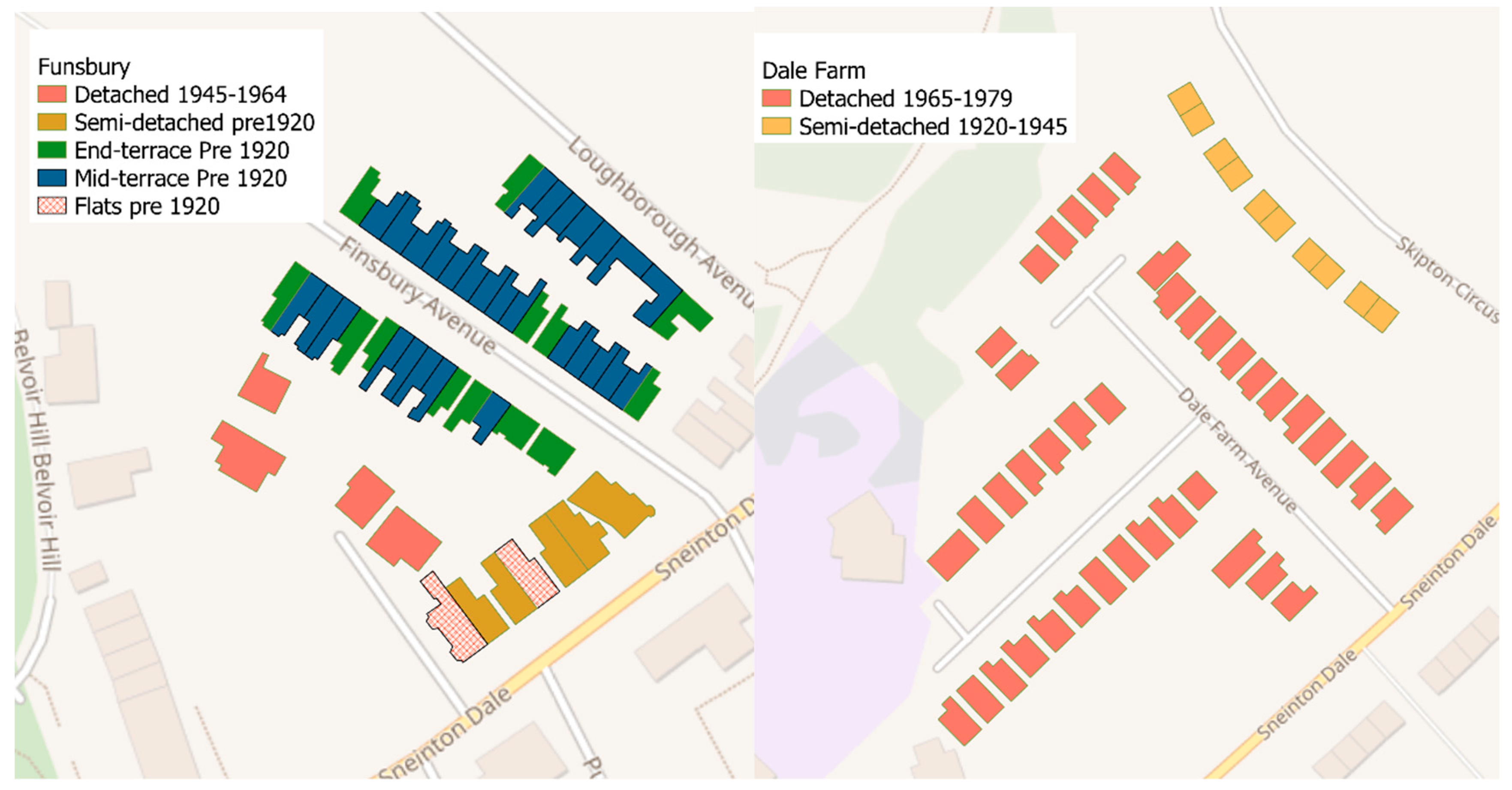
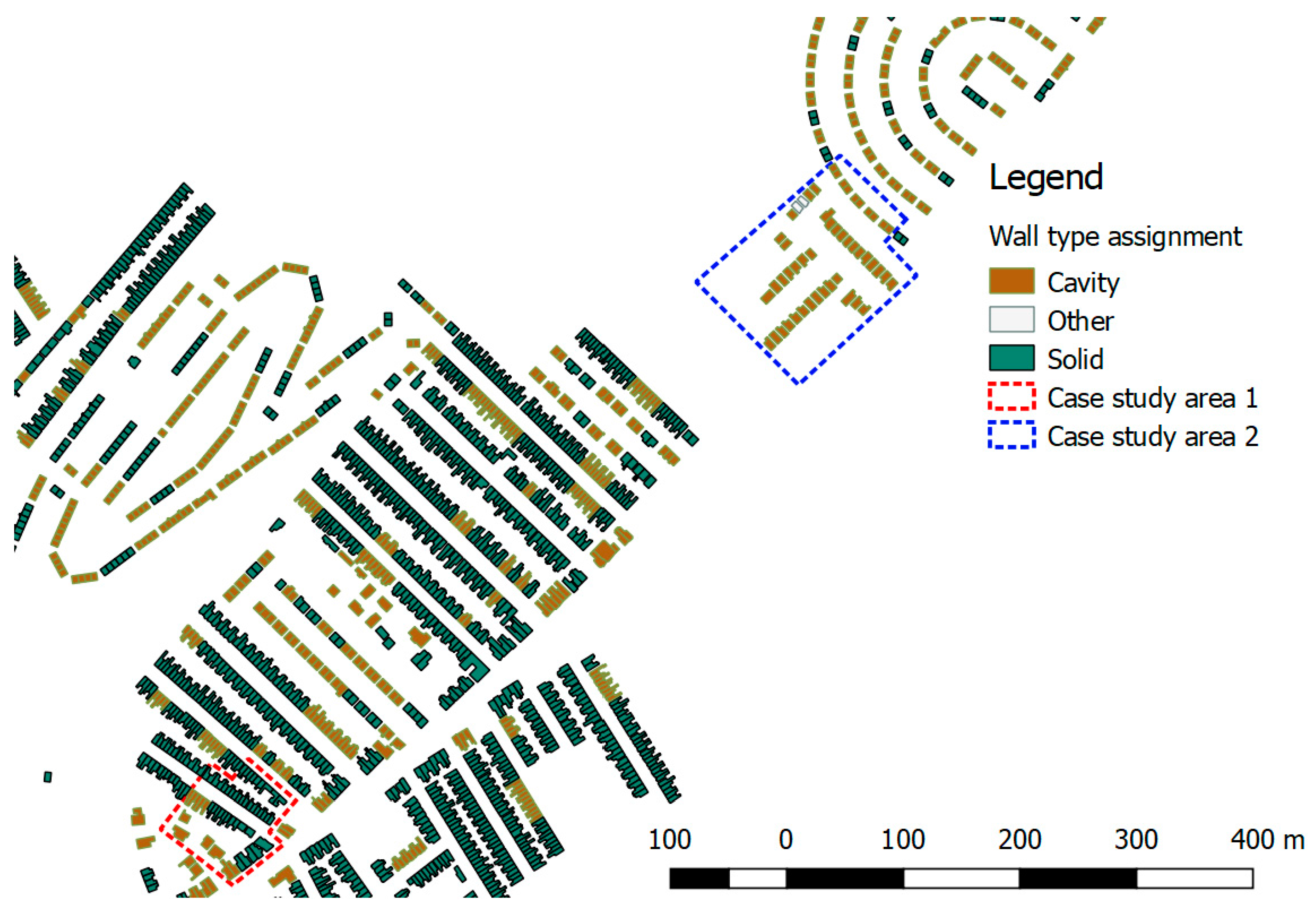
In order to speed up the execution of CitySim+, we have run all simulations over the University of Nottingham HPC. The CitySim+ code was enhanced to utilise high-performance OpenMP and was compiled for use with the software configuration available on the HPC nodes. OpenMP is a set of compiler instructions (or hints in C++ compiler terms) and function calls which enable sections of the CitySim+ code to run in parallel over a shared memory parallel computing node (for simplicity we call it a multicore node). It manages a set of threads that occupy the different cores on the multicore node, with each thread representing a small unit of work that can occupy the central processing unit (CPU) to complete a task assigned by the parent process.

As the scene size grows, computational resources, in terms of CPU time and memory, become a limiting factor. For example, a CitySim+ simulation consumes ~1.6 hours of total CPU time to simulate the hourly shortwave irradiance distribution over a scene comprised of ~800 buildings, or ~5000 surfaces, in the case of complex roof models over the whole year. The total CPU time accounts for all the time the simulation process requested the CPUs (i.e., it appends all the time consumed by individual threads in a multithreaded program like CitySim+). To accelerate our computations, we perform simulations using nodes with General Purpose Graphic Processing Unit (GPGPU) support (called Enhanced nodes). The typical specification for these nodes is listed in

Table 4. Hardware specification for General Purpose Graphic Processing Unit (GPGPU) node.

Variable	Value
No. of CPUs	2
CPUs model	Intel Sandybridge E5-2650 2.0 GHz
No. of cores	2 × 8
Total memory	32 GB
No. GPGPUs	2
GPGPU model	Nvidia M2090
Disk space	500 GB

.

3. Case Study Areas

Two case study areas (each containing approximately 50 residential buildings) were chosen to illustrate the workflow to create energy-attributed models for simulation. The case studies are both located within the Sneinton district of the city of Nottingham, each exhibiting very different building types. These two case study areas were selected as they represent a broad diversity of building age and form and include a range of residential building types that are common within the city of Nottingham. Maps showing the building footprints and layout for the case study areas are shown in Figure 5. The buildings in case study area 1 include some complex geometrical footprints and contrast with the simpler building footprints present in case study 2. The difference in geometric complexity provides an effective comparison of the impact of geometric simplification on simulation performance and accuracy. All the buildings in both case studies are residential dwellings.

Case study 1 (Finsbury) is a group of buildings built prior to 1915 and includes rows of two storey terraced buildings along with some larger 2- and 3-storey semidetached and detached buildings. These types of building are very common in the city (and the UK generally) and are usually constructed using solid masonry walls. A map showing the building footprints and layout for the case study area is shown in Figure 5.

Case study 2 (Dale Farm) has buildings of mixed vintage: detached private houses built in the 1970s and semidetached social housing built in the 1920s. All the buildings in Dale farm are two storeys.

In estimating the nonspatial attributes of the case study models, a number of assumptions were made:

• All buildings were heating to the required heating set-point temperature from 07:00 to 23:00 from 1st October until 1st May. A setback temperature of 5 °C was applied at all other times.
• No cooling system was specified.
• None of the buildings had a room present in the roof.
• Household composition and occupancy levels were fixed for all buildings at two adults, present at all times.

These assumptions were considered reasonable; recall the aim of this paper is not to simulate a realistic energy demand for the case studies, but to illustrate the described workflow and to examine the effects of geometric simplification on simulation performance and accuracy.

4. Results

Here we demonstrate application of our workflow for modelling urban scenes and its application for energy simulation for the two case study areas. Section 4.1 reports on the energy attribution modelling. Section 4.2 illustrates the estimates of building energy usage when employed for microsimulation, while Section 4.3 assesses the effect of geometric simplification on the computational and energy performance of the simulation.

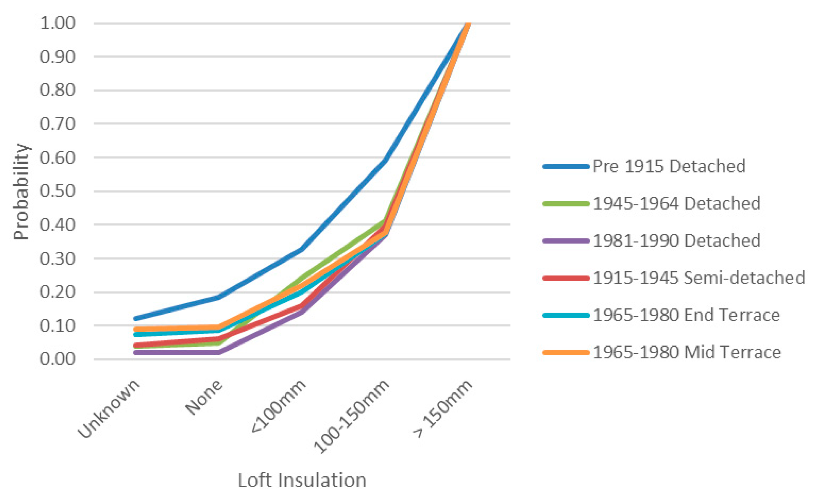
4.1. Statistical Model Energy Attribution Results

The attribution method described in Section 2.5 was used to populate the nonspatial energy parameters for the housing stock of the city of Nottingham (~100,000 properties). A comparison of the average statistics for the two case study areas and the city housing stock is shown in

Table 5. Statistics for energy parameter attribution for two case study areas and the city.

Parameter	Case Study 1	Case Study 2	Nottingham City
Average heating set-point temperature	20.3 °C	19.1 °C	20.5 °C
Average infiltration rate (ach)	0.73	0.74	0.67
Percentage of insulated walls	9%	52%	45%
Median loft insulation level	>150 mm	>150 mm	>150 mm
Percentage of double-glazed buildings	85%	94%	93%
Average thermal volume	292.5 m3	309.7 m3	335.9 m3

. Average values for case study 2 are similar to those for the city housing stock. In comparison, case study 1 has very few buildings with insulated walls, a higher number of single glazed buildings (15% vs. 7%) and smaller than average thermal volumes (i.e., the volume of the building that requires heating). As expected, from the central limit theorem, the average HSP for the city of Nottingham is 20.5 °C. Figure 6 illustrates spatially resolved examples of the parameter attribution. As described, wall types are assigned to blocks of buildings rather than the individual buildings within each block.

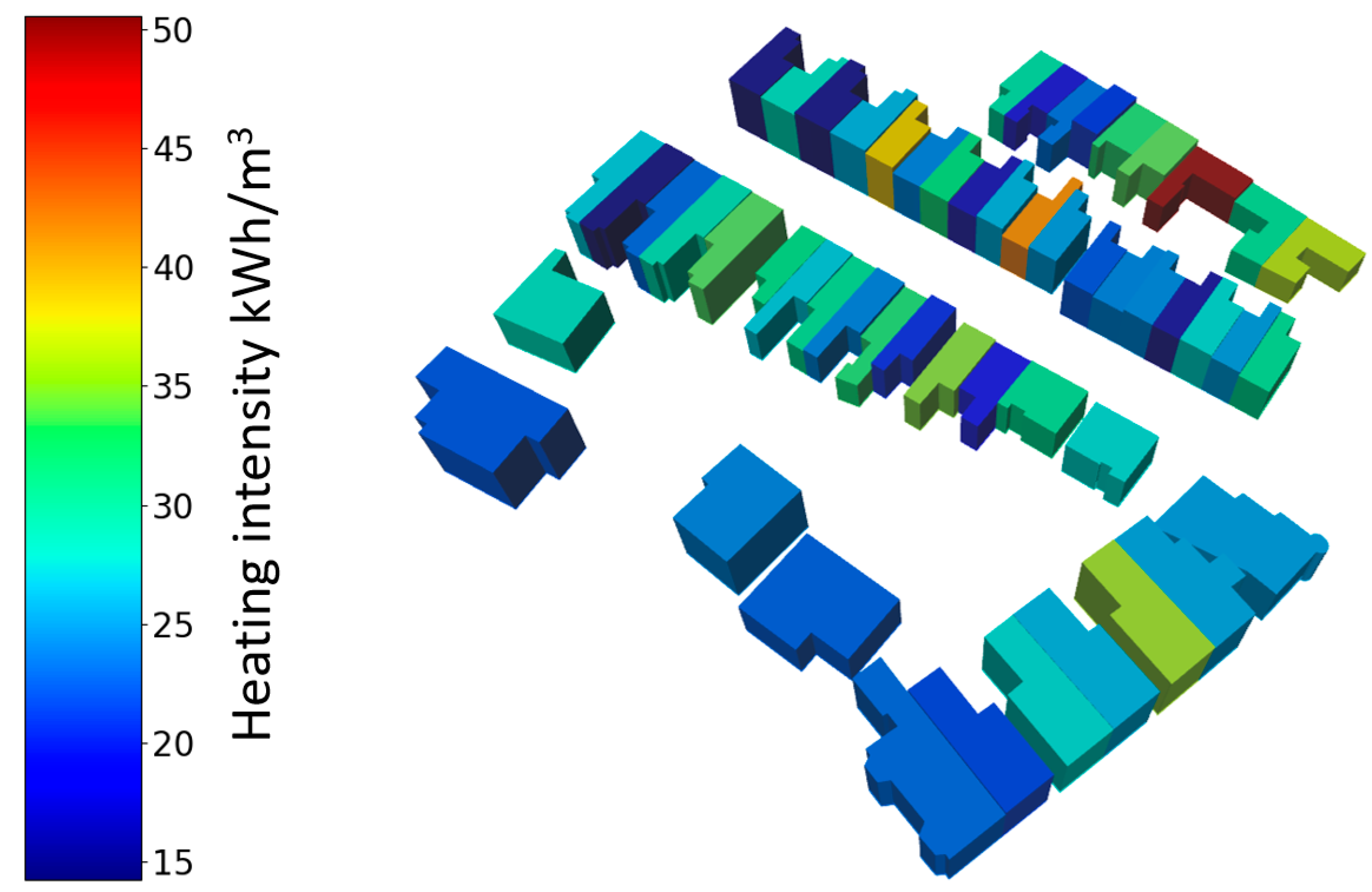
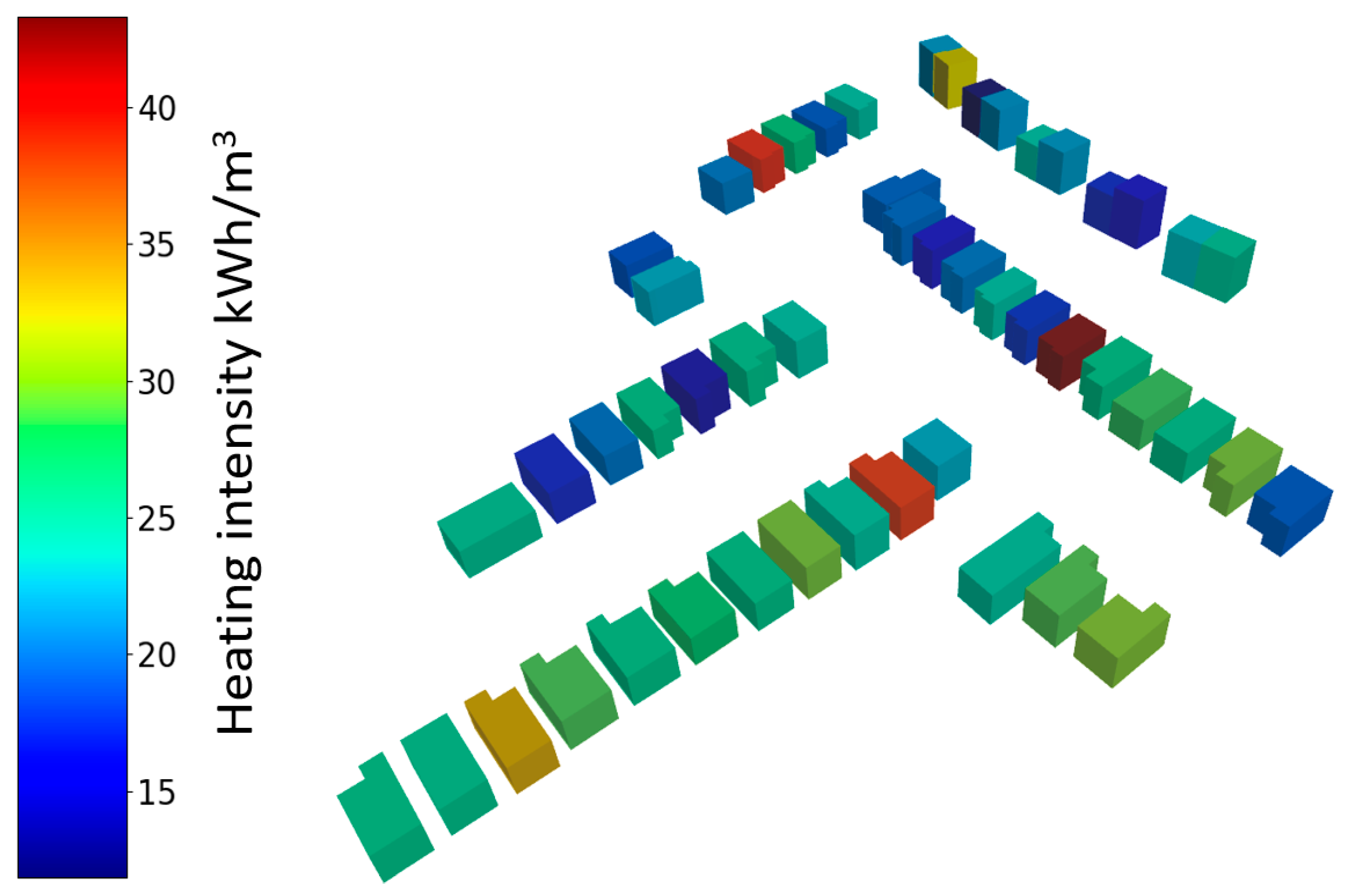
4.2. Energy Simulation Results

Running the simulations for each of the case study areas enables visualisation of the total annual heat demand for each building. We present the heat demand by volume, expressed as energy use intensity per m³. As expected, the older and more poorly insulated buildings in case study area 1 have higher heat demands (Figure 7) than those in case study area 2 (Figure 8). Average heat demand in case study 1 is 7.76 MWh and total heat demand is 411 MWh, compared to an average of 7.54 MWh and total of 377 MWh for case study 2. This is in line with the OFGEM Typical Domestic Consumption Value (TDCV) for a low-user (https://www.ofgem.gov.uk/gas/retail-market/monitoring-data-and-statistics/typical-domestic-consumption-values), when assuming that 85% of gas use is attributed to space heating [43]. The buildings in both areas that have the highest heat demands are typically uninsulated houses with higher heating set-points and infiltration rates.

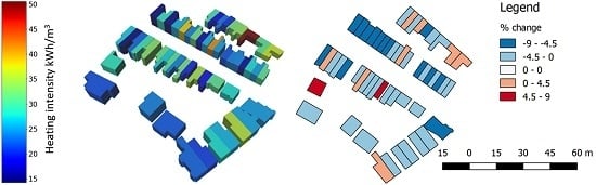
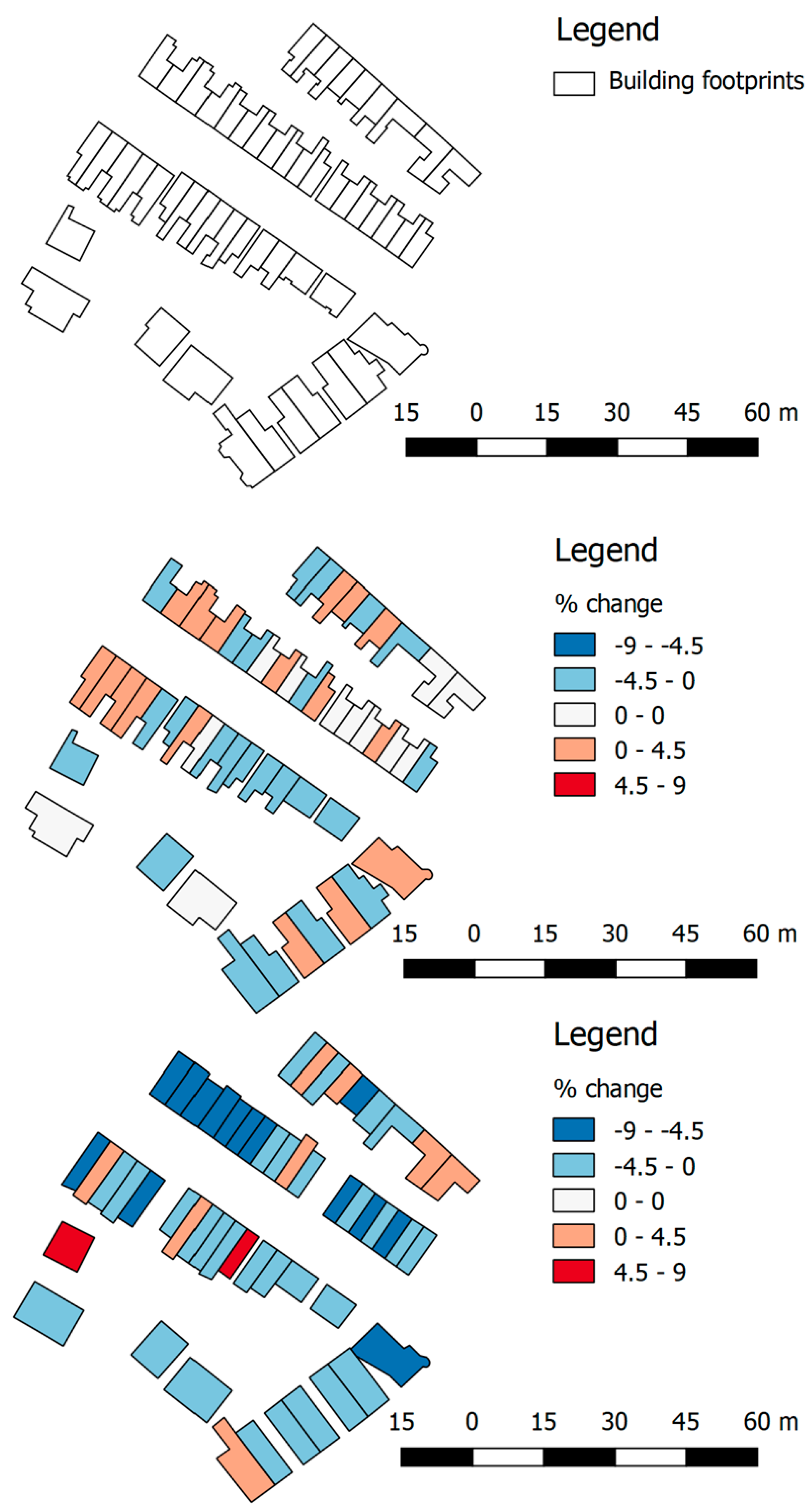
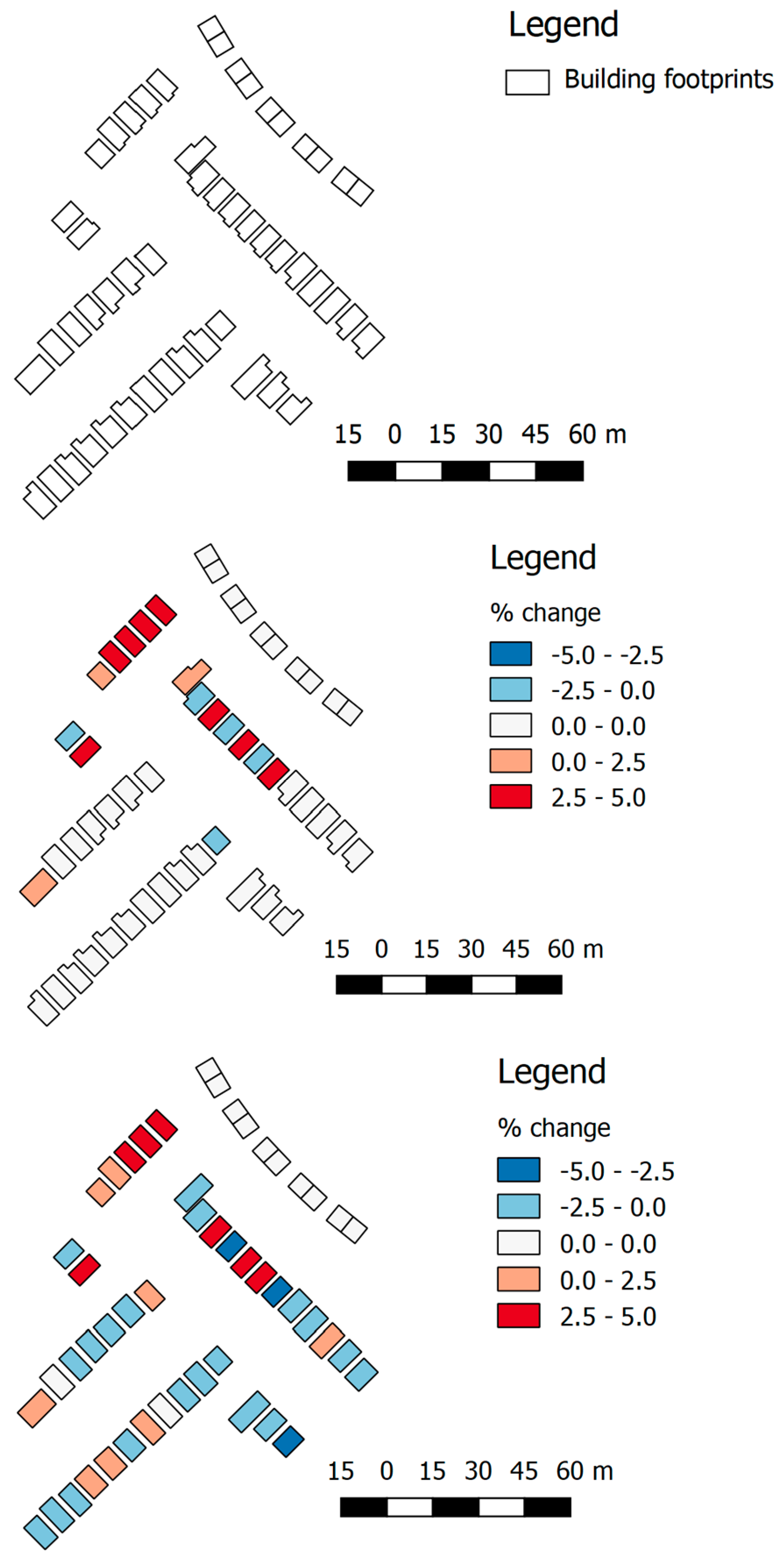
4.3. Building Simplification Results

Table 6. Building simplification results, reduction of vertices, surfaces, and the effect on heat demand for case study areas 1 and 2.

	Base Model	1 m Simplified	3 m Simplified
	Finsbury—Case Study Area 1
Number of 2D vertices	472	403	312
Number of ThermalBoundary surfaces	525	456	365
Reduction in surfaces (%)	n/a	13	30
Total heat demand (MWh)	411.32	411.06	402.84
Average heat demand (kWh)	7760.76	7755.86	7600.70
Heat demand difference (%)	n/a	−0.06	−2.00
Total Simulation seq. time (mins)	88.09	79.0	54.46
Simulation seq. time reduction (%)	n/a	10.31	38.17
	Dale Farm—Case Study Area 2
Number of 2D vertices	314	286	250
Number of ThermalBoundary surfaces	364	336	300
Reduction in surfaces (%)	n/a	8	18
Total heat demand (MWh)	377.18	379.60	376.08
Average heat demand (kWh)	7543.69	7591.97	7521.56
Heat demand difference (%)	n/a	+0.64	−0.29
Total Simulation seq. time (mins)	83	68	57.17
Simulation seq. time reduction (%)	n/a	18.39	31.22

illustrates the effect of building footprint generalisation on the resulting model complexity according to thresholds of 1 and 3 m. The reduction in the number of overall surfaces is the most important aspect in decreasing simulation time. Notably there is an obvious difference in the simplification between the two study areas, with case study area 1 exhibiting 5 and 12 higher percentage point reductions in the number of simulated surfaces than case study area 2, at the respective generalisation thresholds. This is due to the relatively simple building shapes found in case study area 2, of which a proportion are already rectangular and thus cannot be simplified further.

Table 6 also describes the overall change in heating demand from the base model at the different simplification levels, with Figure 9 and Figure 10 illustrating percentage change at the per-building level. At the 1-m-level, we see that the estimates remain relatively close to the baseline, for example in case study 2 the overall heat demand difference is within ~0.5%. At the 3-m-level, the geometry changes have a more notable effect. For example, considering the mid-terraces in Figure 9, the simplify algorithm tends to remove protruding parts the footprint that extend away from the main footprint shape leading to tighter packing of the footprints in the block—this appears to reduce the exposed wall area, decreasing the heating demand.

5. Discussion

We found that several assumptions were necessary in the development of this workflow and highlight several interesting avenues for further work. Our workflow is described for the UK context, where detailed footprint geometry, address and energy survey information is readily available to practitioners. However, the workflow would be applicable in other contexts (potentially with minor adaptation). For example, results from the simplification exercise in described this paper demonstrated that detailed footprint geometry is not necessarily required to produce reasonable energy estimates. Most EU countries would have data on housing stocks that could be used to populate the nonspatial energy parameters in EnergyADE (see for example the EU Building Stock Observatory). This could then be supplemented by data on local housing stock features where available.

One key finding relates to the lack of geometric generalisation algorithms appropriate to the energy modelling context, i.e., that maintain rectilinearity in the building shape, footprint area (and thus envelope volume) and topology (i.e., adjacency relations between buildings). As such, we adopt and evaluate the generalisation of the 2D building footprints using an off-the-shelf GIS package (ArcGIS), with automated postprocessing to resolve invalidation of the adjacency relations and thus maintain appropriate shared wall geometry and attribution in the energy model. This reduces the number of surfaces in the resulting model, greatly reducing the computational complexity of the scene and the corresponding cost, with a relatively modest degradation in the heating demand estimate (2% underestimation at most).

Applying a single generalisation threshold to urban scenes comprised of different building morphologies is a relatively crude approach. Investigation of the application of different thresholds according to built form or building archetype could be a valuable area for further work. There is likely an ideal threshold to apply at the footprint or block level. Going further, an ideal generalisation approach would aim to maintain exposed wall area (i.e., where heat loss is most drastic), footprint area or building volume, topology and tie-in knowledge of the wall construction (such as likelihood of cavity or solid wall presence). For example, negative effects of generalisation (deviations in the energy demand accuracy) are strongest when an external wall is uninsulated and these cases could be handled with less severe geometric changes.

In terms of EnergyADE modelling, the geometric volume defined for simulation in this work is a single zone; however, the EnergyADE standard supports composition of multiple geometric zones within a building envelope. This could form part of future work. Furthermore, EnergyADE attribution of nonspatial parameters can be performed using national or local surveys of housing stocks where applicable. Where such data is not available or is lacking in key attributes, default values can be applied based on expert knowledge. Housing archetypes can be used to assign attributes to the urban housing stock. In the UK, the EHS is a good source of attribution data due to the size of the survey sample and the frequency of update. It does, however, produce homogenous results and cannot capture local differences in building construction methods and/or design. This limitation could be overcome by using the recently available Energy Performance Certificate dataset, as an alternative or supplement to the EHS data [41]. Supplementing the results with other local data or expert knowledge can also be used to mitigate this limitation.

The use of a dynamic, spatially explicit energy simulation (CitySim+) to predict energy use offers a significant improvement over current approaches to energy modelling. In the UK context, energy performance of buildings is typically assessed using the BRE’s Standard Assessment Procedure (SAP) in its standard or reduced data (rdSAP) version [44]. This simplified model uses energy balance equations to predict residential energy use on a monthly or annual basis and does not provide the level of fidelity of a full dynamic energy simulation. See Kelly et al. [44] and Jenkins et al. [45] for a more detailed discussion of the limitations of SAP based energy predictions.

6. Conclusions

Efficiently creating urban housing stock models for energy simulation is a challenging task due to the range of information required to accurately represent the characteristics of each building in the scene, and the level of detail available in existing datasets. In addition, ensuring that such models can be consumed by different simulator applications and that computational complexity can be managed, particularly for larger urban scenes, are important requirements in solving this challenge. This article demonstrates a workflow for the creation of residential scenes encoded using CityGML and EnergyADE schemas. Taking national mapping agency data as the basis for the geometric information, we describe constructing the relevant surface and volume features using attributes of building height and extrusion of 2D footprints. For the energy related features, we statistically modelled residential building characteristics based on a national housing survey sample and used this model to infer likely per-building values for attributes defined by EnergyADE schema. To understand how the computational overhead associated with dynamic simulation could be reduced, we integrated an off-the-shelf geometric simplification routine as part of the workflow. Our experiments show that reducing the number of surfaces with a strong generalisation tolerance led to, at most, a small underestimation (2%) in heating demand with a 30% reduction in the number of simulated surfaces.

We have demonstrated the application of the workflow described in this paper for relatively small UK scenes. Work is underway to improve the ways in which these scenes can be handled, in conjunction with hardware acceleration technology, to facilitate larger, potentially city-scale, microsimulation.

References

1. BEIS. Energy Consumption in the UK (ECUK); 2017; Department for Business Energy and Industrial Strategy report. Available online: https://www.gov.uk/government/statistics/energy-consumption-in-the-uk (accessed on 1 December 2017).
2. Reinhart, C.F.; Davila, C.C. Urban building energy modeling: A review of a nascent field. Build. Environ. 2016, 97, 196–202. [Google Scholar] [CrossRef]
3. Cetin, K.; Wang, Y.; Chen, G.; Li, W.; Zhang, X.; Zhou, Y.; Eom, J. Modeling urban building energy use: A review of modeling approaches and procedures. Energy 2017, 141, 2445–2457. [Google Scholar]
4. Sousa, G.; Jones, B.M.; Mirzaei, P.A.; Robinson, D. A review and critique of UK housing stock energy models, modelling approaches and data sources. Energy Build. 2017, 151, 66–80. [Google Scholar] [CrossRef]
5. Kavgic, M.; Mavrogianni, A.; Mumovic, D.; Summerfield, A.; Stevanovic, Z.; Djurovic-Petrovic, M. A review of bottom-up building stock models for energy consumption in the residential sector. Build. Environ. 2010, 45, 1683–1697. [Google Scholar] [CrossRef]
6. Davila, C.C.; Reinhart, C.; Bemis, J. Modeling Boston: A workflow for the generation of complete urban building energy demand models from existing urban geospatial datasets. Energy 2016, 117, 237–250. [Google Scholar] [CrossRef]
7. Nouvel, R.; Zirak, M.; Coors, V.; Eicker, U. The influence of data quality on urban heating demand modeling using 3D city models. Comput. Environ. Urban Syst. 2017, 64, 68–80. [Google Scholar] [CrossRef]
8. Chen, Y.; Hong, T.; Luo, X.; Hooper, B. Development of city buildings dataset for urban building energy modeling. Energy Build. 2019, 183, 252–265. [Google Scholar] [CrossRef]
9. Julia, S.; Davila, C.; Reinhart, R.C. Validation of a Bayesian-based method for defining residential archetypes in urban building energy models. Energy Build. 2017, 134, 11–24. [Google Scholar]
10. Robinson, D.; Haldi, F.; Kämpf, J.H.; Leroux, P.; Perez, D.; Rasheed, A.; Wilke, U. CITYSIM: Comprehensive Micro-Simulation of Resource Flows for Sustainable Urban Planning. In Proceedings of the Eleventh International IBPSA Conference, Glasgow, UK, 27–30 July 2009; pp. 1083–1090. [Google Scholar]
11. Wilke, U.; Haldi, F.; Scartezzini, J.; Robinson, D. A bottom-up stochastic model to predict building occupants’ time-dependent activities. Build. Environ. 2013, 60, 254–264. [Google Scholar] [CrossRef]
12. Fuchs, M.; Teichmann, J.; Lauster, M.; Remmen, P.; Streblow, R.; Müller, D. Workflow automation for combined modeling of buildings and district energy systems. Energy 2016, 117, 478–484. [Google Scholar] [CrossRef]
13. Kaden, R.; Kolbe, T.H. Simulation-Based Total Energy Demand Estimation of Buildings using Semantic 3D City Models. Int. J. 3D Inf. Model. 2014, 3, 35–53. [Google Scholar] [CrossRef]
14. Frayssinet, L.; Merlier, L.; Kuznik, F.; Hubert, J.; Milliez, M. Modeling the heating and cooling energy demand of urban buildings at city scale. Renew. Sustain. Energy Rev. 2018, 81, 2318–2327. [Google Scholar] [CrossRef]
15. Robinson, D.; Stone, A. Solar radiation modelling in the urban context. Sol. Energy 2004, 77, 295–309. [Google Scholar] [CrossRef]
16. Keirstead, J.; Jennings, M.; Sivakumar, A. A review of urban energy system models: Approaches, challenges and opportunities. Renew. Sustain. Energy Rev. 2012, 16, 3847–3866. [Google Scholar] [CrossRef]
17. Groger, G.; Plumer, L. CityGML—Interoperable semantic 3D city models. ISPRS J. Photogramm. Remote Sens. 2012, 71, 12–33. [Google Scholar] [CrossRef]
18. Wate, P.; Coors, V. 3D data models for urban energy simulation. Energy Procedia 2015, 78, 3372–3377. [Google Scholar] [CrossRef]
19. Wieland, M.; Wendel, J. Computing Solar Radiation on CityGML Building Data. In Proceedings of the 18th AGILE International Conference on Geographic Information Science, Lisbon, Portugal, 9–12 June 2015; pp. 2–5. [Google Scholar]
20. Giovannini, L.; Pezzi, S.; di Staso, U.; Prandi, F.; de Amicis, R. Large-Scale Assessment and Visualization of the Energy Performance of Buildings with Ecomaps—Project SUNSHINE: Smart Urban Services for Higher Energy Efficiency. In Proceedings of the 3rd International Conference on Data Management Technologies and Applications, Vienna, Austria, 29–31 August 2014; pp. 170–177. [Google Scholar]
21. Paiho, S.; Ketomäki, J.; Kannari, L.; Häkkinen, T.; Shemeikka, J. A new procedure for assessing the energy-efficient refurbishment of buildings on district scale. Sustain. Cities Soc. 2019, 46, 101454. [Google Scholar] [CrossRef]
22. Kaden, R.; Kolbe, T. City-wide total energy demand estimation of buildings using semantic 3D city models and statistical data. In Proceedings of the ISPRS Annals of the Photogrammetry, Remote Sensing and Spatial Information Sciences, ISPRS 8th 3DGeoInfo Conference & WG II/2 Workshop, Istanbul, Turkey, 27–29 November 2013; Volume II-2/W1. [Google Scholar]
23. Murshed, S.M.; Koch, A. Modelling, Validation and Quantification of Climate and Other Sensitivities of Building Energy Model on 3D City Models. ISPRS Int. J. Geo-Inf. 2018, 7, 447. [Google Scholar] [CrossRef]
24. Agugiaro, G.; Benner, J.; Cipriano, P.; Nouvel, R. The Energy Application Domain Extension for CityGML: Enhancing interoperability for urban energy simulations. Open Geospat. Data Softw. Stand. 2018, 3, 2. [Google Scholar] [CrossRef]
25. Wagner, D.; Wewetzer, M.; Bogdahn, J.; Alam, N. Geometric-Semantical Consistency Validation of CityGML Models. In Progress and New Trends in 3D Geoinformation Sciences; Springer: Berlin/Heidelberg, Germany, 2013; pp. 171–192. [Google Scholar]
26. Zhao, J.; Ledoux, H.; Stoter, J.; Feng, T. ISPRS Journal of Photogrammetry and Remote Sensing HSW: Heuristic Shrink-wrapping for automatically repairing solid-based CityGML LOD2 building models. ISPRS J. Photogramm. Remote Sens. 2018, 146, 289–304. [Google Scholar] [CrossRef]
27. Gröger, G.; Kolbe, T.H.; Nagel, C.; Häfele, K. OpenGIS City Geography Markup Language (CityGML) Encoding Standard; Version 2.0.0, OGC Doc. No. 12-019; Open Geospatial Consortium: Wayland, MA, USA, 2012. [Google Scholar]
28. Beck, A.; Long, G.; Boyd, D.S.; Rosser, J.F.; Morley, J.; Duffield, R.; Sanderson, M.; Robinson, D. Automated classification metrics for energy modelling of residential buildings in the UK with open algorithms. Environ. Plan. B Urban Anal. City Sci. 2018. [Google Scholar] [CrossRef]
29. Wate, P.; Coors, V.; Iglesias, M.; Robinson, D. Uncertainty assessment of building performance simulation: An insight into suitability of methods and their applications. In Urban Energy Systems for Low-Carbon Cities; Eicker, U., Ed.; Academic Press: Cambridge, MA, USA, 2019; pp. 257–287. ISBN 978-0-12-811553-4. [Google Scholar]
30. Long, G.; Alwany, M.; Robinson, D. Building Typologies Simulation Report, Nottingham. Available online: http://www.insmartenergy.com/wp-content/uploads/2014/12/D.2.1.-Simulation_Report_for_building_Typologies-Nottingham.pdf (accessed on 12 July 2017).
31. Energy Saving Trust. CE54: Domestic Heating Sizing Method. 2010. Available online: https://www.energysavingtrust.org.uk/policy-research/ce54-domestic-heating-sizing-method-2011 (accessed on 3 March 2017).
32. Firth, S.K.; Lomas, K.J.; Wright, A.J. Targeting household energy-efficiency measures using sensitivity analysis. Build. Res. Inf. 2010, 38, 24–41. [Google Scholar] [CrossRef]
33. Gasden, S.J.; Rylatt, R.M.; Lomas, K.J. Methods of predicting urban domestic energy demand with reduced datasets: A review and a new GIS-based approach. Build. Serv. Eng. Res. Technol. 2003, 24, 93–102. [Google Scholar]
34. Aksoezen, M.; Daniel, M.; Hassler, U.; Kohler, N. Building age as an indicator for energy consumption. Energy Build. 2015, 87, 74–86. [Google Scholar] [CrossRef]
35. Rosser, J.F.; Boyd, D.S.; Long, G.; Zakhary, S.; Mao, Y.; Robinson, D. Predicting residential building age from map data. Comput. Environ. Urban Syst. 2019, 73, 56–67. [Google Scholar] [CrossRef]
36. DCLG. English Housing Survey: Technical Report, 2014–2015. 2015. Available online: https://assets.publishing.service.gov.uk/government/uploads/system/uploads/attachment_data/file/552532/2014-15_EHS_Technical_Report_-_all_chapters_and_annexes.pdf (accessed on 3 March 2017).
37. Jones, B.; Das, P.; Chalabi, Z.; Davies, M.; Hamilton, I.; Lowe, R.; Mavrogianni, A.; Robinson, D.; Taylor, J. Assessing uncertainty in housing stock infiltration rates and associated heat loss: English and UK case studies. Build. Environ. 2015, 92, 644–656. [Google Scholar] [CrossRef]
38. BRE. Energy Follow-Up Survey 2011. Report 2: Mean Household Temperatures. 2013. Available online: https://assets.publishing.service.gov.uk/government/uploads/system/uploads/attachment_data/file/274770/2_Mean_Household_Temperatures.pdf (accessed on 3 March 2017).
39. Kane, T.; Firth, S.K.; Lomas, K.J. How are UK homes heated? A city-wide, socio-technical survey and implications for energy modelling. Energy Build. 2015, 86, 817–832. [Google Scholar] [CrossRef]
40. Huebner, G.M.; McMichael, M.; Shipworth, D.; Shipworth, M.; Durand-Daubin, M.; Summerfield, A. Heating patterns in English homes: Comparing results from a national survey against common model assumptions. Build. Environ. 2013, 70, 298–305. [Google Scholar] [CrossRef]
41. Stephen, R. Airtightness in UK Dwellings; IHS BRE Press: Watford, UK, 2000. [Google Scholar]
42. Robinson, D.; Campbell, N.; Gaiser, W.; Kabel, K.; Le-Mouel, A.; Morel, N.; Page, J.; Stankovic, S.; Stone, A. SUNtool—A new modelling paradigm for simulating and optimising urban sustainability. Sol. Energy 2007, 81, 1196–1211. [Google Scholar] [CrossRef]
43. Department of Energy & Climate Change Estimates of Heat Use in the United Kingdom in 2013. Available online: https://assets.publishing.service.gov.uk/government/uploads/system/uploads/attachment_data/file/386858/Estimates_of_heat_use.pdf (accessed on 1 February 2018).
44. Kelly, S.; Crawford-Brown, D.; Pollitt, M.G. Building performance evaluation and certification in the UK: Is SAP fit for purpose? Renew. Sustain. Energy Rev. 2012, 16, 6861–6878. [Google Scholar] [CrossRef]
45. Jenkins, D.; Simpson, S.; Peacock, A. Investigating the consistency and quality of EPC ratings and assessments. Energy 2017, 138, 480–489. [Google Scholar] [CrossRef]
Figure 1. Overview of the proposed workflow. The outline of the process “Footprint simplification” is dashed as it is an optional procedure.
Ijgi 08 00163 g001
Figure 2. Our Cumulative Distribution Functions (CDFs) of glazing types for example archetypes.
Ijgi 08 00163 g002
Figure 3. Our Cumulative Distribution Functions (CDFs) of loft insulation for example archetypes.
Ijgi 08 00163 g003
Figure 4. Energy ADE, UML and XML representation for a solid masonry wall.
Ijgi 08 00163 g004
Figure 5. Case study area (Finsbury) 1 (left) and case study area (Dale Farm) 2 (right).
Ijgi 08 00163 g005
Figure 6. Wall type assignment for the Sneinton area of Nottingham with case study areas highlighted.
Ijgi 08 00163 g006
Figure 7. Heat demand by volume (CitySim+ thermal model) results for case study 1.
Ijgi 08 00163 g007
Figure 8. Heat demand by volume (CitySim+ thermal model) results for case study 2.
Ijgi 08 00163 g008
Figure 9. Case study area 1: Raw unsimplified footprints (top) and percentage change in heat demand between base model and 1 m simplification (middle) and 3 m simplification (bottom).
Ijgi 08 00163 g009
Figure 10. Case study area 2: Raw unsimplified footprints (top) and percentage change in heat demand between base model and 1 m simplification (middle) and 3 m simplification (bottom).
Ijgi 08 00163 g010