Multi-Constrained Optimization Method of Line Segment Extraction Based on Multi-Scale Image Space

Abstract

Image-based line segment extraction plays an important role in a wide range of applications. Traditional line segment extraction algorithms focus on the accuracy and efficiency, without considering the integrity. Serious line segmentation fracture problems caused by image quality will result in poor subsequent applications. To solve this problem, a multi-constrained line segment extraction method, based on multi-scale image space, is presented. Firstly, using Gaussian down-sampling with a classical line segment detection method, a multi-scale image space is constructed to extract line segments in each image scale and all line segments are projected onto the original image. Then, a new line segment optimization and purification strategy is proposed with the horizontal and vertical distances and angle geometric constraint relationships between line segments to merge fracture line segments and delete redundant line segments. Finally, line segments with adjacent positions are optimized using the grayscale constraint relationship, based on normalized cross-correlation similarity criterion for realizing the second optimization of fracture line segments. Compared with mainstream line segment detector and edge drawing lines methods, experimental results (i.e., indoor, outdoor, and aerial images) indicate the validity and superiority of our proposed methods which can extract longer and more complete line segments.

1. Introduction

The line feature is an important part of an image’s geometric information and plays a crucial role in photogrammetry and remote sensing [1], three-dimensional (3D) urban modeling [2,3], computer vision and robot navigation positioning [4,5], and so on. Simultaneously, the importance of line elements is emphasized in cartography and the even more user-oriented discipline, spatial cognition [6,7]. The line feature has the following advantages as a more advanced feature than the point feature: (1) It has rich structural information for expressing edge information of 3D objects, such as structured buildings; (2) the extraction of the line feature is less affected by image noise, occlusion, geometric distortion, and grayscale distortion; (3) it has higher matching accuracy; (4) it is not necessary to completely determine the position of its two endpoints; and (5) in case of missing texture or uniformity, the line feature is easier to extract than the point feature. Particularly, a line feature is the kind of rich structural information which can intuitively express edge contours of the structured scene. This has achieved good practical application results in scientific and engineering decision-making applications. Crowley [8] and Zhang et al. [9] used line features to realize map creation and navigation positioning. Garulli et al. [10] utilized lines to express environmental features, enabling simultaneous localization and mapping (SLAM) of mobile robots for sensing unknown environments. Trinh et al. [11] extracted line segments from the surface of structured buildings to achieve a shape analysis of the target. Yu et al. [12] detected the location of cracks in pipes by judging whether the line feature was continuous. Elqursh et al. [13] proposed a bundle-adjustment method combined with line segments to achieve relative orientation of stereo-images and the estimated position and pose information of the camera. Gerke [14] and Schmude [15] used line segments as the constraint information for a camera’s relative orientation. Santos et al. [16] combined the line feature extraction algorithm to implement unmanned aerial vehicle (UAV) image-based power line inspections. Partovi [17] extracted straight lines from a building feature and used them for the regularized processing of buildings. Wang et al. [18] used reconstructed 3D line segments as auxiliary information to improve the quality of the real orthophoto that reduced the sawtooth pull problem at the edge of a building. Therefore, it is valuable to extract good line features in many fields.

Line segment extraction algorithms can be classified into three categories: (1) Algorithms that transform domain-based methods [19]; (2) algorithms based on gradient phase feature [20]; and (3) segmentation edge approaches [21]. The first type of algorithm is less influenced by image noise, but the calculation cost is higher, with lower extraction accuracy. The second type of algorithm has a low memory-occupancy rate with better extraction efficiency in complex scenes, but it is sensitive to grayscale distortion. When the grouping error is large, line segments are prone to the phenomenon of obvious segmentation fracture. The third type of method can detect local features of the image and it is easy to obtain the geometric attribute information of the line segment. Its extraction speed is fast, yet these algorithms depend on the quality of built-in edge tracking algorithms.

The theoretical basis of line segment extraction is relatively mature. The Hough transform technique [22] extracts line segments accurately in a single texture background scene, but it is prone to large error-extracted line segments in complex texture scenes. Xu et al. [23] proposed a multi-scale Hough transform with a pre-stored weight matrix to detect straight lines with higher precision and less constraints by studying the limitation of accuracy, efficiency, and image size for detecting line segments of Hough transform. Canny [24] proposed the line segment extraction algorithm with edge detection based on the Canny operator. However, the algorithm requires a large number of decision-making parameters, which has serious false positive (false detection) and false negative (missing detection) problems. A robust line segment extraction algorithm progressive probabilistic Hough transform (PPHT) proposed by Matas et al. [25] combines the random edge point selection algorithm to improve the feature extraction speed. However, its error-detection mechanism easily raises false negatives and misses the necessary short line segments. More recently, a local line segment extraction algorithm, line segment detector (LSD), proposed by Gioi et al. [26], was found to be capable of extracting sub-pixel-level precision line segments in linear time, but the effect of line segments intersection, partial occlusion, image blur, image noise, and grayscale distortion caused severe segmentation fracture problems. Akinlar et al. [27,28] proposed a new edge detection operator, Edge Drawing, and a faster line segment extraction algorithm, Edge Drawing Lines (EDLines), but the segmentation fracture effect of the extracted line segments was not improved. The false negative of this method is inevitable and it is easy to miss critical line segments.

The existing research mainly focuses on the accuracy and efficiency of the line feature extraction without considering the length of extracted line segments. Short line segments are less accurate than long line segments, which causes more processing errors (error matching and error reconstruction). Currently, there are few methods to solve this line segmentation fracture problem. To alleviate this common problem, this paper proposes a multi-constrained line segment extraction optimization algorithm based on multi-scale image space, namely MSLines, including MSLSD and MSEDLines (MS is an abbreviation of Multi-Scale), which reduces the influence of grayscale distortion on feature extraction using the idea of fuzzy processing.

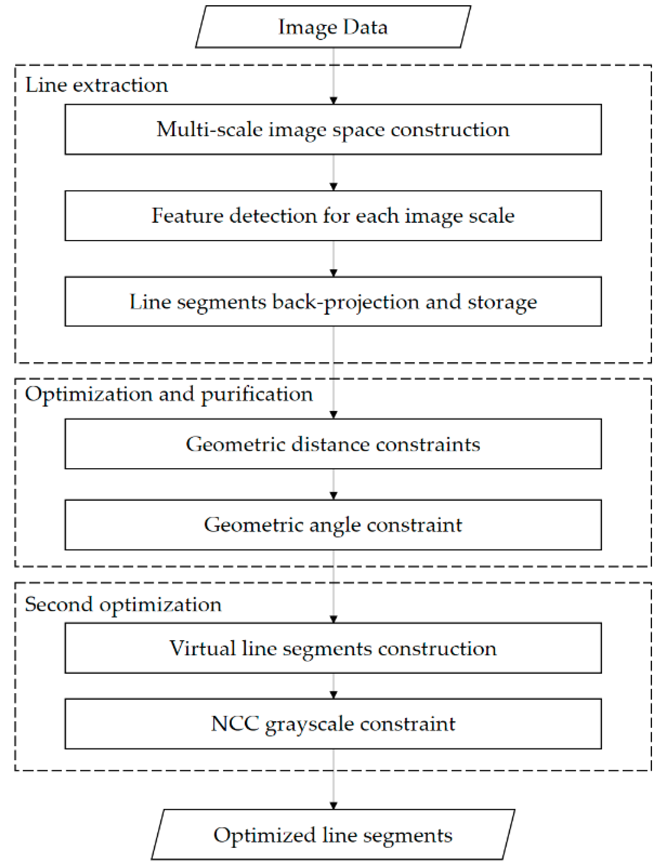
Figure 1 shows the overall methodology presented in this paper, which is divided into three main modules. The first module consists of constructing the line segment extraction model. A multi-scale image pyramid was constructed based on the Gaussian down-sampling and line segments of each image layer were extracted by the traditional line segment detection algorithm. All line segments were projected onto the original image and stored in line vector spaces. The second module was the optimization of the purification strategy. A set of line segment optimization and purification methods were designed with geometric constraints; line segments were merged or deleted according to the distance and angle relationships between line segments. The third module was second optimization. The virtual straight line was constructed and the secondary merge optimization of the line segment was realized based on the grayscale constraint relationship of the normalized cross correlation (NCC) measurement. Compared with several mainstream line segment extraction algorithms, i.e., LSD and EDLines, the proposed method could alleviate the segmental fracture effect of line segments and eliminate line segments’ redundant problem.

The remainder of this study is organized as follows. Section 2 describes the principle of multi-scale image space line segment extraction method. This section also introduces a new line segment optimization and purification method based on geometric constraints. Also, a second optimization method of grayscale constraint is presented. In Section 3, three sets of real data, i.e., indoor, outdoor, and aerial images are tested to analyze superiority of our proposed line segment extraction method compared with the mainstream method. Section 4 discusses the selection of parameters in the model construction for various resolution images and analyses the accuracy of the proposed method. Section 5 presents conclusions and possible further studies.

2. Methods

2.1. Model Construction

2.1.1. Line Segment Detection Method

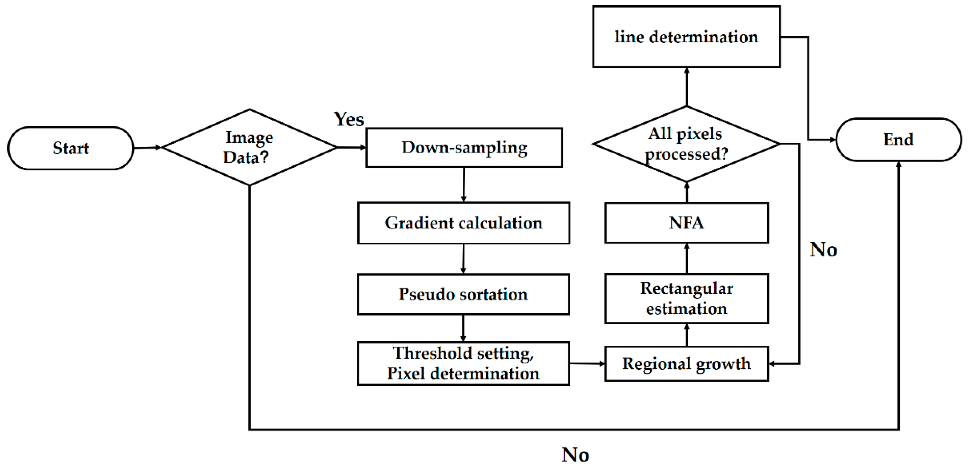
At present, Von Gioi’s LSD line segment extraction algorithm is one of the most widely used methods. The principle of several mainstream line segment extraction algorithms is similar to LSD. Figure 2 shows the workflow of the LSD algorithm.

In the line detection process, the input image was first down-sampled to 80% of the original image by the Gaussian down-sampling method to weaken the sawtooth effect of image, as well as to maintain a balance between the sawtooth effect and image blur. Next, a 2 × 2 gradient template was given to calculate the gradient direction (level-line angle (LLA)) and amplitude (intensity) of all pixels after image down-sampling. Depending on the pixel gradient amplitude, 1024 containers were opened and all image pixels were pseudo sorted from high to low order. Simultaneously, a state list was established and the initial state of all pixels was set to UNUSED. The state of pixel labels whose gradient amplitude was smaller than the threshold “ρ” was changed to USED, to represent an area where the image is flat or the gradient changes slowly; this means it did not participate in the line support region (LSR) and rectangle construction. Then, an UNUSED pixel from the sorted list was selected as a seed point. The region growing algorithm was used to generate LSR with the seed point. The seed point and LLA were continuously updated until the current point could not meet the threshold requirement. The final regional direction angle θ_reg was achieved. The rectangle and the number of false alarms (NFA) was calculated according to θ_reg and finally, line segments were determined after traversing all UNUSED seed points.

A point can only belong to certain line segment with a traditional LSD algorithm where extracted line segments cannot intersect with each other. If two line segments intersect, they break and split into four short line segments. Additionally, the algorithm is susceptible to pixel grayscale gradient mutation during the regional growth period, so that the difference between the current point LLA and the regional direction angle exceeds the growth threshold, resulting in segmentation fracture of the line segments. The EDLines algorithm uses the Edge Drawing operator for feature extraction. The speed of this method is fast, but the line segmentation fracture problem is not improved. Therefore, traditional line segment extraction algorithms should be further optimized to solve the segmentation fracture effect.

2.1.2. Multi-Scale Image Space Line Segment Extraction Method

In order to overcome the segmentation fracture problem of line segment extraction, the proposed method combines the idea of fuzzy processing by down-sampling the original image to produce a pyramid-like model of multi-scale image space.

To perform this method, the specific procedure was as follows: (1) According to the actual image resolution and processing requirements, the standard deviation factor (scale space factor) of Gaussian filter kernel function σ was set and the maximum down-sampling number t_max was set; (2) Gaussian kernel convolution on image I to achieve Gaussian blur of the image was performed; (3) image-based down-sample on image-scale space factor σ (σ is generally set to 0.5) was carried out; (4) to detect line segment, the traditional method was used for this layered image and the line segments were stored in the corresponding line vector spaces; (5) steps (2 –4) were repeated until the maximum number of down-sampling was reached. Specifically, the Gaussian-blurred image $I^{\prime }\left(u,v,\sigma \right)$ is first generated with Equation (1).

$$\{\begin{array}{c}{I}^{\prime }\left(u,v,\sigma \right)=G\left(u,v,\sigma \right)\ast I\left(u,v\right)\\ G\left(u,v,\sigma \right)=1/2\pi {\sigma }^2\ast \exp \left(-(u^2+v^2)/2{\sigma }^2\right)\end{array},$$

(1)

where $G\left(u,v,\sigma \right)$ is the Gaussian kernel function, $I\left(u,v\right)$ is the image $I$, and $*$ is the convolution operation on the image pixel $\left(u,v\right)$.

Based on scale space factor σ, the original image was down-sampled to obtain a low-resolution image J. The above operation was repeated to continue down-sampling of image J until the maximum down-sampling number t_max was reached. Finally, an N-layer image model was created (N = t_max + 1), forming a pyramid-like multi-scale image space model.

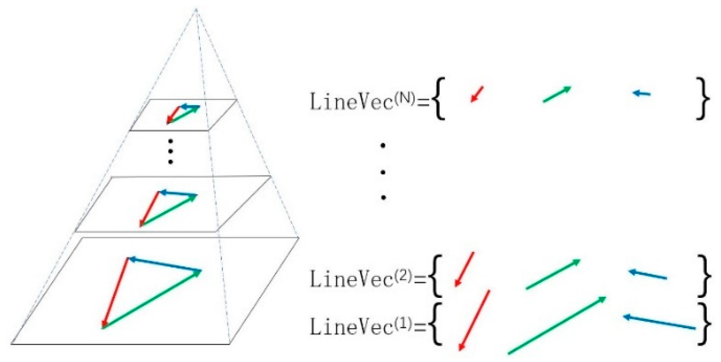
To detect line segments, traditional line segment detection method was used for each image layer in scale space and line segment vector spaces corresponding to the number of images were opened. Line segments extracted in each scale image were stored in a line segment vector $LineVe{c}^{(k)}=\left\{\right\}$, where k represents the k-scale image of line segment vector space and the maximum value of k is N. Moreover, line segment endpoints’ coordinates and length information were stored in line segment class $lin{e}_i^{\left(k\right)}=\left\{u_{start}^{\left(i\right)},v_{start}^{\left(i\right)},u_{end}^{\left(i\right)},v_{end}^{\left(i\right)},lengt{h}^{\left(i\right)}\right\}$, where ^k represents kth line segment vector space and ⁱ represents ith line in the image. Line segment extraction and storage process is shown in Figure 3.

Figure 3 shows that the traditional line segment detector extracts line segments for each scale image and stores segments in vector space. If detector extracts m₁ and m₂ line segments in the first and second layers of the image, respectively, then the line segment method extracts m_N line segments in the Nth layer of the image. The expression of multi-scale image space line feature vector can be represented with Equation (2).

$$\{\begin{array}{c}LineVe{c}^{\left(1\right)}=\left\{lin{e}_1^{\left(1\right)},lin{e}_2^{\left(1\right)},lin{e}_3^{\left(1\right)},\cdots ,lin{e}_{m_1}^{\left(1\right)}\right\}\\ LineVe{c}^{\left(2\right)}=\left\{lin{e}_1^{\left(2\right)},lin{e}_2^{\left(2\right)},lin{e}_3^{\left(2\right)},\cdots ,lin{e}_{m_2}^{\left(2\right)}\right\}\\ ⋮\\ LineVe{c}^{\left(N\right)}=\left\{lin{e}_1^{\left(N\right)},lin{e}_2^{\left(N\right)},lin{e}_3^{\left(N\right)},\cdots ,lin{e}_{m_N}^{\left(N\right)}\right\}\end{array}$$

(2)

2.1.3. Line Segment Projection

Line segments extracted from different scale images were all projected to the original image and stored in a new opened memory vector space. Particularly, line segments extracted from the original image were directly stored in a new vector. For a line segment extracted after down-sampling of image, the $lin{e}_i^{{\left(k\right)}^{*}}$ needed to be projected with Equation (3) in case of known scaling factor σ and the number of the image down-sampled times t ($t=k-1$). Finally, a vector set SumLineVec of all line segments extracted by traditional method in the multi-scale image space was achieved with Equation (4). The vector dimension of SumLineVec is m₁ + m₂ + ⋯ + m_N.

$$lin{e}_i^{{\left(k\right)}^{*}}={\left(\frac{1}{\sigma }\right)}^{k-1}\times \left\{u_{start}^{\left(i\right)},v_{start}^{\left(i\right)},u_{end}^{\left(i\right)},v_{end}^{\left(i\right)},lengt{h}^{\left(i\right)}\right\},$$

(3)

$$SumLineVec=\left\{LineVe{c}^{{\left(N\right)}^{*}},LineVe{c}^{{\left(N-1\right)}^{*}},\cdots ,LineVe{c}^{{\left(1\right)}^{*}}\right\},$$

(4)

where,

$$\{\begin{array}{c}LineVe{c}^{{\left(1\right)}^{*}}=\left\{lin{e}_1^{{\left(1\right)}^{*}},lin{e}_2^{{\left(1\right)}^{*}},lin{e}_3^{{\left(1\right)}^{*}},\cdots ,lin{e}_{m_1}^{{\left(1\right)}^{*}}\right\}\\ LineVe{c}^{{\left(2\right)}^{*}}=\left\{lin{e}_1^{{\left(2\right)}^{*}},lin{e}_2^{{\left(2\right)}^{*}},lin{e}_3^{{\left(2\right)}^{*}},\cdots ,lin{e}_{m_2}^{{\left(2\right)}^{*}}\right\}\\ ⋮\\ LineVe{c}^{{\left(N\right)}^{*}}=\left\{lin{e}_1^{{\left(N\right)}^{*}},lin{e}_2^{{\left(N\right)}^{*}},lin{e}_3^{{\left(N\right)}^{*}},\cdots ,lin{e}_{m_N}^{{\left(N\right)}^{*}}\right\}\end{array}.$$

(5)

2.2. Optimization and Purification Based on Geometric Constraints

After line segments extracted by the multi-scale image space were projected to the original image, severe redundancy. Overlapping. and clutter problems of line segments occur. Many line segments are meaningless, so the entire set of line segments needs to be optimized and purified. As a result, the down-sampled image with low resolution can only extract a few segments, which brings extraction error. In this subsection, a line segment optimization and purification strategy is proposed, which optimizes line segment extraction results through line segment geometric constraint relationships. The optimized line segments have longer length and higher integrity, while alleviating the redundancy problem.

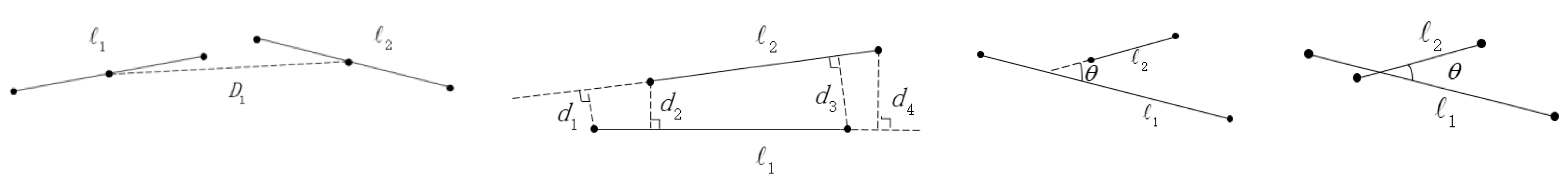
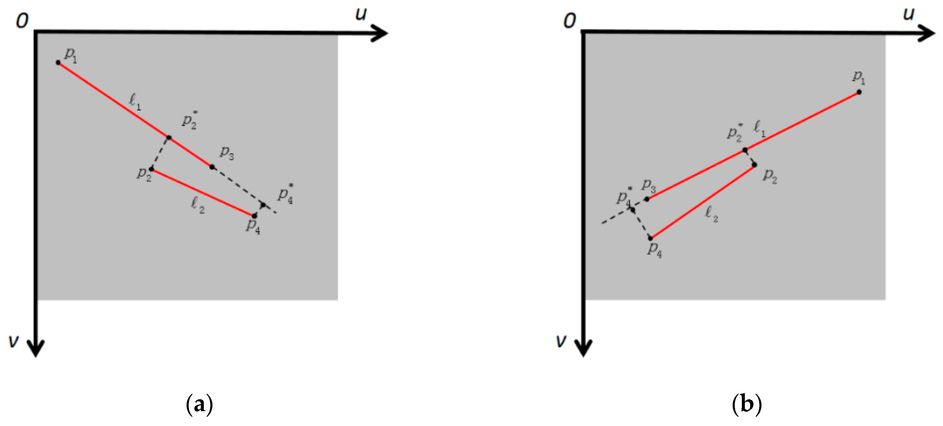
Before optimization and purification, it is necessary to describe and determine constraint relationships between line segments. As shown in Figure 4, the geometric constraint relationships between line segments are defined as follows:

Based on the geometric constraint relationships in Figure 4, we define horizontal, vertical, and angle thresholds to determine whether line segments need to be optimized and purified. We define $l_1=\left\{u_1^{\left(1\right)},v_1^{\left(1\right)},u_2^{\left(1\right)},v_2^{\left(1\right)},lengt{h}^{\left(1\right)}\right\}$ and $l_2=\left\{u_1^{\left(2\right)},v_1^{\left(2\right)},u_2^{\left(2\right)},v_2^{\left(2\right)},lengt{h}^{\left(2\right)}\right\}$, respectively, as reference and determined line segments that needed to be judged. The distance between midpoints of two segments is $D_1=\frac{1}{2}\sqrt{{\left(u_1^{\left(1\right)}+u_2^{\left(1\right)}-u_1^{\left(2\right)}-u_2^{\left(2\right)}\right)}^2+{\left(v_1^{\left(1\right)}+v_2^{\left(1\right)}-v_1^{\left(2\right)}-v_2^{\left(2\right)}\right)}^2}$ and the average distance between the endpoints of two segments is $D_2=\left(d_1+d_2+d_3+d_4\right)/4$. The angle between two lines is θ.

2.2.1. Distance Geometric Constraint

The distance geometric constraint relationships can be divided into horizontal and vertical distance relationships. Considering the horizontal distance relationship (Figure 4a), the distance D₁ between the midpoints of two line segments is used to judge whether they are related and whether $l_2$ needs to be retained or deleted. If $D_1>\left(lengt{h}^{\left(1\right)}+lengt{h}^{\left(2\right)}\right)/2$, $l_2$ and $l_1$ are independent. $l_2$ is retained and stored as one of the reference line segments in the next judgment process. If $D_1\le \left(lengt{h}^{\left(1\right)}+lengt{h}^{\left(2\right)}\right)/2$, $l_2$ is related to $l_1$ and $l_2$ continues to be judged by the vertical distance constraint relationship. Considering vertical distance constraint (Figure 4b), if $D_2\le {\xi }_d$ (where ${\xi }_d$ is the vertical threshold), $l_2$ is strongly correlated with $l_1$ and we then merge $l_1$ and $l_2$. If ${\xi }_d<D_2\le 3{\xi }_d$, $l_2$ is a redundant or invalid segment and needs to be deleted. If $D_2>3{\xi }_d$, $l_2$ and $l_1$ are independent and $l_2$ is retained and stored as one of the reference line segments in the next judgment. Here we set ξ_d = 1(pixel), because the resolution of the human eye is 1 pixel, and the error of more than 1 pixel is discernible.

In this paper, as a part, we also propose an optimization method for merging short line segments based on endpoint projection transformation. The reason for selecting optimization method is that the least squares fitting method has larger extraction errors for extracted line segments from low-resolution images than from original images by using the multi-scale image space model. The least squares fitting is an error-averaging method to minimize the sum of squared errors. If the least squares fitting strategy was used here to merge line segments, it would bring more merging errors. The line segment merging method based on endpoint projection transformation is shown in Figure 5.

The origin O of an image coordinate system is located in the upper left corner of image. $l_1$ was a reference line segment extracted from the original image and the two endpoints were $p_1=\left(u_1,v_1\right)$ and $p_3=\left(u_3,v_3\right)$. $l_2$ was an error-containing line segment in the multi-scale image space and its two endpoints were $p_2=\left(u_2,v_2\right)$ and $p_4=\left(u_4,v_4\right)$, whereas $\widehat{p}=\left(u,v,1\right)$ were homogeneous coordinates corresponding to these endpoints. We projected error-containing line segments onto the reference line segment, as well as obtained projected coordinate values $p_2^{\ast }=\left(u_2^{\ast },v_2^{\ast }\right)$ and $p_4^{\ast }=\left(u_4^{\ast },v_4^{\ast }\right)$ at both endpoints of the error-containing line segment. Equation (6) gives the endpoint projection formula:

$$p^{\ast T}=\frac{1}{A^2+B^2}\left[\begin{array}{ccc}{B}^2& -AB& -AC\\ -AB& A^2& -BC\end{array}\right]{\widehat{p}}^T,$$

(6)

where A, B, and C are the reference line equation $Au+Bv+C=0$ parameters, which can be taken by known two endpoints image coordinates. Thereby, the projected coordinate value $p^{\ast }=\left(u^{\ast },v^{\ast }\right)$ of endpoints for the error-containing line segment can be achieved. Due to difference between positive and negative slopes of the reference line segment, the method of line segment merging has two possibilities regarding endpoint transformations. We can finally get endpoints $p_{first}=\left(u_{first},v_{first}\right)$ and $p_{last}=\left(u_{last},v_{last}\right)$ of the merged line segment using Equation (7).

$$\{\begin{array}{l}\begin{array}{cc}\begin{array}{l}\left(u_{first},v_{first}\right)=\left(\min \left\{u_1,u_2^{*},u_3,u_4^{*}\right\},\min \left\{v_1,v_2^{*},v_3,v_4^{*}\right\}\right)\\ \left(u_{last},v_{last}\right)=\left(\max \left\{u_1,u_2^{*},u_3,u_4^{*}\right\},\max \left\{v_1,v_2^{*},v_3,v_4^{*}\right\}\right)\end{array}& kRatio>0\end{array}\\ \begin{array}{cc}\begin{array}{l}\left(u_{first},v_{first}\right)=\left(\min \left\{u_1,u_2^{*},u_3,u_4^{*}\right\},\max \left\{v_1,v_2^{*},v_3,v_4^{*}\right\}\right)\\ \left(u_{last},v_{last}\right)=\left(\max \left\{u_1,u_2^{*},u_3,u_4^{*}\right\},\min \left\{v_1,v_2^{*},v_3,v_4^{*}\right\}\right)\end{array}& kRatio\le 0\end{array}\end{array}$$

(7)

2.2.2. Angle Geometric Constraint

When $l_2$ and $l_1$ intersect each other at the extension line (Figure 4c), there is no overlap between $l_1$ and $l_2$ due to that line segments are not infinitely long lines. Moreover, $l_1$ and $l_2$ don’t need to be judged by the angle geometric constraint relationship, but only the vertical distance geometric relationship is used for judgment. When $l_2$ intersects with $l_1$ at the non-extended line (Figure 4d), the angle constraint relationship is also judged for the deletion of the pseudo-line after completing the distance constraint judgment. If $\theta <{\xi }_{\theta }$ (where ${\xi }_{\theta }$ is the angle threshold, ξ_θ = 5°), we think that $l_2$ is a false line and delete it. Otherwise, we retain $l_2$. The expression of angle $\theta$ is given in Equation (8).

$$\theta =\left|\arctan \left(\left(v_2^{\left(2\right)}-v_1^{\left(2\right)}\right)/\left(u_2^{\left(2\right)}-u_1^{\left(2\right)}\right)\right)-\arctan \left(\left(v_2^{\left(1\right)}-v_1^{\left(1\right)}\right)/\left(u_2^{\left(1\right)}-u_1^{\left(1\right)}\right)\right)\right|$$

(8)

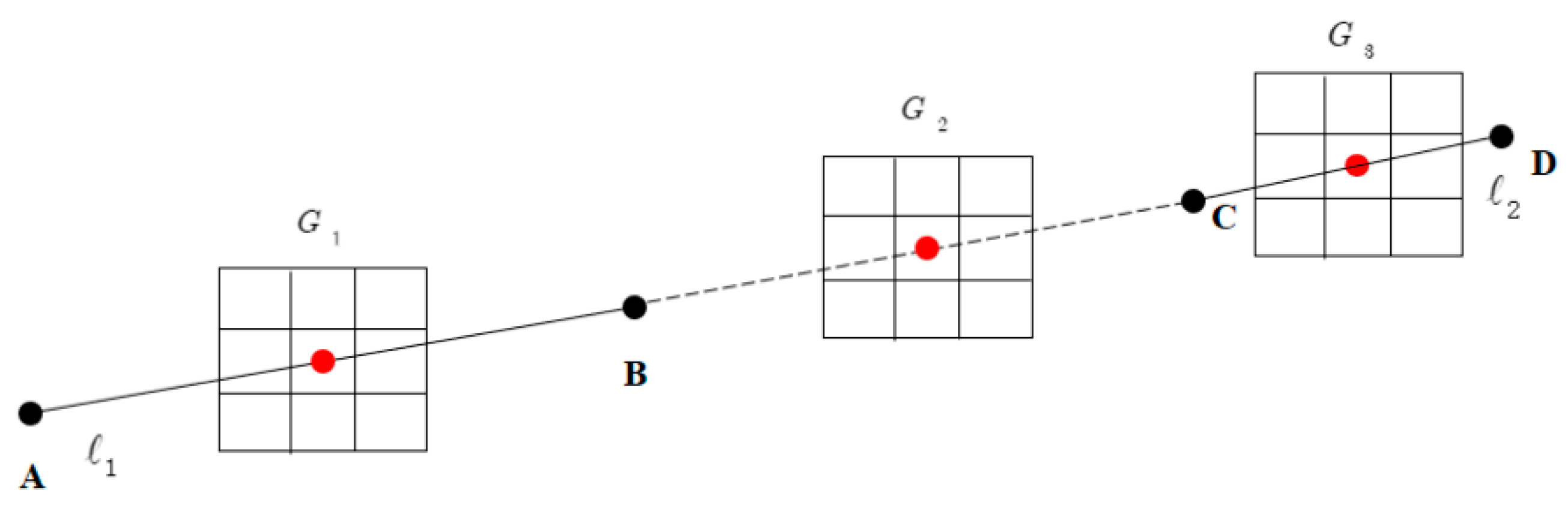
2.3. Optimization Based on Grayscale Constraint

After completing the geometric constraint relationship judgment, we can get optimized line segments. Grayscale constraint was performed on the first optimized line segment to realize the second optimization (Figure 6).

Furthermore, it must be mentioned that direction information of all line segments is traverse after geometric optimization. When any two line segments, $l_1$ and $l_2$, have the same direction (the angle between the two lines θ < 1°) and the distance between them is less than 20 pixels, which is suitable for the current typical megapixel/medium-resolution image in the experiment section of paper, these two line segments are temporarily merged into one virtual line segment.

In addition to this, grayscale points on the central positions of AB (midpoint of $l_1$), BC, and CD segments (midpoint of $l_2$) on virtual line segments are used as center grayscale to open a 3 × 3 matching window with NCC similarity judgment. NCC is often used to compare the similarity of two images and realize the matching features. Here, we propose an extended NCC that compares the similarities of the three windows (small patches) opened on one image. If $NCC\ge \psi$ (where $\psi$ is grayscale threshold among three matching windows, ψ = 0.8), the line segment has high grayscale-level similarity that means a virtual line segment is an optimized line segment. In this case, we combine $l_1$ and $l_2$ to get a real line segment. If $NCC<\psi$, the virtual line segment is not a real merging line segment. In this case, $l_1$ and $l_2$ are retained and the virtual line segment is released. The specific expression of NCC is given in Equation (9).

$$NCC=\frac{{\displaystyle \sum _{i,j=0}^{N-1}\left(G_p\left(i,j\right)-\frac{1}{N^2}{\displaystyle \sum _{i,j=0}^{N-1}{G}_p\left(i,j\right)}\right)\left(G_q\left(i,j\right)-\frac{1}{N^2}{\displaystyle \sum _{i,j=0}^{N-1}{G}_q\left(i,j\right)}\right)}}{\sqrt{{\displaystyle \sum _{i,j=0}^{N-1}{\left(G_p\left(i,j\right)-\frac{1}{N^2}{\displaystyle \sum _{i,j=0}^{N-1}{G}_p\left(i,j\right)}\right)}^2{\displaystyle \sum _{i,j=0}^{N-1}{\left(G_q\left(i,j\right)-\frac{1}{N^2}{\displaystyle \sum _{i,j=0}^{N-1}{G}_q\left(i,j\right)}\right)}^2}}}}\{\begin{array}{cc}p=1& q=2,3\\ p=2& q=3\end{array},$$

(9)

where G_p and G_q represent grayscale windows at positiond p and q on virtual line segment, respectively, and N represents the size of the grayscale window, which is 3 here.

2.4. Overall Procedure of Optimization

When the kth line segment in the SumLineVec line feature set was processed (k < dim), the previous k-1 line segments were used as reference lines for judgment. In this article, vertical distance constraint, angle constraint, and grayscale constraint thresholds were set respectively by the empirical method decision above.

According to the constraint relationships between line segments as described above, the specific procedure of line segment optimization and purification was as follows:

(1) The line feature vector space $R^1$ and $R^2$ were opened for storing line segments that were optimized by geometric and grayscale constraints. The initial state was $R^1=\left\{\right\}$ and $R^2=\left\{\right\}$.

(2) Line segments extracted from the original image in SumLineVec were taken as reference lines and directly taken into the optimized set $R^1$.

(3) Line segments extracted from other scale image space in SumLineVec were judged as determined lines with reference lines in the optimized set based on the geometric distance and angle constraint relationships. If the determined line satisfied the optimization and purification situation, $R^1$ would be updated. Otherwise, the determined line would be deleted.

(4) When all lines in SumLineVec were processed, an optimized set $R^1$ of line segments was obtained.

(5) For any two lines in $R^1$, virtual line segments were constructed by directional characteristics, where the grayscale constraint relationship was used for judgement. If two lines satisfied the grayscale constraint optimization situation, $R^2$ was optimized. Otherwise, those lines that do not need to be optimized were directly stored to $R^2$.

(6) The optimization set $R^2$ was purified by geometric constraint as a purification criterion. When geometric distance between line segments satisfies the culling condition, it was considered that there was a redundant line segment and we deleted the error. Also, when the angle distance between lines satisfied the culling condition, it was considered that there was a pseudo-line, which we deleted. Finally, we achieved the resulted line segment feature set $R^{2^{*}}$.

3. Experiments and Analysis

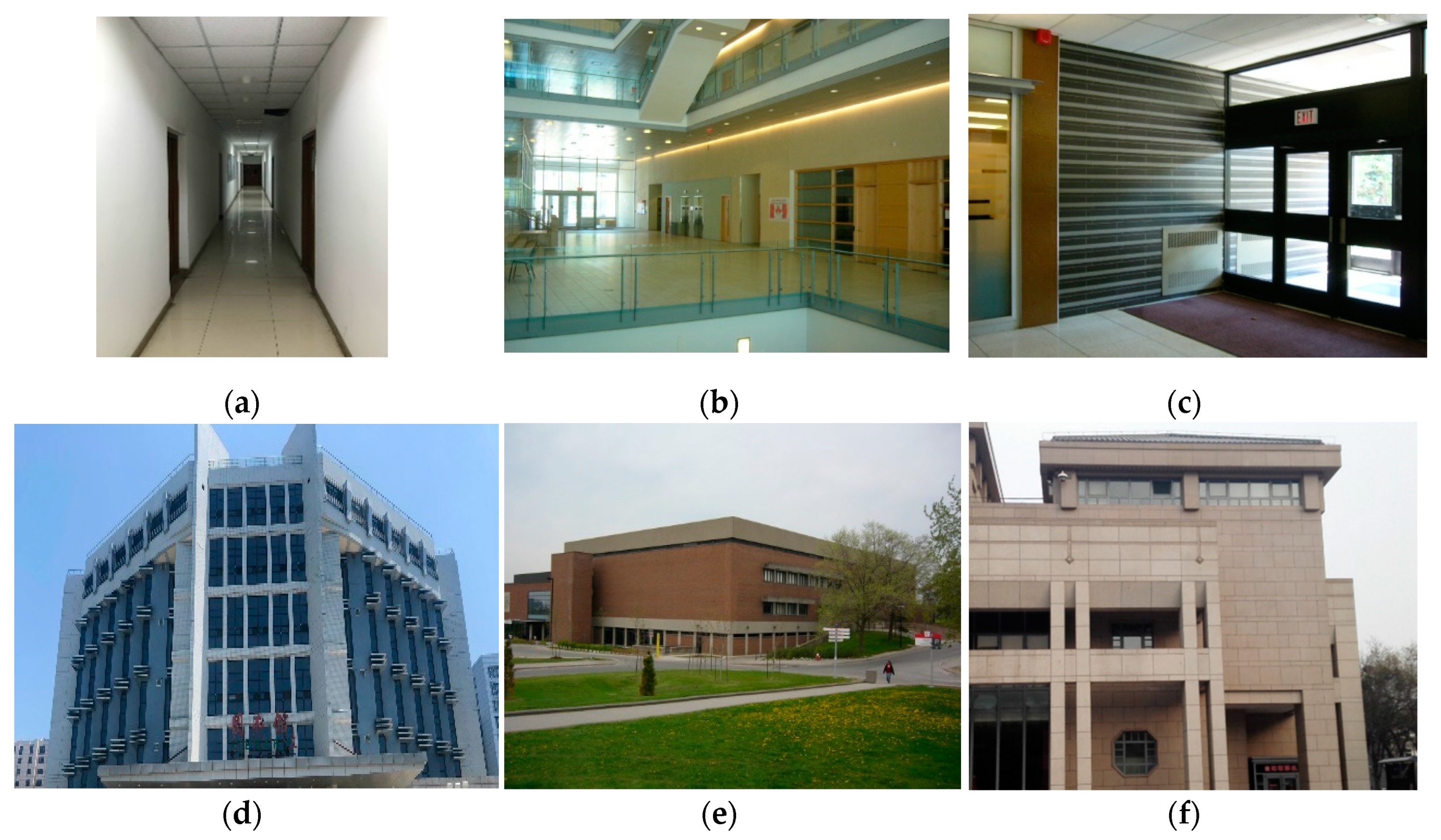
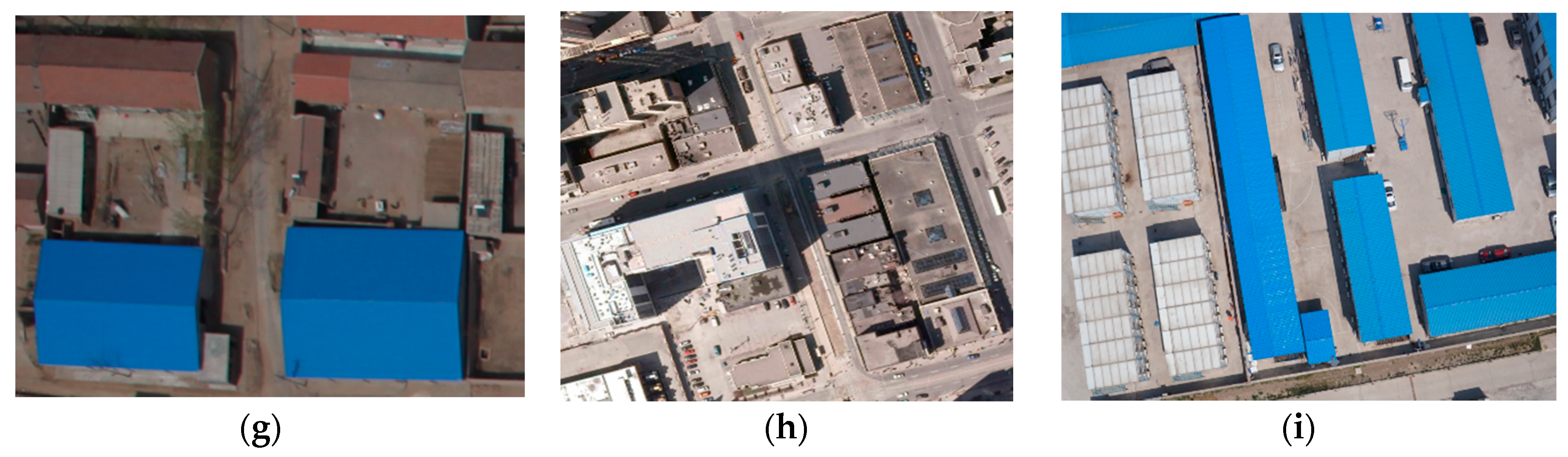
Experiments were carried out using three data sets, each with three images, i.e., indoor, outdoor, and aerial images, to verify the effectiveness of the proposed method, as shown in Figure 7. Our method was implemented in C++ and OpenCV. It was executed on a personal computer with Intel (R) Core (TM) i7-7500U 2.70 GHz CPU and 8.0 GB RAM.

As for the nine selected megapixel resolution data sets, we set the maximum down-sampling number t_max = 2 and scale space factor σ = 0.5 based on the parameter setting of discussion section. Therefore, a three-layered multi-scale image space model was formed. For the three sets of nine images, each image consists of three images with different resolutions arranged from high to low. Moreover, the merits of the proposed line segment extraction method (referred to as MSLSD and MSEDLines for better description) are mainly discussed from the aspect of number of extracted line segments, extraction time, accuracy rate, total length, average length, and visualization effect of the line segment extraction. Here, the accuracy rate is the ratio of the number of correctly extracted line segments to the total number of line feature extraction [29]. Generally, a longer average length of a line segment indicates a higher integrity of the extracted line, whereas a shorter extraction time means the method is better. However, this paper firstly uses the traditional method to extract line segments for multiple image scales and, as a result, extraction time is generally longer than the original method. The proposed method needs a short optimization time, but the overall extraction speed is not greatly affected. This study mainly solves the segmentation fracture problem of line segments and redundant or invalid feature problems. Therefore, it mainly focuses on the average and total lengths of line segments and the visualization effect of extracted line segments on the image. The proposed method is compared with LSD and EDLines methods from the above perspectives in this section.

For these test data, the line segment extraction results in Figure 8, Figure 9, Figure 10, Figure 11, Figure 12, Figure 13, Figure 14, Figure 15 and Figure 16 are, respectively, shown for conventional LSD, EDLines, and our proposed method, MSLSD, MSEDLines. Moreover, a quantitative index of traditional and proposed methods for line segment extraction in three sets of nine images is presented in

Table 1. Results of line segment extraction for indoor, outdoor, and aerial images using traditional and proposed methods.

Data	Methods	The Number of line Segments	Accuracy Rate	Time-consuming (s)	Total Length (pixel)	Average Length (pixel)
Indoor 1	EDLines	327	0.801	0.150	20633.7	63.1
	MSEDLines	215	0.842	0.359	18339.5	85.3
	LSD	445	0.879	0.586	22828.5	51.3
	MSLSD	238	0.874	0.636	20301.4	85.2
Indoor 2	EDLines	415	0.945	0.112	15977.5	38.5
	MSEDLines	276	0.960	0.122	14076.0	51.0
	LSD	463	0.944	0.214	16436.5	35.5
	MSLSD	303	0.967	0.269	13180.5	43.5
Indoor 3	EDLines	375	0.939	0.110	22950.0	61.2
	MSEDLines	253	0.960	0.133	18747.3	74.1
	LSD	487	0.959	0.221	26005.8	53.4
	MSLSD	299	0.963	0.272	21258.9	71.1
Outdoor 1	EDLines	1854	0.944	0.476	64890.0	35.0
	MSEDLines	1147	0.969	0.711	53450.2	46.6
	LSD	2196	0.954	1.425	70930.8	32.3
	MSLSD	1274	0.973	1.452	57584.8	45.2
Outdoor 2	EDLines	245	0.898	0.072	9016.0	36.8
	MSEDLines	158	0.810	0.084	8200.2	51.9
	LSD	265	0.894	0.237	8904.0	33.6
	MSLSD	162	0.907	0.273	7387.2	45.6
Outdoor 3	EDLines	631	0.973	0.200	25997.2	41.2
	MSEDLines	436	0.975	0.249	22192.4	50.9
	LSD	836	0.982	0.376	31099.2	37.2
	MSLSD	510	0.982	0.456	24939.0	48.9
Aerial 1	EDLines	395	0.975	0.112	12758.5	32.3
	MSEDLines	293	0.983	0.342	13448.7	45.9
	LSD	456	0.985	0.294	14044.8	30.8
	MSLSD	332	0.988	0.334	14342.4	43.2
Aerial 2	EDLines	901	0.964	0.230	33607.3	37.3
	MSEDLines	580	0.988	0.330	29580.0	51.0
	LSD	1064	0.963	0.785	31920.0	30.0
	MSLSD	642	0.989	1.142	26193.6	40.8
Aerial 3	EDLines	1126	0.947	0.546	34568.2	30.7
	MSEDLines	749	0.952	0.698	29735.3	39.7
	LSD	1313	0.950	0.753	33481.5	25.5
	MSLSD	875	0.966	1.029	29487.5	33.7

.

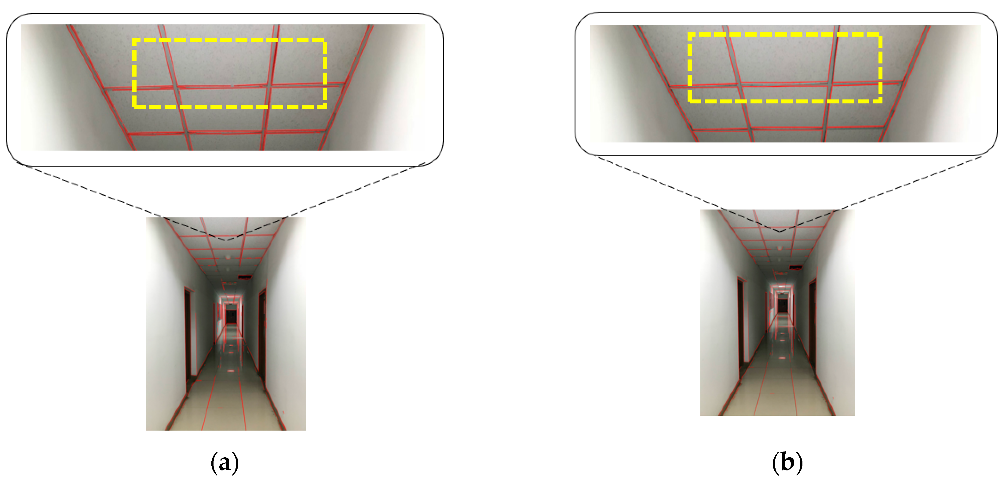
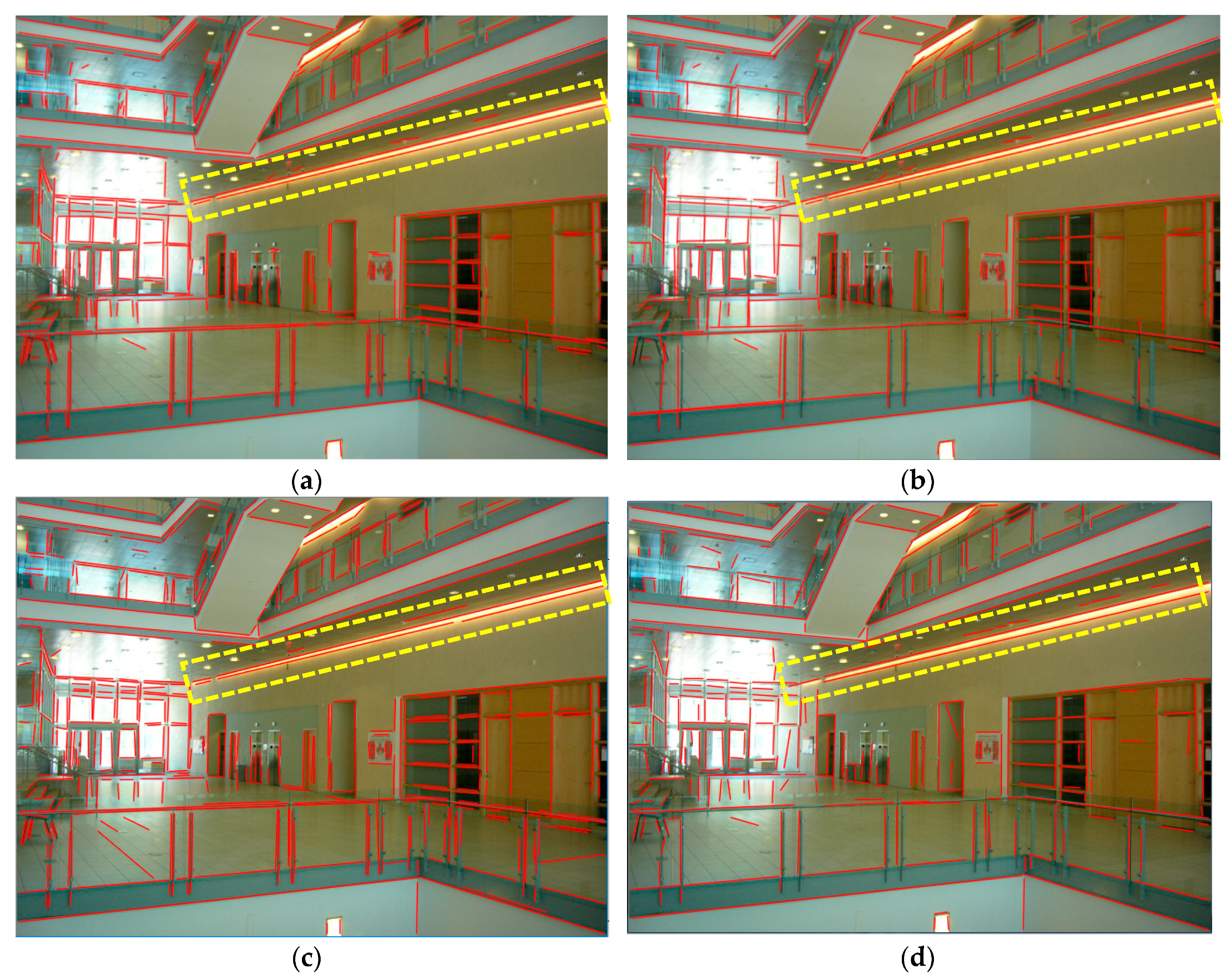
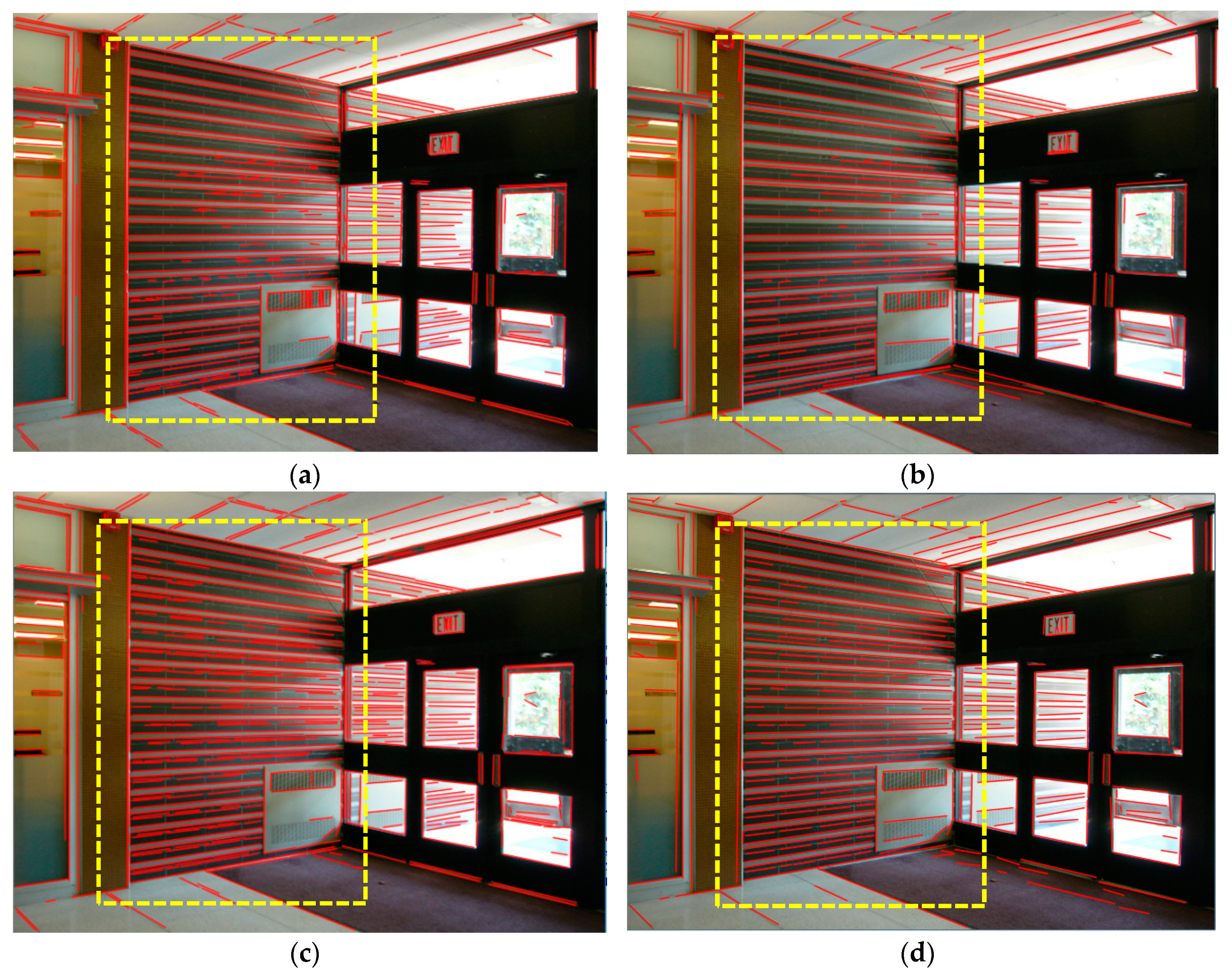
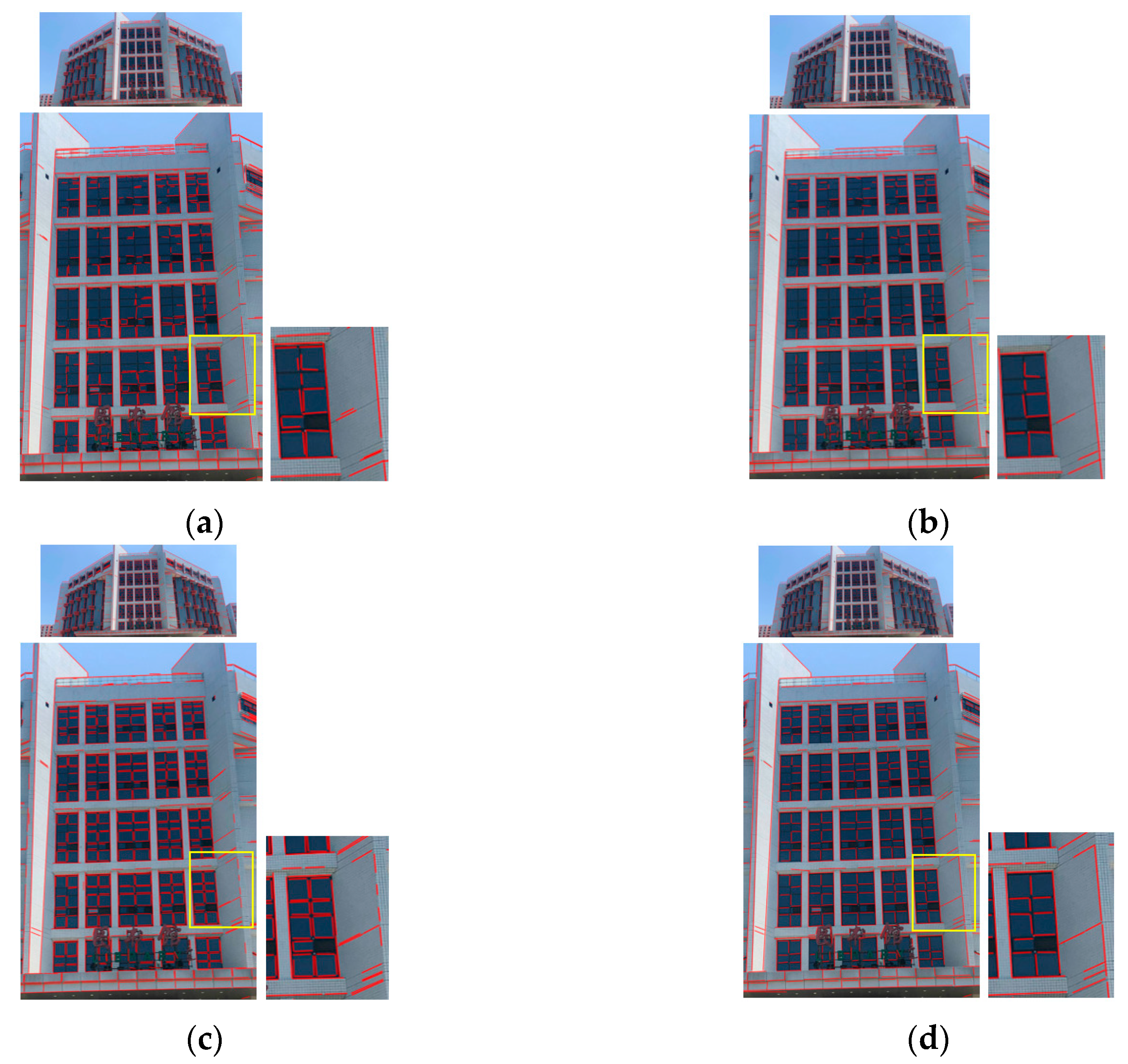
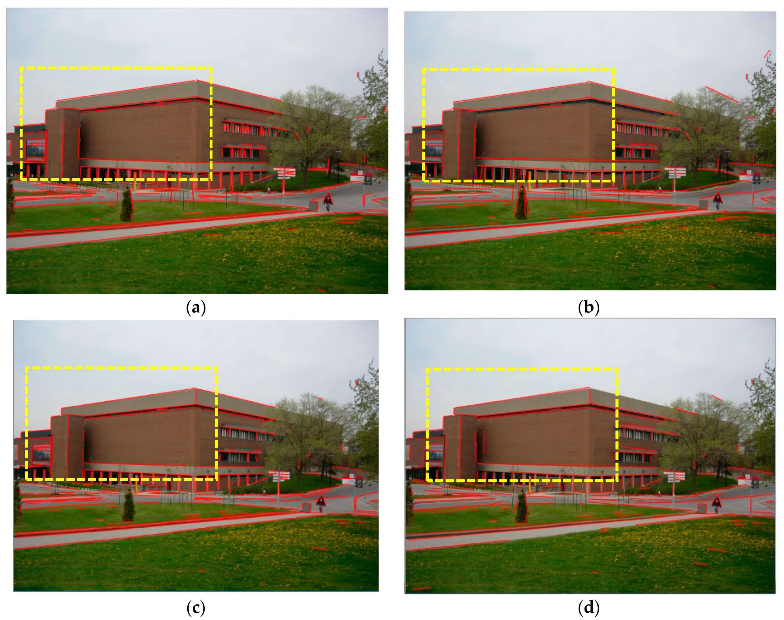
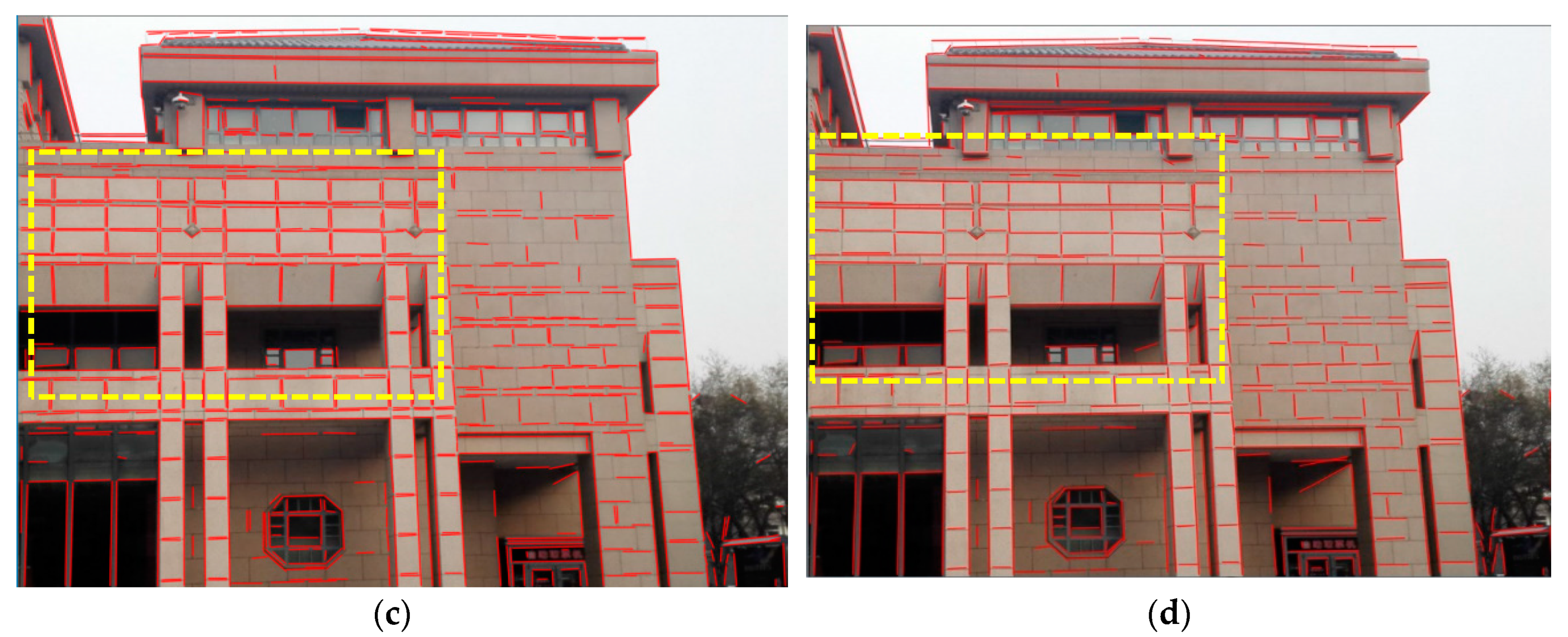
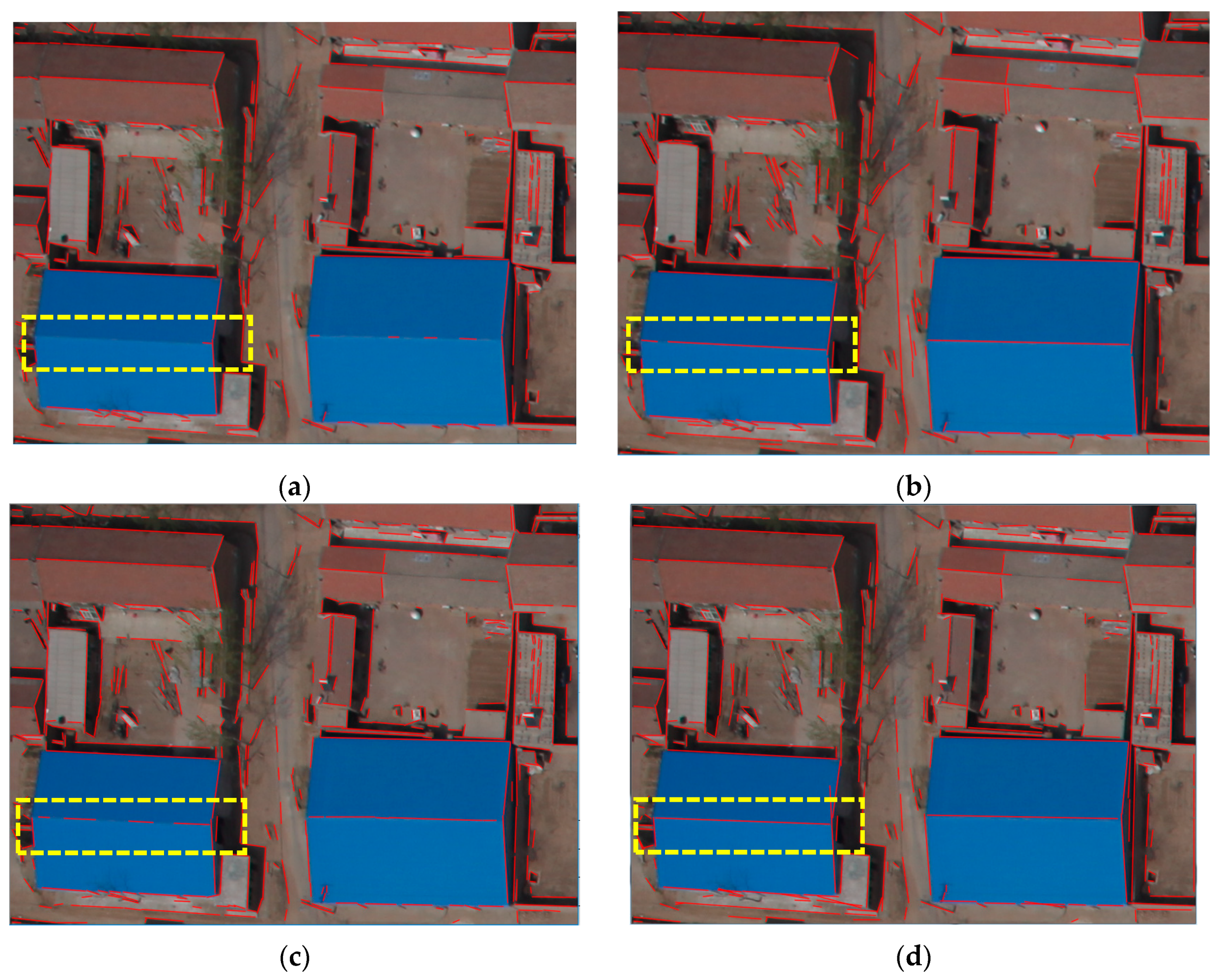
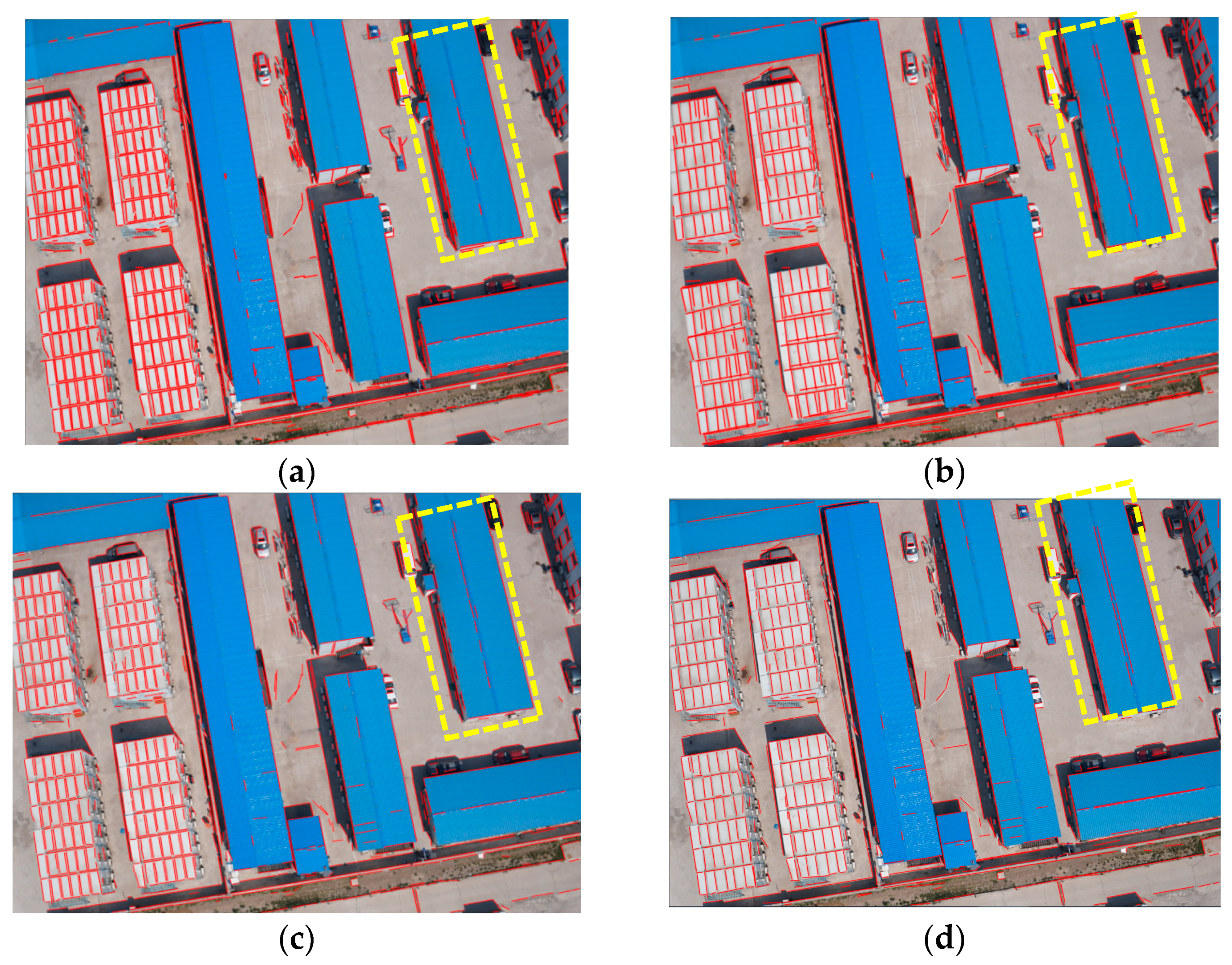
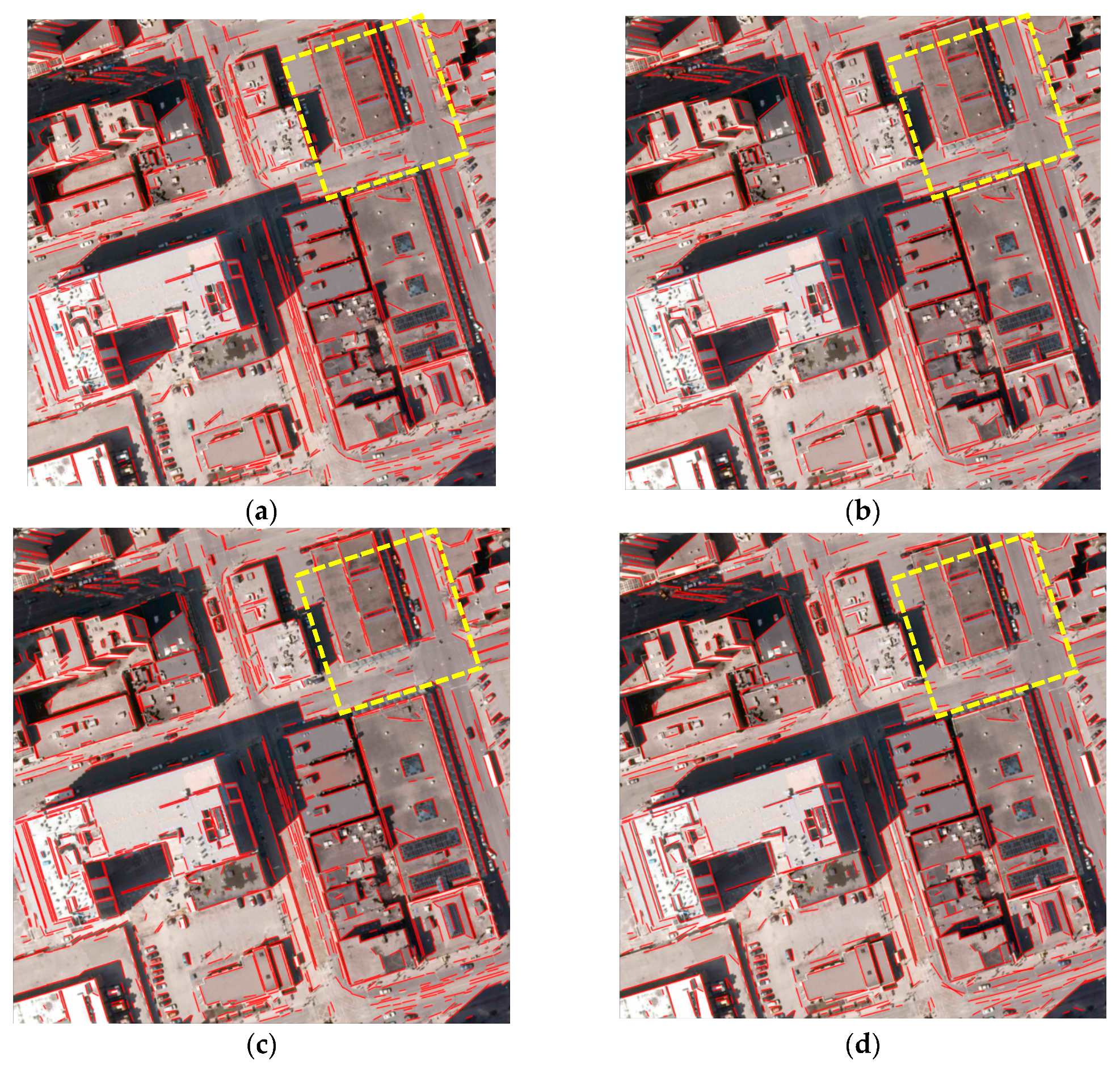
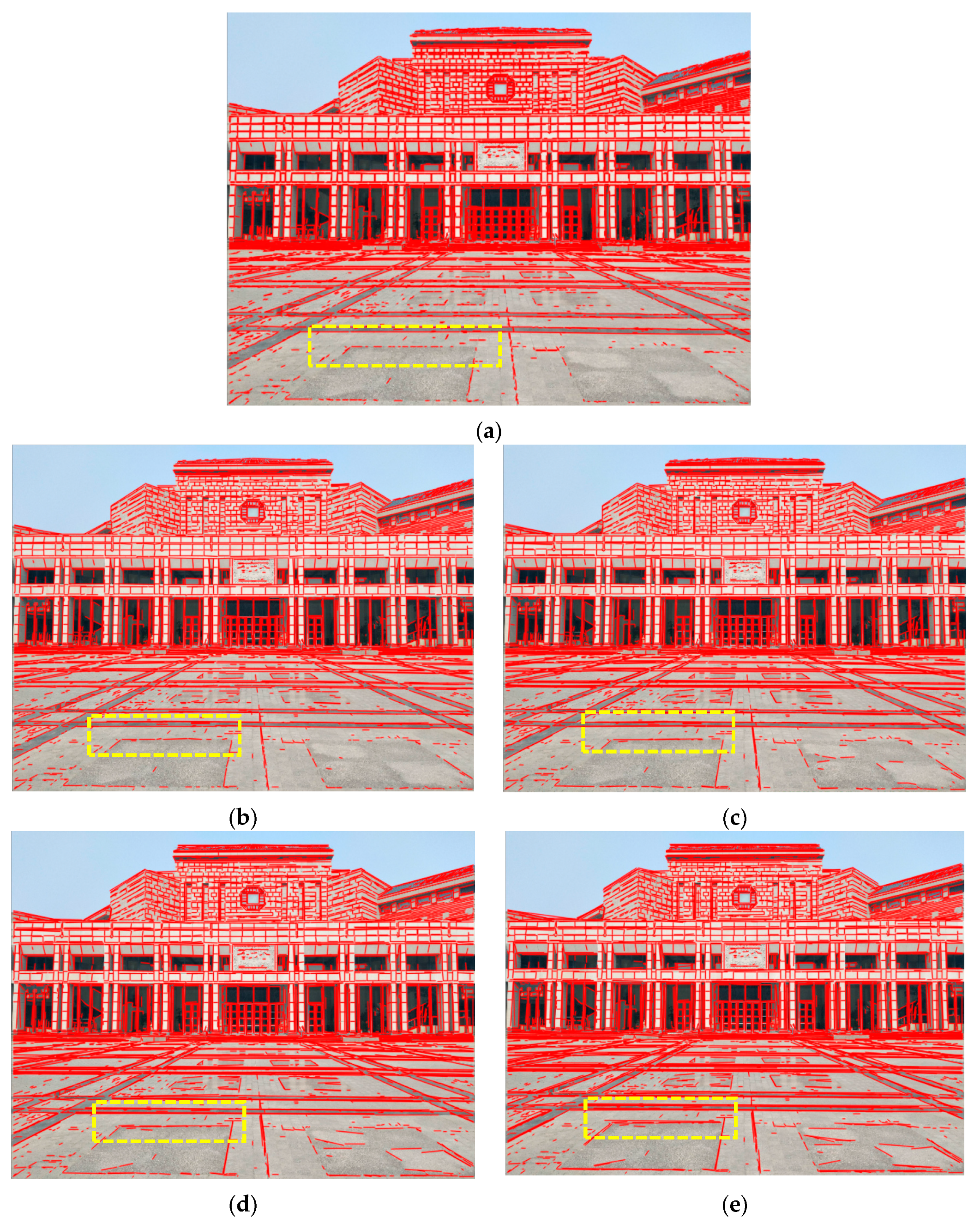
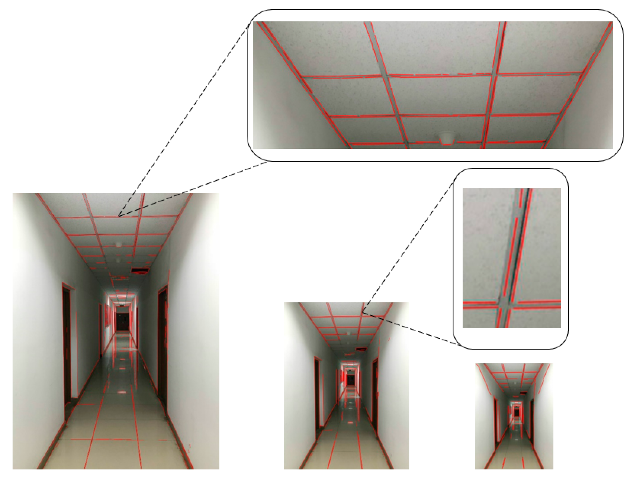
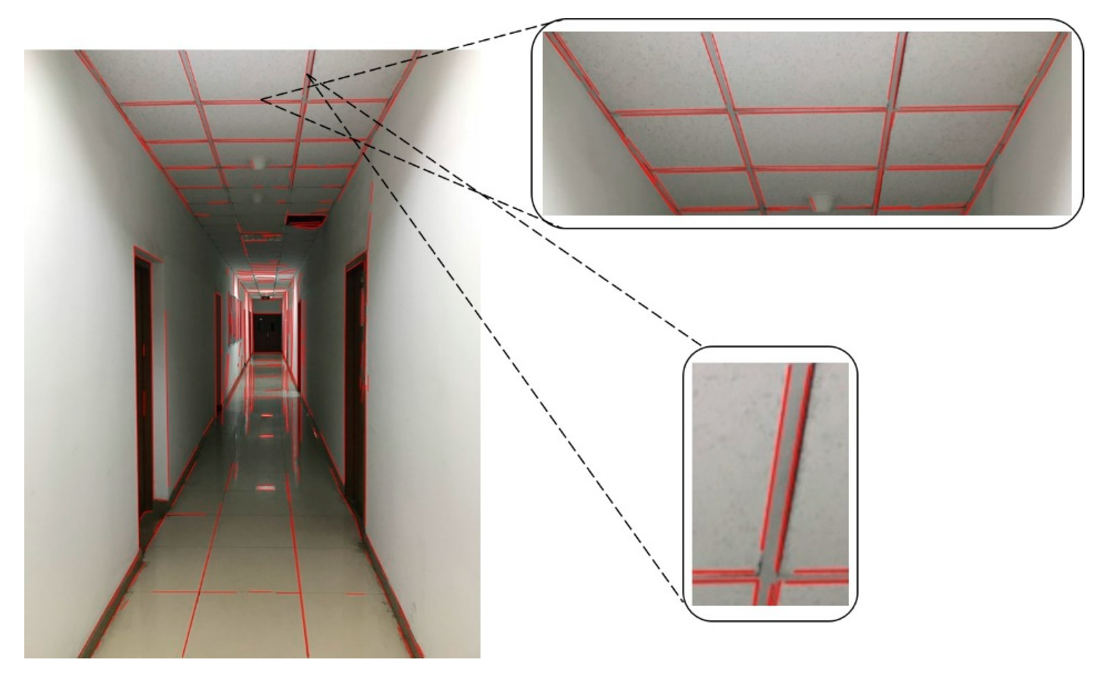
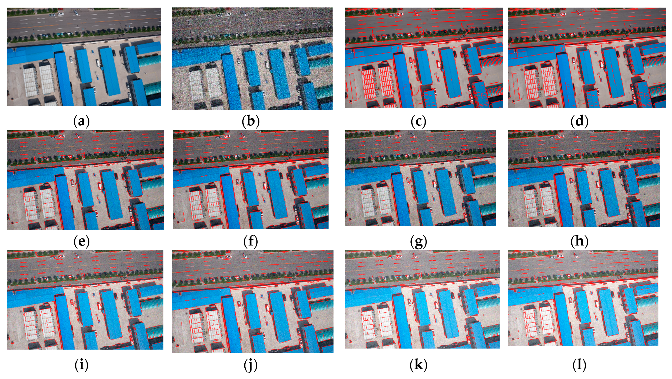
It can be seen from the visualization results in Figure 8, Figure 9, Figure 10, Figure 11, Figure 12, Figure 13, Figure 14, Figure 15 and Figure 16 that the proposed methods MSLSD and MSEDLines alleviated the segmentation fracture effect of line segments. Also, it can be seen from the local area marked by the yellow frames in the nine figures that the line extraction results of conventional LSD and EDLines method were affected by image factors such as grayscale distortion, causing a relatively severe fracture phenomenon. MSLSD and MSEDLines had the effect of optimization and could merge multiple broken short line segments into one complete long segment. Additionally, we can clearly see from Figure 9, Figure 10, and Figure 13 that the proposed methods, MSLSD and MSEDLines, played a role in removing redundancy, eliminating the redundant lines while retaining the key geometric contour lines. From the comparison of Figure 10a,b, it was found that the proposed method MSEDLines could remove some pseudo-lines extracted by algorithm mistakes.

Table 1 shows the quantitative results of line extraction with nine sets of experimental data of indoor, outdoor, and aerial images. Regardless of indoor or outdoor environments or aerial scenes, MSLSD and MSEDLines extract longer lines than the corresponding traditional methods, LSD and EDLines. The longer the average length of line segments, the higher the integrity of extracted line segments on the images. For Indoor 1, the line segment average length of MSEDLines and MSLSD was 85.3 pixels and 85.2 pixels respectively, which is much higher than that of EDLines (63.1 pixels) and LSD (51.3 pixels). Since our methods had the effect of removing line segment redundancy, the number of extracted line segments was less than that of conventional methods. MSEDLines and MSLSD extracted 215 and 238 line segments respectively from Indoor 1, while EDLines and LSD extracted 327 and 445 line segments, respectively. However, the reduction in the number of line segments does not result in the sharp drop in the total length of line segments. Because proposed methods in this paper preserve and optimize the key geometric contour information on the image while removing the redundant line segments, they ensure that the total length does not change much. The extraction time of the four methods of MSEDLines, MSLSD, EDLines, and LSD is not much different, which indicates that the optimization steps in this paper’s algorithm did not take much time. The quantification results of line segment extraction of the other eight sets of data have the same trend as Indoor 1.

Generally, line segments extracted by MSLSD and MSEDLines were more complete than that extracted by traditional methods and they also alleviated the line segmentation fracture problem. Many broken line segments were optimized to be combined into a complete line feature, which completely expressed the geometric profile information of the target. Meanwhile, the proposed method eliminated redundant clutter in the line feature detection process. Quantitative results showed that the average length of optimized line segments extracted by the proposed method was greatly improved compared with that extracted by traditional methods. Also, it was found that the accuracy of traditional methods and proposed methods was very high, except for images including the presence of trees and reflections, for example, such as Indoor 1 and Outdoor 2, and the accuracy of the proposed method was generally higher than that of the classical method. The line feature extraction time of all four methods in the paper was similar. The proposed method does not affect the extraction efficiency.

4. Discussion

4.1. Parameter Setting

This part discusses the selection of problem-oriented parameters in the model construction process, providing the basis for constructing the most suitable multi-scale image space model for various resolution images. The image resolution is different, as is as the maximum number of down-sampling setting, which causes the number of multi-scale image space model layers formed to be different.

In order to get a suitable multi-scale image space for a line feature extraction, the corresponding and reasonable maximum down-sampling number t_max should be set according to the image resolution. Regarding the construction of multi-scale image space, this article is consistent with the traditional empirical method. The scale space factor σ is 0.5 and the whole model has a total of N-layered images. To discuss the selection of model parameteres, an outdoor image (front view of the Grand Auditorium) with a resolution of approximatly 10 million pixels (3500 × 2625) was used as an example to down-sample from one to four times. The corresponding multi-scale image space model was constructed and the line features of the image were extracted by MSLSD. The results are shown in Figure 17 and

Table 2. MSLSD line segment extraction results under different down-sampling times.

Down-sampling Times	Resolution	The Number of Line Segments	Time-consuming (s)	Average Length (pixel)
0	9187500	8248	6.138	53.0
1	2296000	4273	8.440	79.8
2	574000	4191	8.836	92.9
3	143664	4251	8.998	103.3
4	35916	3393	10.574	110.4

.

As we can see from Figure 17a, a line segment extracted from the original image suffers a severe fracture effect. Using our proposed method to construct a multi-scale image space model, we can effectively alleviate the fracture problem of extracted line segments, as can be seen from Figure 17b–e and Table 2, and the average length of the line segments is greatly improved. The continuity of line segment extracted by MSLSD with fusion of down-sampled images becomes better, but with the increase of down-sampling times, images, particularly those down-sampled four times, do not change the effect of extracted segments much. Moreover, the average length of line segments changed from 103.3 to 110.4 pixels, which shows that the growth trend was not obvious. Therefore, to construct the multi-scale image space model, we set model parameters according to the proposed rules of

Table 3. The setting rules of model parameters.

Size	Large Resolution	High Resolution	Medium Resolution	Low Resolution
	σ = 0.5
Pixels	>107	106–107	105–106	<105
tmax	>3	3	2	1
N	>4	4	3	2

.

The super-resolution images of more than 10 million pixels were down-sampled at least three times to form more than four layers of the multi-scale image space model. High-resolution images with megapixel resolution were down-sampled three times to form an image pyramid model of four-layered multi-scale image space. Mid-resolution images were down-sampled twice to form a three-layered pyramid-like model. Low-resolution images with a pixel resolution of less than 100,000 pixels only needed to be down-sampled once to form a two-layered scale image space.

4.2. Extraction Error Analysis

Taking the indoor corridor image as an example, when MSLSD constructs a multi-scale image space model and uses LSD algorithm to extract line features from down-scaled space, the extraction error of line features on the down-sampling image is larger than that on the original image. As is shown in Figure 18, Gaussian blur makes the image resolution lower; this is an indispensable step of model construction, causing the extraction error to be amplified.

In the optimization and purification process, the proposed MSLSD method always takes the line segment on the original image as the reference, ensuring the extraction error from the low-resolution image is not introduced. Figure 19 is the result of MSLSD optimization, where we can see the method of this paper solved the line segmentation problem and ensured the accuracy of the final extracted line segments.

Therefore, selecting the line segment extracted from the original image as the benchmark in the optimization and purification process can ensure the line segment extraction accuracy. It does not introduce additional error generated by the low-resolution image line segment extraction when constructing the multi-scale image space.

4.3. The Impact of Image Noise

Image noise tends to affect line segment extraction and causes serious line segmentation fracture problems. In order to analyze the influence of the proposed method on noise, we selected an aerial image with a resolution of 1440 × 920 for discussion. In the experimental analysis, the image was down-sampled twice, forming a three-layer multi-scale image space. Simultaneously, we added Gaussian white noise with different mean and variance to the image. We found that, when the noise variance was greater than 0.02, the image quality was seriously affected. Based on this, the traditional and proposed methods under different image noises with means of 0, 0.1, and 0.2 and variances of 0.005, 0.01, and 0.02 were analyzed. The partial line segment extraction result of the noisy image is shown in Figure 20.

The complete line segment extraction results are shown in Figure 21, which reflects the average length of line segments for several methods under different noise conditions.

Without image noise, LSD can extract 1613 line segments and the average length of line segments is 33.2 pixels, while MSLSD can detect 998 line segments and the average length of line segments is 43.4 pixels. In Figure 20, we find that the number of line segments extracted by the conventional methods and proposed methods is significantly reduced due to the influence of image noise.

Meanwhile, it can be firstly found from Figure 21 that LSD is greatly affected by image noise. The larger the image noise, the more obvious the line segmentation fracture phenomenon, resulting in the shorter average length of the line segment. Secondly, MSLSD is robust to noise and is less affected by noise. Under different image noise environments, the average length of line segment extraction is basically unchanged. The average length of the MSLSD line segment extraction without noise is 43.4 pixels and the average length of the MSLSD line segment extraction under various noise conditions is maintained at 41.2–45.3 pixels. Thirdly, EDLines is less affected by image noise than LSD, but it still produces severe line segmentation fracture problems in noisy environments. In this article, MSEDLines can also alleviate the influence of image noise on line segment extraction and the average length of the line segment is greatly improved compared to EDLines. Through the discussion, MSLSD/MSEDLines can make the average length of lines longer than LSD/EDLines under different Gaussian noise conditions, respectively.

5. Conclusions

In this article, our proposed line detection method, MSLines, including MSLSD and MSEDLines, solves the line segmentation fracture problem. This novel method has the following advantages and characteristics: (1) Using advantages of down-sampling fuzzy processing, the influence of grayscale distortion on line segment extraction is reduced and the segmentation fracture effect of the traditional line feature extraction algorithm is alleviated. The continuity of line segments is improved. (2) Multi-scale image space line features are combined to construct an optimization and purification strategy with multiple constraints. The average length of extracted line segments is longer with higher integrity. Longer and accurate line segments provide a good research basis for line-based camera calibration, image matching, and 3D reconstruction. (3) Ineffective lines with partial redundancy and pseudo-lines are removed, as well as key line segments, such as geometric contours of the main object are optimized, which makes edge structures of the image be described more intuitively and clearly. (4) Only one parameter needs to be controlled manually, which makes the novel method more automated and parameter-less.

We experimentally verified the validity and superiority of our proposed method. Compared with LSD and EDLines, our proposed method has a longer average length and higher line segment integrity, which alleviates the line segmentation fracture effect to some extent. Particularly, our approach can extract more complete and comprehensive details for structured buildings. The presented improvements also can provide better structural features for SLAM navigation and other line-based applications. However, the proposed method does not completely solve the segmentation fracture effect of line segment extraction. Later, we can consider the fusion of LiDAR (Light Detection And Ranging) point cloud data based on our proposed method to further optimize and eliminate the segmentation fracture effect of line segment extraction. It can also be considered from the classical LSD algorithm perspective to improve problems where the internal gradient direction angle of the algorithm is abruptly affected by the grayscale mutation of individual pixels, which leads to the interruption of region growing and insufficient density of the same points.