Automatic Detection of Potential Dam Locations in Digital Terrain Models


TU Wien, Department of Geodesy and Geoinformation, Research Group Photogrammetry, Gusshausstr. 27–29, 1040 Wien, Austria
*
Author to whom correspondence should be addressed.
ISPRS Int. J. Geo-Inf. 2019, 8(4), 197; https://0-doi-org.brum.beds.ac.uk/10.3390/ijgi8040197
Submission received: 27 February 2019
/
Revised: 12 April 2019
/
Accepted: 22 April 2019
/
Published: 24 April 2019
Abstract
:Structural measures for retaining and distributing water—i.e., reservoirs, flood retention and power plants—play a key role to protect and feed a growing world population in a rapidly changing climate. In this work, we introduce an automated method to detect potential reservoir or retention area locations in digital terrain models. In this context, a potential reservoir is a larger terrain form that can be turned into an actual reservoir by constructing a dam. Based on contour lines derived from terrain models, potential reservoirs are found within a predefined range of dam lengths, and the locally optimal ones are then extracted. Our method is to be applied in the very early stages of project planning and for area-wide potential analysis. Tests in a 100 km2 study area bring promising results, but also show a certain sensitivity regarding terrain model quality and resolution. In total, 250–300 candidate polygons with a total volume of more than 6 million m3 were found. In order to facilitate further processing, these are stored as a GIS vector dataset.
1. Introduction
Water has played a key role in the history of mankind. It is essential as drinking water, for irrigation in food production, and for numerous other purposes, like energy supply [1]. Consequently, water shortages are serious threats to communities or whole peoples. Compared to historic events, water shortage in the last decades is unprecedented concerning its global dimension and the number of people affected: By 2005, about 35% of the world’s population, i.e., more than 2 billion people, lived in areas of chronic water shortage [2]. Numbers are expected to increase significantly in the future with population and economic growth being the prime cause.
Other reasons are (i) the growing water demand per capita, (ii) the unequal spatial, temporal and social distribution, and (iii) the reduced water availability due to climate change [3,4]. Climate change is expected to alter the water cycle in a way that both droughts and strong precipitation will increase in intensity and frequency [5]. Especially two of the manifold impacts require tremendous efforts on a global scale in order to mitigate the consequences:
1. Natural disasters related to water—especially floods—will, by trend, grow in magnitude. It is, therefore, necessary to adapt and enhance protection measures [6,7]. Nijssen et al. [8] note a shift from flood control measures based on simulated or experienced events towards holistic risk management strategies ensuring a properly functioning, adaptive system for partly unknown future scenarios. Rieger [7] focuses on decentral measures, e.g., numerous spatially distributed retention basins.
2. Irrigation requirements will significantly increase in scope and time over the next decades [4,9,10]. In 2005, 70% of all water withdrawn worldwide was for agricultural use [11]. In some developing countries this percentage even exceeds 90% with irrigated agriculture being a substantial economic factor [4]. Although there also is considerable potential in terms of irrigation efficiency [4,9], far reaching strategies are needed to ensure drinking and irrigation water supply in a sustainable way. Extensive construction measures like dams, reservoirs and conduits will be necessary to cope with the temporal and spatial discrepancies between availability of and demand for surface water. Numerous similar projects are under way in India and China, where high discrepancies are already present today due to monsoon climate and population distribution [12,13,14].
Many of the factors influencing the decision where to build a dam—for water reservoirs, flood retention areas, power plants, or a combination of these—are related to the spatial placement and the geometry of the site, particularly in the early stages of planning [1,6].
In this work, we present an automatized method to extract potential dam locations based on a digital terrain model (DTM). The locations are optimized in terms of maximizing reservoir or retention volume while minimizing the extents of a simplified dam. The method takes into account topographic aspects to carry out an area-wide potential analysis. The results are provided as a GIS vector dataset and serve as a basis for further planning.
Related Work
There is manifold literature addressing different aspects of dam placement. An extensive review of existing research and methods is provided in [15]. The variety of scientific fields includes economic considerations [16], hydraulic modeling and potential analysis [1,17,18], but also social and environmental aspects [19,20,21]. In [22], a dynamic programming approach is presented to support decision-making in the multi-objective problem of hydropower dam placement. Many of the published approaches are also more or less explicitly related to spatial data. However, in most cases this concerns river network topology or hydraulics. The key questions are the availability of and the need for water.
Our approach complements these perspectives by primarily focusing on terrain and finding places where landscape shapes favor holding back water with minimal construction efforts. To our best knowledge there hardly is literature addressing this kind of placement optimization using digital terrain models.
[7] suggests a method to find potential flood retention basins via intersections of existing dam-like structures and river axes. Dam-like structures in this case implies both, man-made or natural structures across the river axis that could serve as extensive dams once an existing water passage through them is closed. Possible examples are railway or road embankments given their structural ability to hold back water.
This approach could basically be extended to new sites by assuming non-existing dams. However, there is an inherent limitation of the search space concerning both, location and orientation of the dam due to the dependence on a predefined river axis.
2. Methods
The method described in this paper is designed to find potential water retention capabilities on the surface of the Earth. The focus is on finding terrain shapes which favor an advantageous ratio of water retaining potential to the required structural measures. Due to the fact that the typical application of this procedure is in the very early stages of the project planning process, various simplifying assumptions are made during processing.
Specifically, the assumptions are of geometric nature. Every retention area is limited by exactly one dam building which is defined as a vertical wall with straight footprint. In height, it extends from the terrain level to the altitude of the horizontal water surface. Limitations coming from, e.g., terrain stability, hydraulic conductivity, or land use are not taken into account.
2.1. Idea and Basic Concept
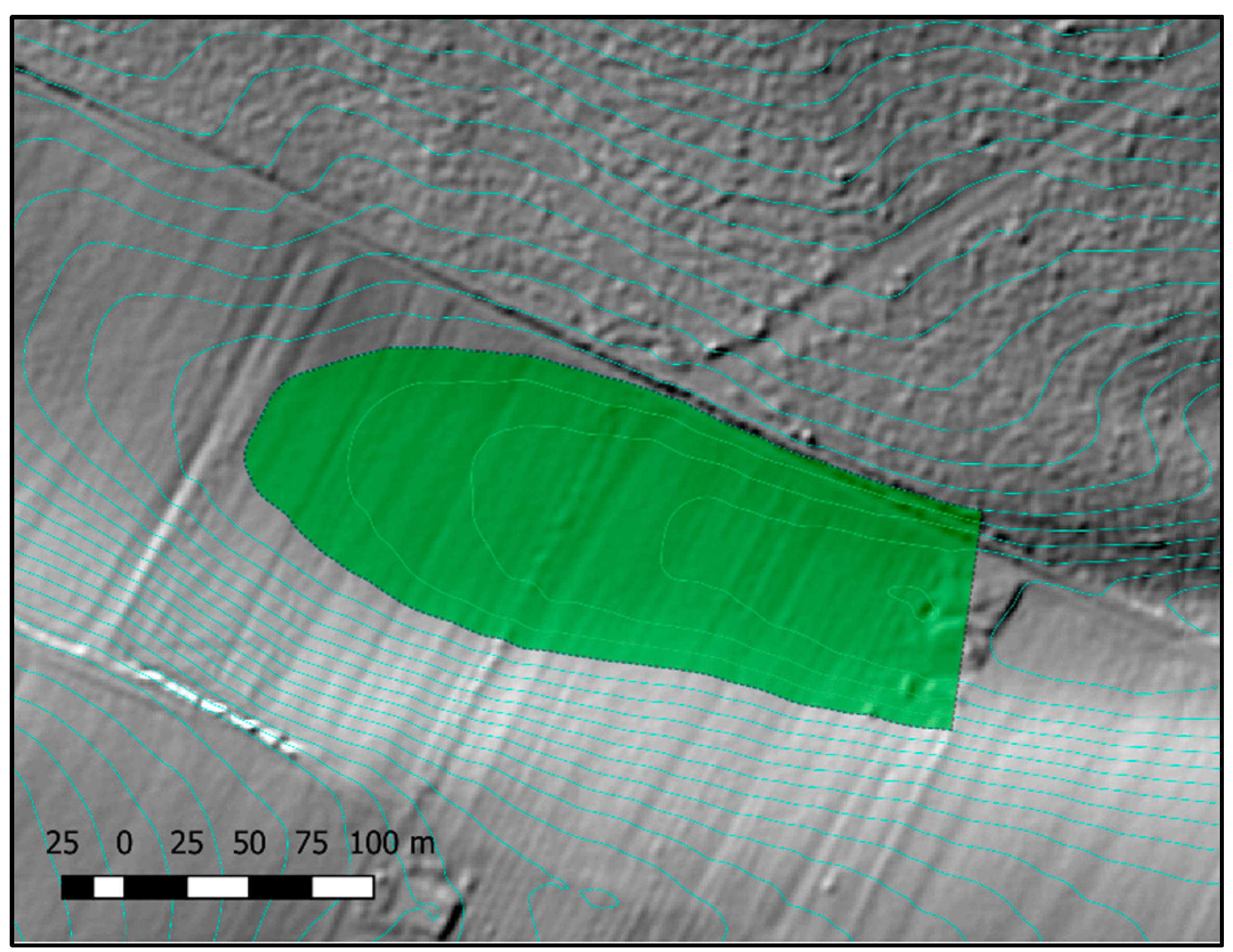
A typical location satisfying the above mentioned requirements would be a sink or a valley with an only slightly inclined axis and a sufficiently narrow passage to be closed by a dam. Having a look at contour lines, these cases are represented by a certain form: two nearby points on the line confining a long line arc in between (c.f., Figure 1 and Figure 2). The potential retention area would be limited by the contour line arc and a dam to close the remaining gap.
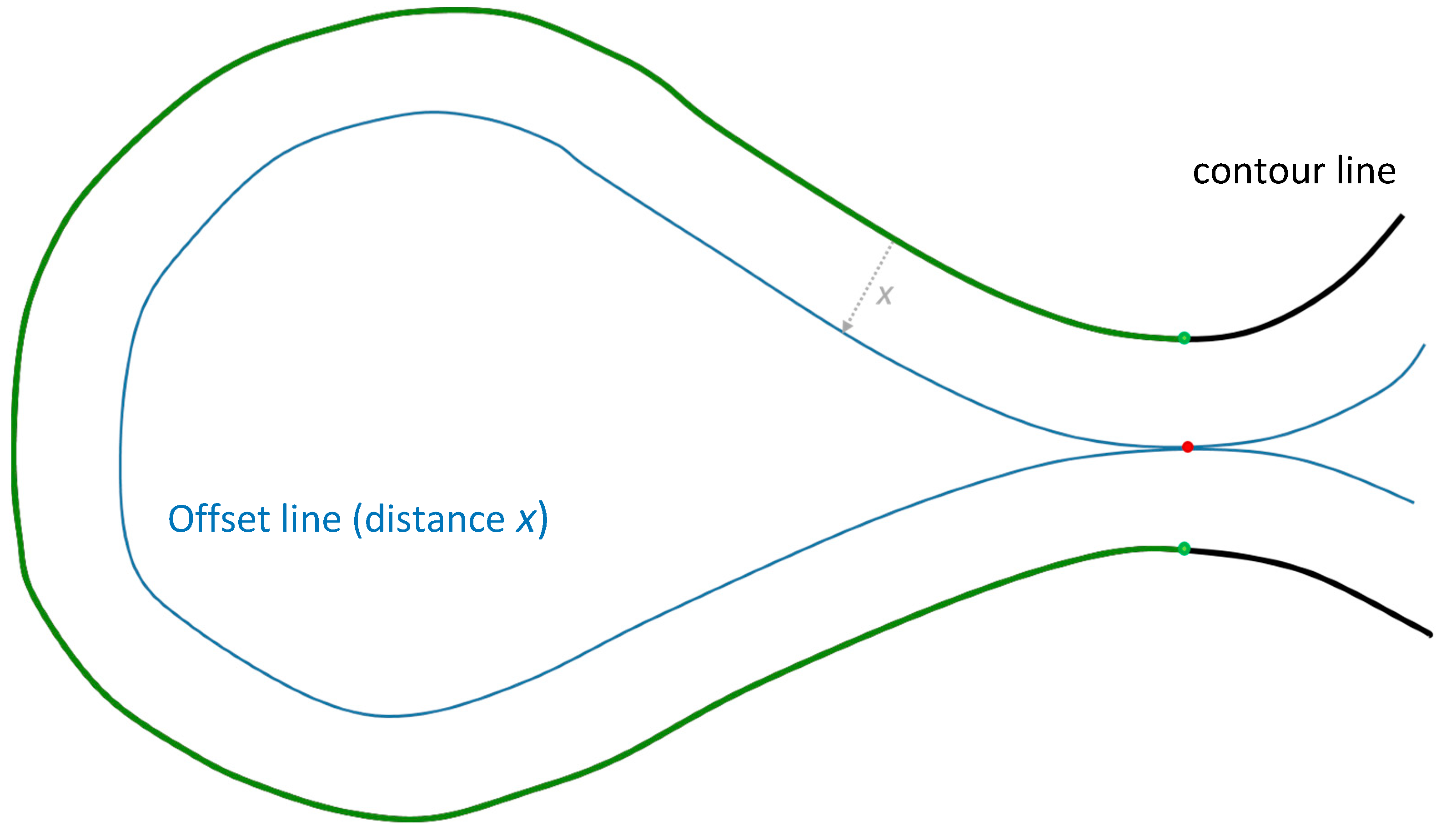
Thus, the basic idea of the algorithm is to search for these kinds of favorable segments along each contour line. This is realized by applying a parallel shift to the original line and identifying self-intersection points along the offset line. Assuming a parallel shift of a distance x, every point where two line segments of the shifted line touch or intersect indicates a location at which the contour line can be closed by a dam building of length 2x or shorter in case of intersection (c.f., Figure 2). As a second criterion, the contour line arc length has to be larger than a certain minimum in order to possibly enclose a sufficiently large area.
Obviously, if isolated 2D contour lines are regarded, not every suchlike segment indicates an expedient topography for water retention. After detection, the respective polygons therefore have to be evaluated using the DTM with regard to two criteria: (i) Is there a sufficient volume to be filled below the water level height, i.e., the height of the contour line; and (ii) is the dam height below a certain threshold defined, e.g., by legal regulations or technical capabilities?
2.2. Dam Length Optimization
Following the approach described in Section 2.1, a certain dam length has to be assumed a priori in order to set the distance for the parallel shift of the contour line. Since every potential location has its own range of meaningful or optimal dam lengths which cannot be known in advance, the implementation of this concept needs to ensure the possibility of dam length optimization.
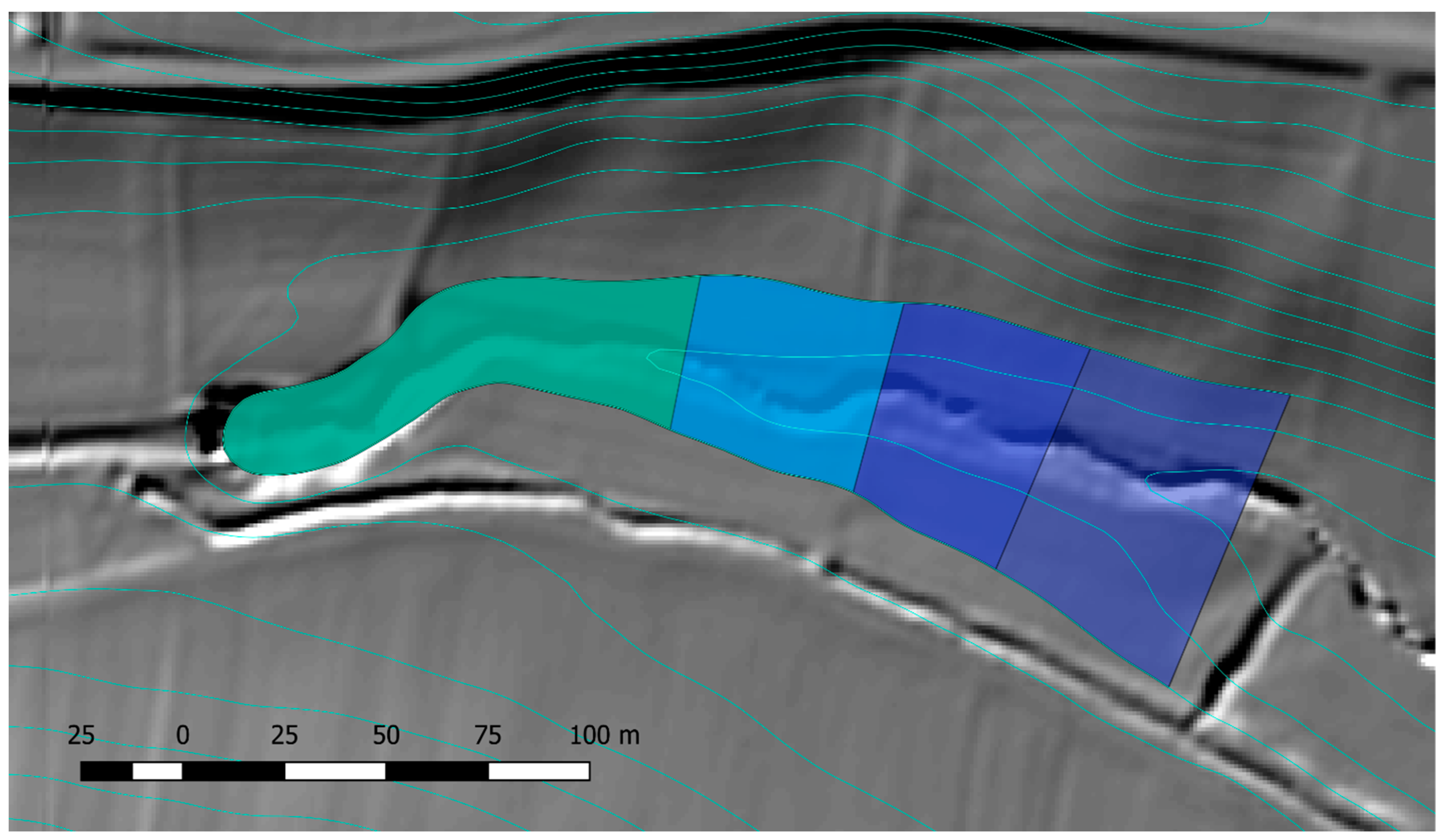
A viable solution is the stepwise application of different dam length assumptions in combination with an a posteriori filtering of the best results according to a certain quality measure. In the vast majority of cases, every polygon p(d1) detected with an assumed dam length d1 is enclosed by a polygon p(d2) where d2 > d1 (c.f., Figure 3). Consequently, if no polygon p(d2) was detected for a contour line there will be no detection p(d3) with d3 < d2 either. For the special cases where this assumption is not met, we refer to the discussion.
This suggests evaluating dam lengths in decreasing order, starting with a maximum dam length. Firstly, the search space along the contour line can be limited to a few relevant sections as a result of the longest dam analysis and secondly, if on one step no polygon is detected any more, all further ones can be skipped for the respective section. Thus, for every polygon detected in the first step, a group of extensively overlapping polygons is obtained.
Due to the fact that the polygons within one of these groups are geometrically very similar, it is possible to reduce their number prior to further processing by applying some simplified quality measure. For instance, the lake volume can be replaced by the computationally much less expensive lake area as long as a similar mean depth can be assumed. This simplification is, however, not valid when it comes to comparing polygons from all over the study area.
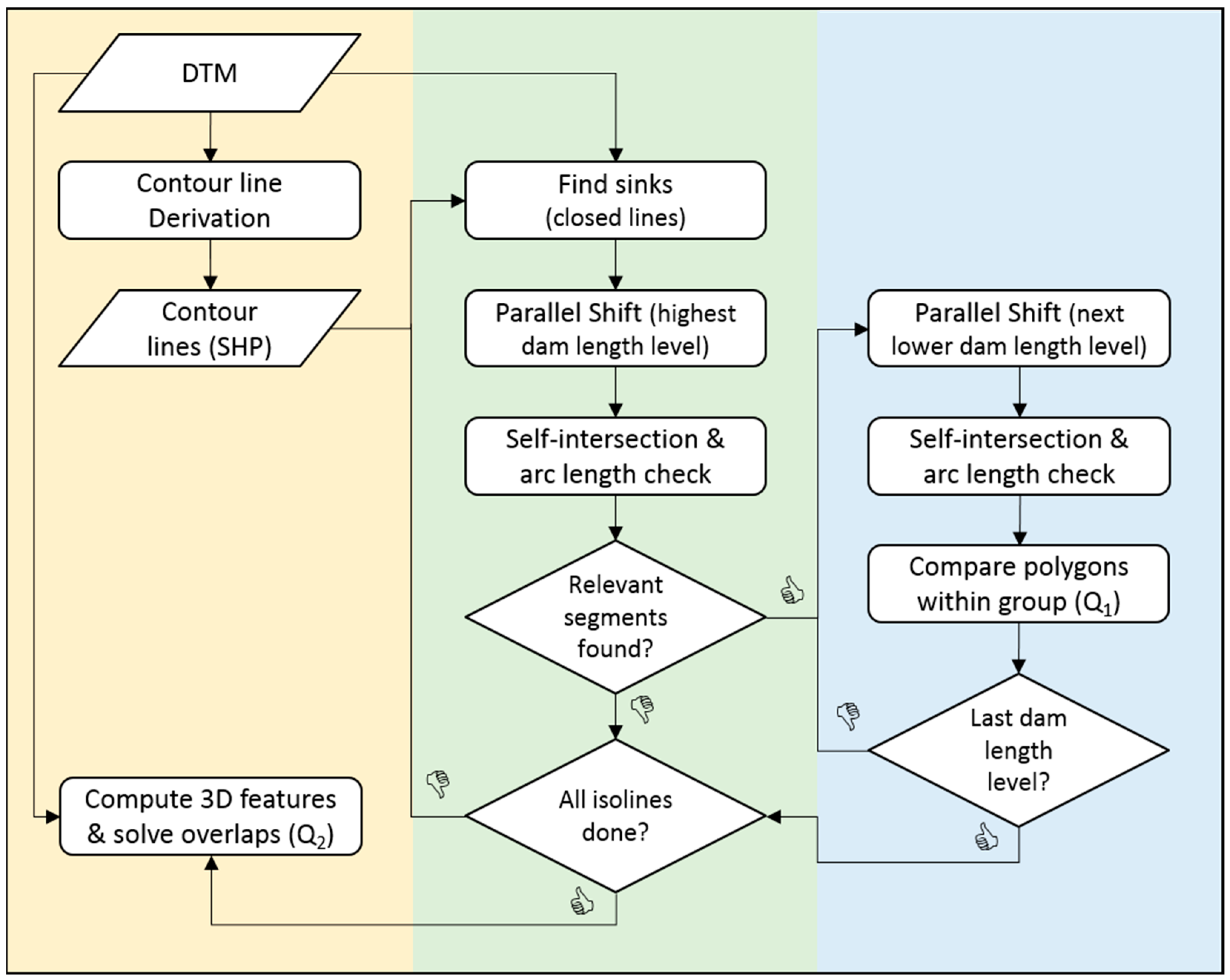
In the following section, the basic idea (Section 2.1) and the enhancement of dam length optimization (Section 2.2) are put in the context of the whole practical workflow from original DTMs to candidate retention area polygons. Figure 4 shows an overview of that workflow.
2.3. Practical Workflow
As already mentioned, the core algorithm does not use the raster DTM itself but contour lines. The source for deriving contour lines could thus also be a TIN or a point cloud representing the terrain. The first step in the workflow has to be the derivation of contour lines. In our case this was done with the “Isolines” module of the point cloud processing software OPALS [23,24]. The procedure is very similar to that offered by GDAL_contour [25]. In any case, a few parameters have to be set here which play a decisive role for the results.
First of all, a certain subset of all possible contour lines has to be designated, i.e., a height interval between the contour lines has to be set. A large value for this interval limits the search space concerning height levels, whereas a very small one offers potentially more complete results at the cost of an increased processing time. A second criterion is the resolution of the DTM from which contour lines are derived. Of course it is basically desirable to make use of the full available spatial resolution. However, depending on the algorithm, contour lines for very high resolutions (e.g., DTM raster width 1 m) tend to show a very rough behavior and a high representation complexity which potentially impinges on processing performance and the visual appearance of the results. It may therefore be reasonable to apply a slight down-sampling prior to contour line derivation. Concerning computing time, especially the contour line representation quality (points per meter of arc length) is highly relevant. Adapting this value based on the line characteristics, e.g., by thinning out points along smoother line sections, can be an efficient way to improve performance.
Using the contour lines (e.g., SHP files) as input, the detection and optimization algorithm for retention areas and the respective dams is applied. Before starting the actual detection, closed contour lines are checked as to whether they surround a sink in the terrain and accordingly no structural measures would be necessary. These candidates are directly saved as polygons with dam extents of zero meters.
The remaining contour lines are parallel shifted to both directions in 2D by half the highest possible dam length. Both directions are necessary since for an isolated contour line it is not clear, which side of the line is in uphill and which in downhill direction. It is not even guaranteed that these directions remain the same along the whole line (c.f., saddle points).
Independent from each other, the two lines resulting from every contour line are checked for self-intersections with a sufficiently long enclosed arc (c.f., Figure 2). If the arc corresponding to one self-intersection I1 completely contains the arc corresponding to another self-intersection I2, I2 is eliminated. It is also checked whether the terrain along the necessary dam building is at least partly below contour line height in order to eliminate polygons in uphill direction.
Each line arc corresponding to a valid detection defines a separate search section for the lower dam length steps, all other parts of the contour line are skipped. Once no valid detection is possible on a step, the following smaller steps—meaning shorter dams—are skipped (c.f., Section 2.2). For each of these polygon groups within one search section, the n best ones according to a simplified quality measure Q1 are kept. Assuming a similar mean depth for all polygons in one group, the area (Ar) can be used instead of the volume therefore ensuring faster processing. The respective simplified quality measure is provided in Equation 1. It relates the retention area to the dam extents, width wd and maximum height hd, thus being dimensionless. Indices r and d stand for retention area and dam, respectively. For hd, the lowest elevation of the DTM along the course of the dam is relevant.
After going through all contour lines, a set of typically strongly overlapping polygons is obtained along with their geometric features. While 2D features like lake area or dam length can be found easily based on the contour line, 3D features like retention volume or dam height need the inclusion of information from the DTM.
The most important input parameters of the described algorithm along with short descriptions are summarized in Table 1.
Basically, the resulting polygon vector data set is the most complete input for the further process. For certain applications with clear requirements, the best polygons can be extracted in a way that no spatial overlaps are given any more. Therefore, a quality measure (Q2) has to be formulated to decide on which areas are these best potential retention areas. The polygons are then sorted by this measure in decreasing order. Going through all the candidates sequentially, every less qualitative polygon overlapping with the current one is eliminated. A possible quality measure is relating retention volume (Vr) to the dam extents (width and height). This measure, however, prefers very large, shallow areas in practice. Therefore, it is subsequently scaled by the mean depth of the retention area (), i.e., the ratio of retention volume and area (Equation (2)). The unit of Q2 here is m2:
If due to legal restrictions, conflicts of interest or practical feasibility (infrastructure, accessibility, ...), certain areas are generally out of question for construction activity or water storage areas, this can be considered at two stages of processing: Either the respective areas are masked out of the DTM in the very beginning or all polygons overlapping with these areas are eliminated afterwards in GIS-based operations.
3. Study Area and Processing
For assessing the feasibility in practical applications, the method described in Section 2 was applied to a study area of about 100 km2. In order to show the respective effects, raster models with different spatial resolutions were used. The characteristics of the study area are described in Section 3.1, while Section 3.2 goes into detail concerning implementation and practical aspects. Finally, a discussion of the results is provided in Section 4. Thereby, the results from different spatial resolutions are compared also taking into account historical maps.
3.1. Study Area
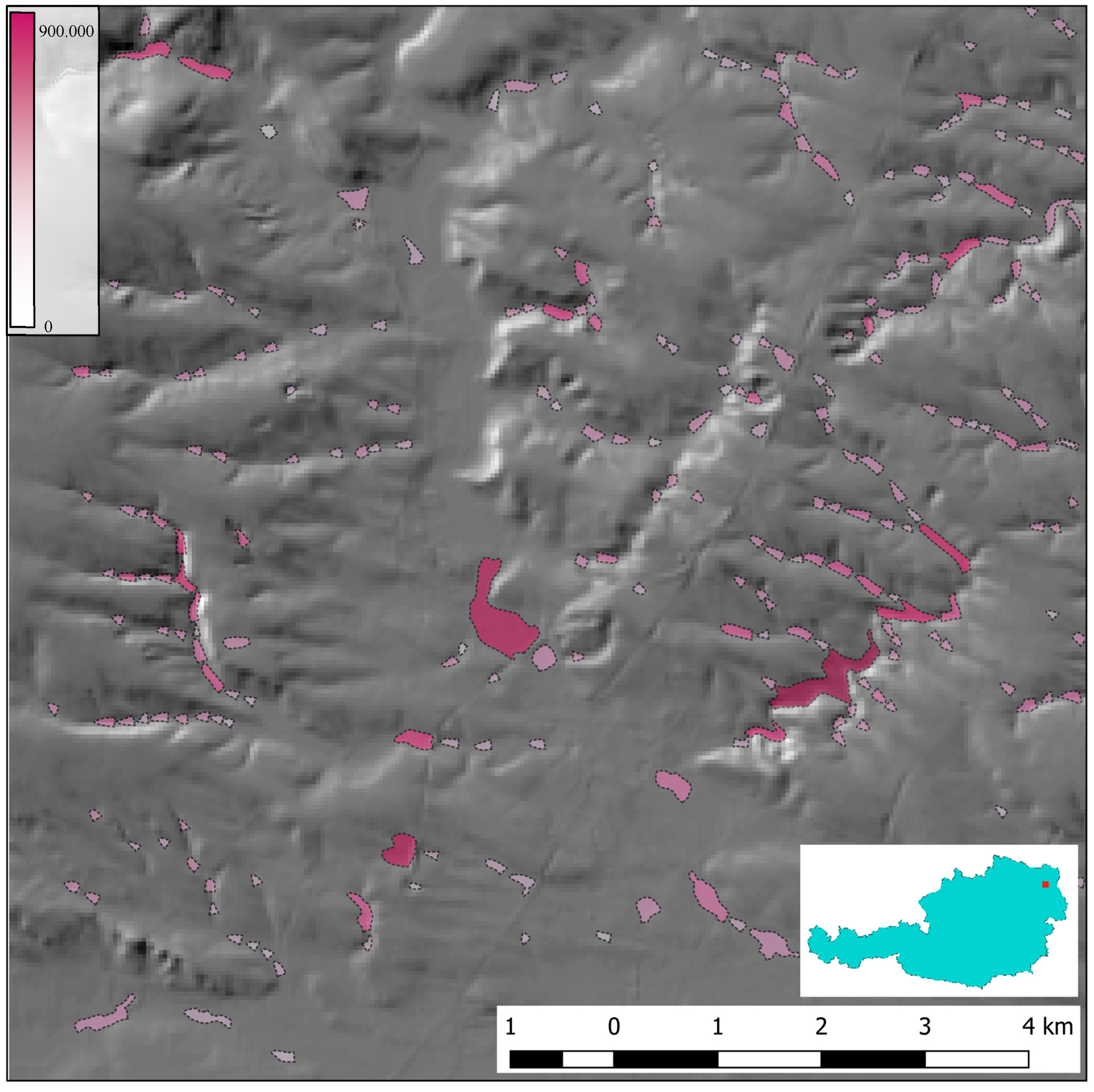
The region investigated in this study is located in the north east of the Austrian federal state Lower Austria near the town of Wolkersdorf. Situated between the foothills of the Alps and the Carpathian Mountains, the topography is dominated by rolling hills therefore posing certain challenges to retention area detection due to the rareness of sharp valleys. The study area has the peculiarity of a historic lake existing until the 19th century that was drained afterwards. Today, a part of its area is used for flood management. An overview of the study area is provided in Figure 5.
3.2. Data Processing
The dataset covering the study area is a DTM from airborne laser scanning (ALS) with a spatial resolution of 1 m. This model was smoothed using a Gaussian kernel and then down-sampled to a spatial resolution of 5 m and 40 m respectively. The 5-m-DTM was used due to the massively growing contour line complexity and processing time for the original model. Thus, contour lines were derived from the 5 m resolution DTM while features were later processed making use of the full resolution. The second spatial resolution of 40 m was chosen since it is similar to the EuroDEM [26] for Europe with a resolution of 2 × 2 arc seconds, i.e., about 40 × 60 m in central Europe, and the SRTM-1 [27] with about 1 × 1 arc second. Thereby, contour lines and features were both computed based on the same model. In Table 2, the resulting datasets are compared concerning dam and polygon features. The results for the 40 m model are visualized in Figure 5.
The raster down-sampling and the contour line deviation were both performed in OPALS (c.f., Section 2.3). The further workflow was implemented partly in Matlab (contour line analysis and detection of polygons) and Python (extraction of the best polygons). The respective processing time varies strongly with the DTM spatial resolution and also with the contour line representation complexity.
4. Discussion
As long as the underlying assumptions are fulfilled, the algorithm is able to detect valid polygons based on contour lines. Assumptions on the one hand concern the definition of contour lines and their capability to represent terrain and on the other hand the dam length steps—more precisely the expectation that every polygon on a smaller step is enclosed by another polygon from a larger step (c.f., Section 2.2). This is primarily not the case for contour lines which never open wider than the highest dam length due to borders of the study area. For the completeness of the results it is thus essential to provide contour lines spatially exceeding the area of interest and to use large overlaps for tile-wise processing. Moreover, the assumption of closing every polygon with only one dam building potentially leads to an omission of suitable locations (c.f., outlook in Section 5).
For the detected polygons, it is hardly possible to formulate quantitative quality measures. In view of the contour lines, these fit perfectly and fulfil the a priori criteria. However, quality in the sense of suitability for a given planning task depends mainly on two questions: (1) How well is the physical surface represented by the DTM, and (2) how well is the DTM represented by the contour lines? This question does not exclusively concern resolution but also the data acquisition techniques and sensors, the methods used to derive successive products (DTM, contour lines) and also the ability of the data structure to store all relevant information (e.g., bridge representation in 2.5D models). The presented method is not inherently limited to any spatial resolution or dam extent. Concerning input data the only limitation is whether these can be well represented by contour lines. It is, thus, very important to select the parameters (Table 1) and the input data in accordance with the given study area and the intended project size.
The comparison of different spatial resolutions shows good agreement in many areas but also significant differences in others. Generally speaking, a low spatial resolution or low contour line representation quality is most problematic for flat areas and small polygons where minimal terrain features may have a significant impact on polygon delineation. Consequently, if these small features cannot be represented, the effects on the result are more decisive than for large polygons in mountainous areas.
This dependency on spatial resolution and terrain characteristics can be observed in Figure 6, Figure 7 and Figure 8 where the different results are compared for various parts of the study area. Not having the possibility to profit from favourable small-scale terrain features like valley constrictions, the polygons resulting from the 40 m model are less efficient with clearly more extensive dams limiting similar or only slightly larger retention areas (q.v. Table 2). This can be seen for the smaller lake in Figure 7. The dam in the 40 m model would be placed where actually a sharp natural barrier is visible for higher resolutions. Contrarily, the undulating terrain in Figure 8 results in much smaller differences concerning dam length and placement.
The second decisive quality criterion is whether the DTM (or spatial dataset in general) can be sufficiently well represented with contour lines. In that context, the algorithm used for contour line deviation plays a decisive role along with DTM properties. Like for DTM resolution, precaution is required not to lose important small-scale terrain features—especially since the presented method has the nature of treating single contour lines in an isolated way. This is advantageous since all possible line modifications pose no problems to the workflow even though possibly changing the topology of the contour lines with respect to each other. The negative side-effect is that no control is provided as to whether the terrain is still represented well enough by the contour lines.
Further limitations from conflicting use, geology, infrastructure, hydraulics, technical construction or other factors are not considered in the very basic approach. Nevertheless, the provision of the results as polygons in a vector layer allows for integrating potential restrictions in the course of the further planning process—especially those having any kind of spatial reference.
Another aspect deserving attention is that this algorithm does not work on DTMs represented as raster [28], TIN [29], or curved patches [30], but on contour lines. Contour lines used to be the standard representation of terrain before raster and TIN models were developed. Those models clearly have their advantage for local operations, e.g., computing slope and aspect, as well as for visualization and intersection operations (e.g., profile computation), for volume computation and change detection. These operations profit from fast access to spatially neighboring points in either direction. The contour line, on the other hand, is a sorted description of all terrain points for one elevation. In that sense it is a more global representation, but restricted to only one elevation. Exactly this property is exploited by the presented algorithm.
5. Conclusions and Outlook
In this work, we presented a method to detect potential water reservoirs or retention areas based on contour lines derived from a DTM. The step-wise application of dam length assumptions and the introduction of individual quality criteria permit optimization of the results with respect to various requirements based on applications such as flood management, water resources management and energy generation.
A total retention potential of more than 6 million m3 was found in an undulating 100 km2 study area applying the described approach. The precise number also depends on the maximum acceptable construction effort per m3 of retention volume. The method can be applied to any other type of spatial data (e.g., point clouds) as long as meaningful contour lines can be derived from them. It is not limited to a certain spatial resolution of the input data. Nevertheless, resolution is, along with contour line representation quality, an important criterion for processing performance and output quality.
The work thus focuses on elaborating limitations resulting from coarser resolutions and on the implications for possible applications. The results show good agreement for global retention capabilities, while for individual retention areas dam placement and spatial extent may vary significantly as a function of resolution. Notably, the comparison was not limited to processing results, but also considered historic maps and prior knowledge about existing retention areas.
The original algorithm may be enhanced to ensure better coverage of the search space and to introduce further information:
- The assumption of only one dam per polygon is a certain limitation since this excludes valley constellations with an existing natural barrier in the middle as well as retention areas limited by two or more saddle points/valley constrictions. To cover all these cases, separate contour lines with the same height have to be combined to one entity which poses additional challenges to the validation of intermediate results (e.g., is a potential lake really closed to all sides?).
- Adding information about slope direction to the contour lines could significantly save processing time. For all the lines where the slope direction is the same along their entire course, parallel shift and self-intersection would only have to be done once instead of twice.
- Other factors concerning the constructional, economic and legal viability can currently only be hard constraints, i.e., a certain area is valid or masked out. For a better overall optimization, an introduction of soft constraints as quality criteria from the very beginning would be desirable.
Independent of the possible extensions, the suggested algorithm is simple to implement and allows an area-wide detection of individual water retention areas based on a digital terrain model analysis.
Author Contributions
Conceptualization: Michael Wimmer, Norbert Pfeifer, and Markus Hollaus; methodology: Norbert Pfeifer and Michael Wimmer; software: Michael Wimmer; validation: Michael Wimmer, Norbert Pfeifer, and Markus Hollaus; formal analysis: Michael Wimmer, Norbert Pfeifer, and Markus Hollaus; investigation: Norbert Pfeifer, Markus Hollaus, and Michael Wimmer; resources: Michael Wimmer; data curation: Michael Wimmer and Markus Hollaus; writing—original draft preparation: Michael Wimmer; writing—review and editing, Norbert Pfeifer and Markus Hollaus; visualization: Michael Wimmer; supervision: Norbert Pfeifer, and Markus Hollaus; project administration: Norbert Pfeifer; funding acquisition: Norbert Pfeifer.
Funding
The research was funded by the Austrian Federal Ministry for Sustainability and Tourism (BMNT). The authors acknowledge the TU Wien Library for financial support through its Open Access Funding Program.
Acknowledgments
The authors also wish to thank the LFRZ GmbH for data provision and support.
Conflicts of Interest
The authors declare no conflict of interest. The digital terrain model was provided by the funder. The study was designed in accordance with requirements formulated by the funder but without direct influence of the funder; the funder had no role in the analyses or interpretation of the data; in the writing of the manuscript; or in the decision to publish the results.
References
- Giesecke, J.; Mosonyi, E. Wasserkraftanlagen—Bau, Planung und Betrieb; Springer: Berlin/Heidelberg, Germany, 2009. [Google Scholar] [CrossRef]
- Kummu, M.; Ward, P.J.; de Moel, H.; Varis, O. Is physical water scarcity a new phenomenon? Global assessment of water shortage over the last two millennia. Environ. Res. Lett. 2010, 5, 3. [Google Scholar] [CrossRef]
- Vörösmarty, C.J.; Green, P.; Salisbury, J.; Lammers, R.B. Global Water Resources: Vulnerability from Climate Change and Population Growth. Science 2000, 289, 284–288. [Google Scholar] [CrossRef]
- Fader, M.; Shi, S.; von Bloh, W.; Bondeau, A.; Cramer, W. Mediterranean irrigation under climate change: More efficient irrigation needed to compensate for increases in irrigation water requirements. Hydrol. Earth Syst. Sci. 2016, 20, 953–973. [Google Scholar] [CrossRef]
- IPCC. Climate Change 2014: Synthesis Report. Contribution of Working Groups I, II and III to the Fifth Assessment Report of the Intergovernmental Panel on Climate Change; Core Writing Team, Pachauri, R.K., Meyer, L.A., Eds.; IPCC: Geneva, Switzerland, 2014. [Google Scholar]
- Scholz, M.; Yang, Q. Guidance on variables characterizing water bodies including sustainable flood retention basins. Landsc. Urban Plan. 2010, 98, 190–199. [Google Scholar] [CrossRef]
- Rieger, W. Prozessorientierte Modellierung Dezentraler Hochwasserschutzmaßnahmen. Ph.D. Thesis, Bundeswehr University Munich, Neubiberg, Germany, 2012. [Google Scholar]
- Nijssen, D.; Schumann, A.; Pahlow, M.; Klein, B. Planning of technical flood retention measures in large river basins under consideration of imprecise probabilities of multivariate hydrological loads. Nat. Hazards Earth Syst. Sci. 2009, 9, 1349–1363. [Google Scholar] [CrossRef]
- Fischer, G.; Tubiello, F.N.; van Velthuizen, H.; Wiberg, D.A. Climate change impacts on irrigation water requirements: Effects of mitigation, 1990–2080. Technol. Forecast. Soc. Chang. 2007, 74, 1083–1107. [Google Scholar] [CrossRef]
- Rasmussen, J.; Sonnenborg, T.O.; Stisen, S.; Seaby, L.P.; Christensen, B.S.B.; Hinsby, K. Climate change effects on irrigation demands and minimum stream discharge: Impact of bias-correction method. Hydrol. Earth Syst. Sci. 2012, 16, 4675–4691. [Google Scholar] [CrossRef]
- Siebert, S.; Döll, P.; Hoogeveen, J.; Faures, J.-M.; Frenken, K.; Feick, S. Development and validation of the global map of irrigation areas. Hydrol. Earth Syst. Sci. 2005, 9, 535–547. [Google Scholar] [CrossRef]
- Jiang, Y. China’s water scarcity. J. Environ. Manag. 2009, 90, 3185–3196. [Google Scholar] [CrossRef]
- Cheng, H.; Hu, Y.; Zhao, J. Meeting China’s Water Shortage Crisis: Current Practices and Challenges. Environ. Sci. Technol. 2009, 43, 240–244. [Google Scholar] [CrossRef]
- Ravindranath, A.; Devineni, N.; Lall, U.; Larrauri, P.C. Season-Ahead Forecasting of Water Storage and Irrigation Requirements—An Application to the Southwest Monsoon in India. Hydrol. Earth Syst. Sci. Discuss. 2018, 22, 5125–5141. [Google Scholar] [CrossRef]
- Jager, H.I.; Efroymson, R.A.; Opperman, J.J.; Kelly, M.R. Spatial design principles for sustainable hydropower development in river basins. Renew. Sustain. Energy Rev. 2015, 45, 808–816. [Google Scholar] [CrossRef]
- Lipscomb, M.; Mobarak, A.M.; Barham, T. Development Effects of Electrification: Evidence from the Topographic Placement of Hydropower Plants in Brazil. Am. Econ. J. Appl. Econ. 2013, 5, 200–231. [Google Scholar] [CrossRef]
- Möderl, M.; Sitzenfrei, R.; Mair, M.; Jarosch, H. Identifying Hydropower Potential in Water Distribution Systems of Alpine Regions. In Proceedings of the World Environmental and Water Resources Congress, Alquerque, NM, USA, 20–24 May 2012; 2012; pp. 3137–3146. [Google Scholar]
- Fecarotta, O.; Arico, C.; Carravetta, A.; Martino, R.; Ramos, H.M. Hydropower Potential in Water Distribution Networks: Pressure Control by PATs. Water Resour. Manag. 2015, 29, 699–714. [Google Scholar] [CrossRef]
- Sternberg, R. Hydropower: Dimensions of social and environmental coexistence. Renew. Sustain. Energy Rev. 2008, 12, 1588–1621. [Google Scholar] [CrossRef]
- Duflo, E.; Pande, R. Dams. Q. J. Econ. 2007, 122, 601–646. [Google Scholar] [CrossRef]
- Anderson, E.P.; Pringle, C.M.; Rojas, M. Transforming tropical rivers: An environmental perspective on hydropower development in Costa Rica. Aquat. Conserv. Mar. Freshw. Ecosyst. 2006, 16, 679–693. [Google Scholar] [CrossRef]
- Wu, X.; Gomes-Selman, J.; Shi, Q.; Xue, Y.; Garcia-Villacorta, R.; Anderson, E.; Sethi, S.; Steinschneider, S.; Flecker, A.; Gomes, C.P. Efficiently Approximating the Pareto Frontier: Hydropower Dam Placement in the Amazon Basin. In Proceedings of the Thirty-Second AAAI Conference on Artificial Intelligence (AAAI-18), New Orleans, LA, USA, 2–7 February 2018; pp. 849–858. [Google Scholar]
- Pfeifer, N.; Mandlburger, G.; Otepka, J.; Karel, W. OPALS—A framework for Airborne Laser Scanning data analysis. Comput. Urban Syst. 2014, 45, 125–136. [Google Scholar] [CrossRef]
- OPALS Developer Team. OPALS—Orientation and Processing of Airborne Laser Scanning Data, TU Wien. 2018. Available online: https://opals.geo.tuwien.ac.at/html/stable/index.html (accessed on 24 April 2019).
- GDAL Developer Team. GDAL—Geospatial Data Abstraction Library, Open Source Geospatial Foundation. 2018. Available online: http://www.gdal.org (accessed on 24 April 2019).
- Hovenbitzer, M. The European DEM (EuroDEM)—Setup and harmonization, The International Archives of the Photogrammetry. Remote Sens. Spat. Inf. Sci. 2008, 37, 1853–1856. [Google Scholar]
- Farr, T.G.; Rosen, P.A.; Caro, E.; Crippen, R.; Duren, R.; Hensley, S.; Kobrick, M.; Paller, M.; Rodriguez, E.; Roth, L.; et al. The shuttle radar topography Mission. Rev. Geophys. 2007, 45. [Google Scholar] [CrossRef]
- Ackermann, F.; Kraus, K. Reader Commentary: Grid Based Digital Terrain Models. Geoinformatics 2004, 7, 28–31. [Google Scholar]
- Mandlburger, G.; Hauer, C.; Höfle, B.; Habersack, H.; Pfeifer, N. Optimisation of LiDAR derived terrain models for river flow modelling. Hydrol. Earth Sci. 2009, 13, 1453–1466. [Google Scholar] [CrossRef]
- Pfeifer, N. A subdivision algorithm for smooth 3D terrain models. ISPRS J. Photogramm. Sens. 2005, 59, 115–127. [Google Scholar] [CrossRef]
- Biszak, E.; Biszak, S.; Timár, G.; Nagy, D.; Molnár, G. Historical topographic and cadastral maps of Europe in spotlight—Evolution of the MAPIRE map portal. In Proceedings of the 12th ICA Conference Digital Approaches to Cartographic Heritage, Venice, Italy, 26–28 April 2017; pp. 204–208. [Google Scholar]
Figure 1.
Example of a potential retention area in a DTM. The full polygon is colored green to better visualize the line arc of the relevant contour line (cyan). The background shows a shaded relief map.
Figure 1.
Example of a potential retention area in a DTM. The full polygon is colored green to better visualize the line arc of the relevant contour line (cyan). The background shows a shaded relief map.

Figure 2.
Illustration of an optimal detection. The contour line is plotted in black and the relevant line arc in green. The shifted line (blue) exactly touches in one point (red) thus resulting in an optimal dam placement of length 2×. If the lines were intersecting, the dam length would be slightly shorter.

Figure 3.
Example of detections at different dam lengths (40 m, 50 m, 60 m, 80 m) for one contour line. This is an exemplary case of a very small lake where the relative change in aerial extent is very high. For increasing dam length, the respective areas are 2900 m2, 5100 m2, 7500 m2, and 10,800 m2.

Figure 4.
Overview of the practical workflow. The three columns refer to the spatial entity where a certain processing step is applied. The first column (yellow) is done for the whole study area, the second one (green) for each contour line, and the third one (blue) for every relevant section within the contour line.

Figure 5.
Overview of the study area, its position within Austria and the processing results using the 40 m terrain model. The polygons are colored by retention volume (m3). In total, about 4 % of the 100 km2 are occupied by potential retention areas, creating a retention volume of about 0.06—0.07 m3 per m2 of total area, the precise value depending on the DTM resolution used.

Figure 6.
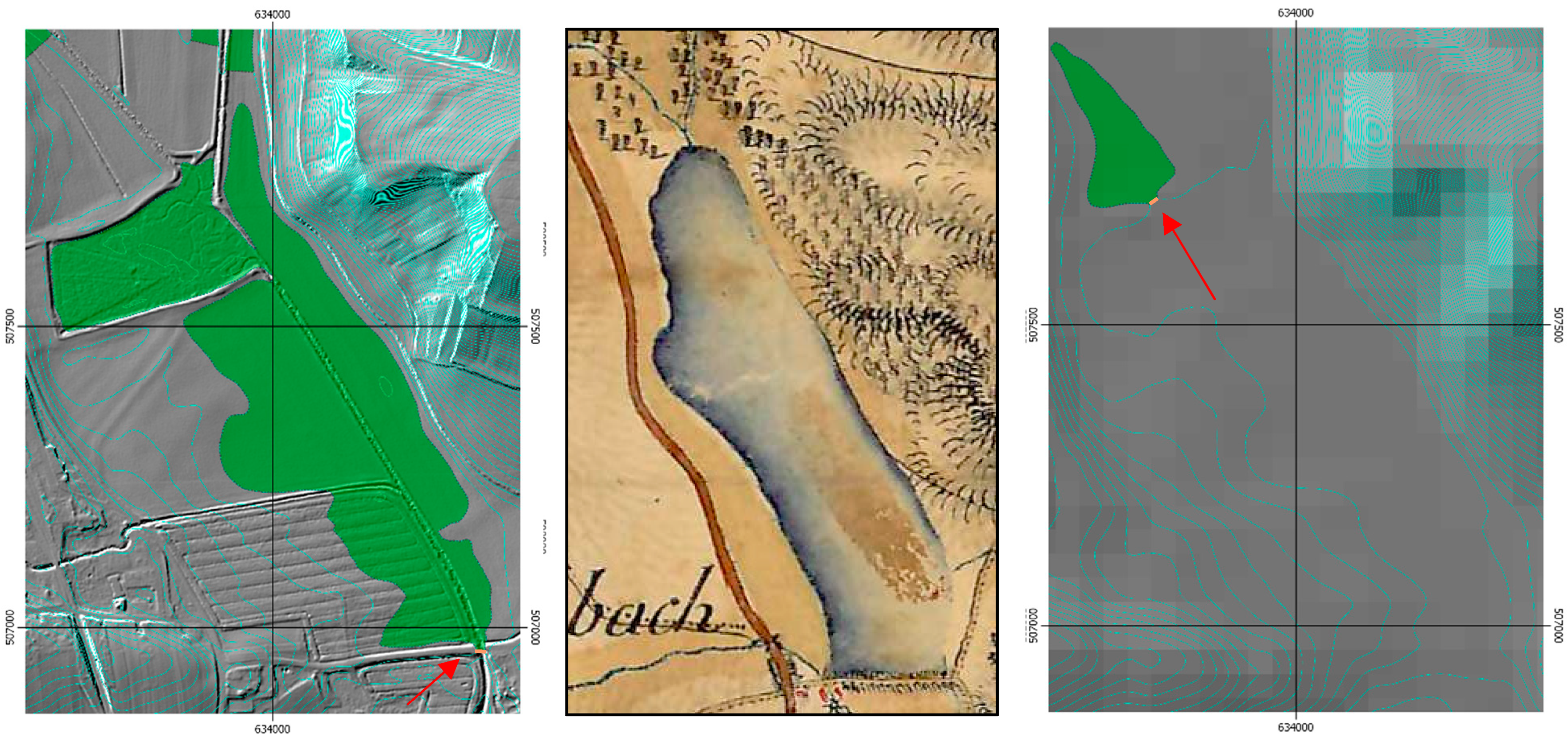
The very flat areas around a historic lake show obvious differences between the higher resolution model (left) and the low resolution model (right). In the latter one, the existing barrier at the south end is not represented thus not offering the possibility to close the retention area with a short dam (c.f., red arrows). A shaded DTM is overlaid with the contour lines (cyan), the detected polygons (green) and the dam buildings (orange). In the middle, a historic map (18th century) of the lake as provided by mapire.eu [31] is shown.
Figure 6.
The very flat areas around a historic lake show obvious differences between the higher resolution model (left) and the low resolution model (right). In the latter one, the existing barrier at the south end is not represented thus not offering the possibility to close the retention area with a short dam (c.f., red arrows). A shaded DTM is overlaid with the contour lines (cyan), the detected polygons (green) and the dam buildings (orange). In the middle, a historic map (18th century) of the lake as provided by mapire.eu [31] is shown.

Figure 7.
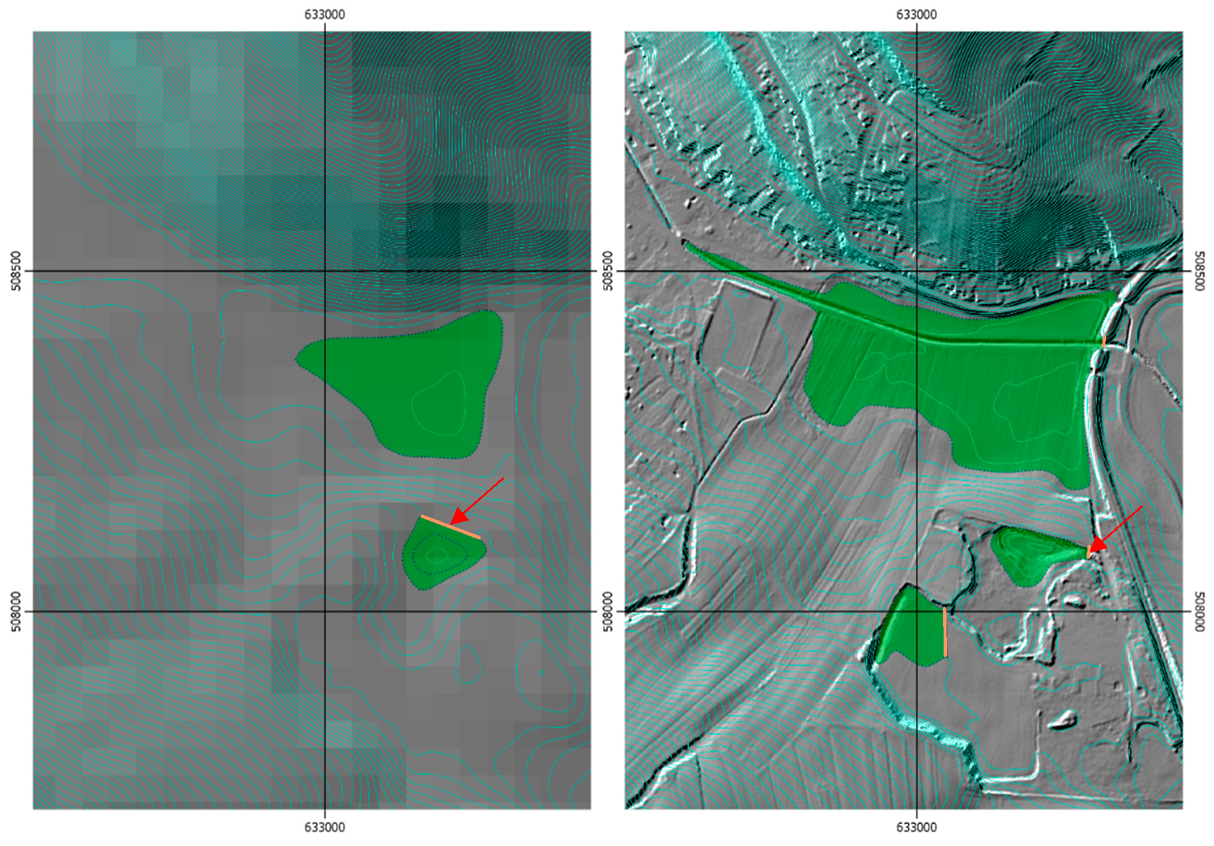
Comparison of the results in a characteristic scene of the study area. The spatial resolutions are 40 m (left) 1 m/5 m (right). The extents of the large polygon in the north vary significantly due to the smoothing in the coarser model. For the smaller polygon in the south, the extents are at least similar, but the dam is placed in a completely different way concerning both, position and extents (see red arrow). The third polygon in a very flat area is not detected in the coarse model.
Figure 7.
Comparison of the results in a characteristic scene of the study area. The spatial resolutions are 40 m (left) 1 m/5 m (right). The extents of the large polygon in the north vary significantly due to the smoothing in the coarser model. For the smaller polygon in the south, the extents are at least similar, but the dam is placed in a completely different way concerning both, position and extents (see red arrow). The third polygon in a very flat area is not detected in the coarse model.

Figure 8.
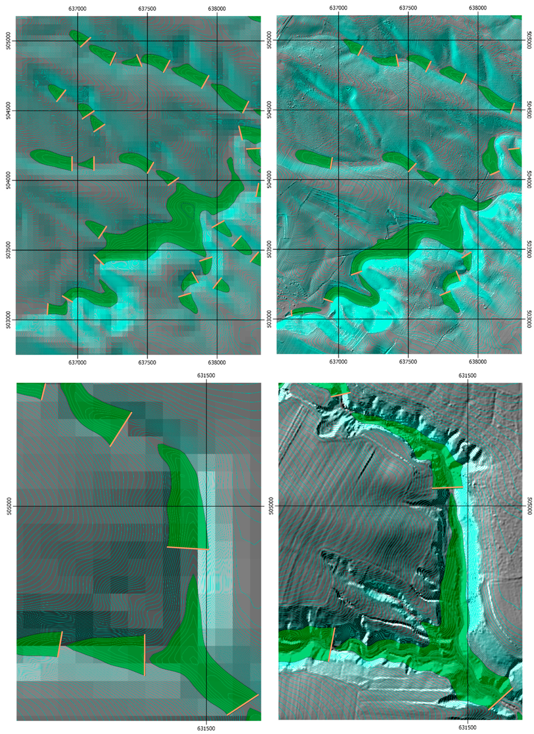
Comparison in two rather hilly regions. In the first scene, the smoother landscape shape makes the results quite similar for both resolutions, at least as far as the larger polygons are concerned. In contrast, the second scene is dominated by sharp valleys leading to clear representation differences between the two spatial resolutions and to very dissimilar resulting polygons. Notably, the 1 m/5 m model on the right is able to better resolve a local narrowing for placing a shorter dam.
Figure 8.
Comparison in two rather hilly regions. In the first scene, the smoother landscape shape makes the results quite similar for both resolutions, at least as far as the larger polygons are concerned. In contrast, the second scene is dominated by sharp valleys leading to clear representation differences between the two spatial resolutions and to very dissimilar resulting polygons. Notably, the 1 m/5 m model on the right is able to better resolve a local narrowing for placing a shorter dam.


Table 1.
The main input parameters for the detection algorithm. The given values are examples which were used for practical processing. Especially the first three depend on the spatial scale of the data and the intended project.
Table 1.
The main input parameters for the detection algorithm. The given values are examples which were used for practical processing. Especially the first three depend on the spatial scale of the data and the intended project.
| Parameter Description | Variable | Value |
|---|---|---|
| Equidistance between two contour lines | ed | 1 m |
| Dam lengths (decreasing) | damL | [100, 90,…, 20, 10, 5] m |
| Minimal arc length | minArc | 200 m |
| Number of polygons kept within a group (c.f., Figure 3) | n | 3 |
| Simplified quality measure to compare group polygons | Q1 | c.f., Equation (1) |
Table 2.
Summarized processing results for the two different resolutions (1 m/5 m and 40 m). For both, the full detection result (“all”) with n = 3 (c.f., Table 1) is compared to the selection of non-overlapping “best” polygons according to Q2 (c.f., Equation (2)). Concerning resolution, the two values describe the DTM used for feature computation and contour line computation, respectively.
| Resolution | Number of Poly. | Ø Dam Length [m] | Ø Area [m2] | Ø Volume [m3] | Σ Volume [m3] | Median (Q2) [m2] |
|---|---|---|---|---|---|---|
| 1 m/5 m all | 1979 | 60.8 | 9667 | 23,479 | - | 42.3 |
| 1 m/5 m best | 264 | 62.7 | 14,445 | 23,328 | 6.2 Mio. | 50.4 |
| 40 m/40 m all | 1968 | 81.5 | 12,126 | 22,516 | - | 40.5 |
| 40 m/40 m best | 284 | 82.0 | 15,756 | 25,243 | 7.2 Mio. | 47.1 |
© 2019 by the authors. Licensee MDPI, Basel, Switzerland. This article is an open access article distributed under the terms and conditions of the Creative Commons Attribution (CC BY) license (http://creativecommons.org/licenses/by/4.0/).
Share and Cite
MDPI and ACS Style
Wimmer, M.H.; Pfeifer, N.; Hollaus, M. Automatic Detection of Potential Dam Locations in Digital Terrain Models. ISPRS Int. J. Geo-Inf. 2019, 8, 197. https://0-doi-org.brum.beds.ac.uk/10.3390/ijgi8040197
AMA Style
Wimmer MH, Pfeifer N, Hollaus M. Automatic Detection of Potential Dam Locations in Digital Terrain Models. ISPRS International Journal of Geo-Information. 2019; 8(4):197. https://0-doi-org.brum.beds.ac.uk/10.3390/ijgi8040197
Chicago/Turabian StyleWimmer, Michael H., Norbert Pfeifer, and Markus Hollaus. 2019. "Automatic Detection of Potential Dam Locations in Digital Terrain Models" ISPRS International Journal of Geo-Information 8, no. 4: 197. https://0-doi-org.brum.beds.ac.uk/10.3390/ijgi8040197
Note that from the first issue of 2016, this journal uses article numbers instead of page numbers. See further details here.