A GIS Tool for Mapping Dam-Break Flood Hazards in Italy


1
School of Engineering, University of Basilicata, 85100 Potenza, Italy
2
Sustainable Development and Energy Resources Department, Research on Energy Systems SpA, 20134 Milano, Italy
3
Department of Bioresource Engineering, McGill University, Ste Anne de Bellevue, Quebec, H9X 1T6, Canada
*
Author to whom correspondence should be addressed.
ISPRS Int. J. Geo-Inf. 2019, 8(6), 250; https://0-doi-org.brum.beds.ac.uk/10.3390/ijgi8060250
Submission received: 3 April 2019
/
Revised: 23 May 2019
/
Accepted: 26 May 2019
/
Published: 29 May 2019
Abstract
:Mapping the delineation of areas that are flooded due to water control infrastructure failure is a critical issue. Practical difficulties often present challenges to the accurate and effective analysis of dam-break hazard areas. Such studies are expensive, lengthy, and require large volumes of incoming data and refined technical skills. The creation of cost-efficient geospatial tools provides rapid and inexpensive estimates of instantaneous dam-break (due to structural failure) flooded areas that complement, but do not replace, the results of hydrodynamic simulations. The current study implements a Geographic Information System (GIS) based method that can provide useful information regarding the delineation of dam-break flood-prone areas in both data-scarce environments and transboundary regions, in the absence of detailed studies. Moreover, the proposed tool enables, without advanced technical skills, the analysis of a wide number of case studies that support the prioritization of interventions, or, in emergency situations, the simulation of numerous initial hypotheses (e.g., the modification of initial water level/volume in the case of limited dam functionality), without incurring high computational time. The proposed model is based on the commonly available data for masonry dams, i.e., dam geometry (e.g., reservoir capacity, dam height, and crest length), and a Digital Elevation Model. The model allows for rapid and cost-effective dam-break hazard mapping by evaluating three components: (i) the dam-failure discharge hydrograph, (ii) the propagation of the flood, and (iii) the delineation of flood-prone areas. The tool exhibited high accuracy and reliability in the identification of hypothetical dam-break flood-prone areas when compared to the results of traditional hydrodynamic approaches, as applied to a dam in Basilicata (Southern Italy). In particular, the over- and under-estimation rates of the proposed tool, for the San Giuliano dam, Basilicata, were evaluated by comparing its outputs with flood inundation maps that were obtained by two traditional methods whil using a one-dimensional and a two-dimensional propagation model, resulting in a specificity value of roughly 90%. These results confirm that most parts of the flood map were correctly classified as flooded by the proposed GIS model. A sensitivity value of over 75% confirms that several zones were also correctly identified as non-flooded. Moreover, the overall effectiveness and reliability of the proposed model were evaluated, for the Gleno Dam (located in the Central Italian Alps), by comparing the results of literature studies concerning the application of monodimensional numerical models and the extent of the flooded area reconstructed by the available historical information, obtaining an accuracy of around 94%. Finally, the computational efficiency of the proposed tool was tested on a demonstrative application of 250 Italian arch and gravity dams. The results, when carried out using a PC, Pentium Intel Core i5 Processor CPU 3.2 GHz, 8 GB RAM, required about 73 min, showing the potential of such a tool applied to dam-break flood mapping for a large number of dams.
1. Introduction
Dams play an important role in water resource management by providing essential services, including the provision of potable, industrial and agricultural water, hydroelectricity, pumped storage, flood control and management, ecological outflow management, water table recharge, fishing, and aquaculture. In addition, dams also contribute in less recognized ways, including the cooling of thermal systems, river sedimentation management, ice barrier formation, anti-fire management, the creation of artificial wetlands and micro-climates, and tourism. However, as dams age, their materials degrade and they can become less functional. Moreover, as construction codes and standards change, older dams may be condemned for not meeting the current acceptable safety standards. For example, Italian legislation that was issued in 2014 (D.M. 26/06/2014), required over 500 large dams be updated to reflect the current seismic control standards in Italy. Furthermore, the effects of climate change may undermine hypotheses that previously informed the design and construction of existing dams [1]. In addition, the control and regulation of hydraulic infrastructures are not always in harmony with the evolving hydrological and sedimentological regime.
In recent years, there have been many flooding events around the world as a result of the issues described above. For example, the recent spillway failure at the Oroville dam in California required large-scale civilian evacuation due to fears regarding a possible downstream dam-break [2]. After severe seismic activity in Amatrice and Norcia, Italy (2016–2017), the integrity of the Campotosto dam was of great concern to local authorities and the surrounding population [3]. Given these situations, the study of risk related to dam failure or malfunction is a topic of urgent relevance, especially when coupled with a lack of emergency management procedures [4,5,6,7]. Therefore, it is important to map areas that can potentially be flooded as a result of a dam-break in order to understand, reduce, and manage the associated risk.
Traditional modelling approaches used to map dam break hazard areas are generally lengthy and expensive, not only in terms of the costs and technical skills required, but they can also be computationally expensive due to the simultaneous solution of the continuity, momentum and energy equations, and the large number of iterations required to achieve convergence (e.g., [8,9,10]). Parallel computing and distributed workflows are frequently used to meet the high computational demand, resulting in contemporary models becoming very computationally measured [11]. Traditional approaches remain costly and difficult to perform due to the significant amount of required data and parameters [11], despite the advances in computational power (e.g., [12]). The calibration and validation of these models are especially challenging when considering the unevenly distributed discharge and rainfall gauging stations [13]. Accessible flood risk management is especially relevant in countries where robust coping strategies and disaster management mechanisms are lacking due to limited resources or insufficient coordination between authorities [14].
It is likely that the ability to test several initial hypotheses and the ability to rapidly analyze and compare a large number of dam-break cases is of interest to decision-makers. This can be especially useful when attempting to prioritize subsequent, more detailed investigations, or for the provision of information for immediate civil protection plans. The model may also be useful for identifying critical locations and for defining the ideal computational domain for further, more detailed studies.
Given the current scenario, recent studies [15,16] have proposed novel artificial intelligence techniques, which are based on machine learning for dam break flow predictions, to overcome the limits of the above-cited traditional models. These artificial intelligence approaches have the ability to predict output data from a training and testing process, but they requires large data sets that are often not available and, therefore, are determined while using analytical results. Moreover, the methods that were proposed by Seyedashraf et al. [15,16] were not developed for mapping purposes, but for the evaluation of water depth and velocity time series. In contrast, the current study explores the development of a practical and cost-effective procedure, which is only based on easily available information and designed to delineate, through a physical-based numerical approach, the areas at risk for flooding in a dam-failure scenario.
The full procedure has been implemented in the form of a Geographic Information System (GIS) tool, with the specific aim of transferring the knowledge that is acquired from this research to the scientific and technical community, as described in Section 2. The tool’s source code is published under free and open-source licenses with end-user rights to analyze, modify, and redistribute it for any purpose. This source code is available on GitHub at https://github.com/FloodRiskGroup/SimpleDambrk. The users can contribute to, or modify, the methodologies and algorithms for further development of the technology. The design of new products, processes, applications, materials, or services based on the source code is encouraged, as this will generate new data through a community-based development process [17]. The results of the model reliability are shown in Section 4 through a comparison with historical data. Section 3 presents traditional hydrodynamic approaches on two case studies: (i) the San Giuliano hypothetical dam-break and (ii) the 1923 Gleno historical dam failure in Italy. Moreover, a demonstrative application of the proposed GIS tool for 250 Italian masonry arch and gravity dams is briefly illustrated in order to highlight the computational efficiency of the developed tool for dam-break flood-mapping. Finally, Section 5 presents the discussion and conclusions.
2. The methodological Framework
The current study presents a cost-effective GIS tool that is able to provide essential information, including: (i) the evaluation of the instantaneous breach outflow discharge for masonry dams, (ii) the analysis of downstream flood propagation, and (iii) the creation of downstream flood-prone area maps, for dam-break analysis. The tool consists of: (i) a model for evaluating the dam-break outflow hydrograph, based on analytical solutions by Ritter [18] and the Board Crested Weir model [19], (ii) downstream flood propagation, based on the numerical integration of simplified equations describing the physics of the phenomenon, and (iii) a Digital Elevation Model (DEM)-based method for the delineation of dam-break hazard-prone areas.
The GIS tool is capable of simulating one-dimensional unsteady flow using the St. Venant equations with the kinematic wave approximation, combined with wave front propagation as a monoclinical rising wave in a channel [19]. As a final result, the tool provides the peak discharge, the peak elevation, and the peak time at different distances below the dam.
The use of this tool is both rapid and economical, as it is only based on commonly available information concerning dam geometry (i.e., reservoir capacity, dam height and crest length), and a freely available online DEM, with a resolution of 90m (i.e., a Shuttle Radar Topography Mission depressionless DEM, called SRTM Void Filled DEM), provided by CGIAR-CSI (Consortium for Spatial Information) [20]. In particular, the information regarding the reservoir capacity and the height of the Italian masonry dams was gathered from the Italian Dam Register's WebGis [21], while the dam crest length data were collected from Vol. 6 of ANIDEL [22] and Vol. 7 of ENEL [23]. The information on the geometry of Italian dams was used to estimate the dam-break outflow hydrograph, while the DEM was essential for the evaluation of the downstream valley shape, specifically in terms of the valley slope and the geometry of the river cross sections. The slope is an important feature, as it affects the flood flow velocity while the river cross-sections can provide information about flood propagation in terms of wetted perimeter and area of the water flow. In this context, flood propagation was performed along the river path that was extracted using the DEM. However, due to the coarse resolution of the DEM, a freely available online vector layer of the river network (provided by the Italian National Geoportal [24]) was used to construct the topology of river network connections through the pgRouting library of PostGIS Geodatabase [25]. Therefore, the network topology consists of a set of nodes with unique identifier numbers and a set of branches for which the identification number of the upstream and downstream node is known. The topological river network layer contains four new fields: (i) 'FromNodeID' referring to the unique identifier (ID) number of the i-th upstream node; (ii) 'ToNodeID' that is related to the ID number of the i-th downstream node; (iii) 'NextDownID' associated with the ID number of the i-th downstream branch; and, (iv) 'FoceID' referring to the outlet node at the mouth of the river (e.g., closer to a large lake or on the sea).
2.1. Dam-Break Outflow Hydrograph Calculator
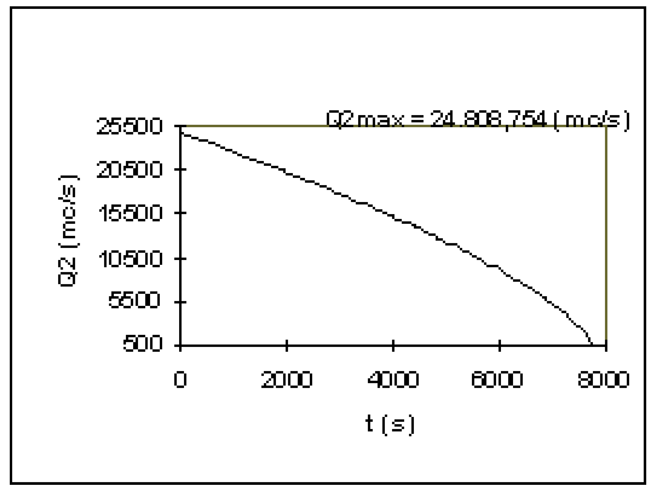
The current study focuses on arch and gravity dams and assumptions were made accordingly. Relying on the recommendation of the Italian Legislation Cir.Min.LL.PP. n. DSTN72/22806 (13/12/1995), a simplified assumption was made regarding the dam failure hypothesis. For arch dams, a rectangle with the same height as the dam and a width that was equivalent to one half the dam crest length was assumed as the branch. For gravity dams, the failure was simplified by considering a hypothesis of a rectangular breach that had the same height as the dam and a width that was equal to one-third of the dam crest length. On the basis of this consideration, the hydrograph (see Figure 1) of the outflow from the breach can be estimated by coupling two well-known methods from the literature: (i) Ritter’s [18] analytical solution for the idealized frictionless dam-break wave within a rectangular channel, and (ii) the outflow model of a Board Crested Weir. Raders may refer to [26] and [19] for a complete description of the above methodologies.
We refer to the scheme of Ritter [18] to estimate the first part of the outflow hydrograph. This scheme results in the generation of a water height that is equal to 4/9 of the dam section:
where, is the critical water depth and is the initial water depth. Therefore, we can obtain a maximum discharge equal to:
According to this theoretical scheme, water height would remain constant over time if the upstream channel were infinite. However, in reality, the negative wave, which travels back upstream, is reflected by the edge of the reservoir and it returns in the direction of the breach. At this point, water flow starts to decrease. For simplicity, this effect has been represented by the outflow model of a Broad-Crested Weir.
The outflow discharge at a specific time, which is estimated according to Ritter [18], is equal to the discharge estimated with the outflow model of a large-scale weir. Therefore, the dam water high will reach a value ; at this point, the outflow discharge is calculated while using the following formula, according to the outflow model of a Broad Crested Weir, where Critical Depth and g is the module of gravity force:
2.2. Flood Propagation Calculator
The simplified flood propagation model that is described in this study is based on methods that are proposed by Hunt [27] and improved upon by Molinaro and Fenaroli [28]. It consists of a combination of the kinematic model and propagation of steep waves theories.
It is possible to evaluate the downward attenuation of the peak discharge and a decline of the front velocity for a descending hydrograph using a combination of the above theories. The upstream discharge value is propagated in the wave with a celerity described by [29]:
where A is the wetted area and Q' represents the first derivate of discharge in the wetted area. The front velocity is small when compared to the celerity calculated in Equation (4). The mass conservation and force balance are described by the following equation:
where, and are, respectively, the initial discharge and the wetted area, before wave arrival.
To account for the time differential between wave celerity and front velocity, when an upstream wave discharge reaches the front, the latter assumes a new value of discharge and its velocity value changes on the basis of this new discharge. The distance that is travelled by the propagated wave and the wave front over time can be described by:
where, is the distance that is covered in time dt by a wave propagated at time from the dam section; is the distance covered by the front; and is the difference between the distance covered by the two waves that were propagated in two different instants from the dam section. This difference in distances is the result of a change in the discharge values over the time as well as changes in celerity, c, as a consequence of the variation in discharge. In the case of a decreasing outflow hydrograph, as in a dam-break scenario, the celerity of the different waves originating from the dam tend to decrease. During the time , the subsequent wave will never overtake a wave that is propagated earlier and it will reach the wave front propagated at a velocity smaller than the wave’s celerity. The propagation time , for a fixed can be obtained using the following equation:
considering that, according to the kinematic theory:
By substituting into Equation (5), the front propagation can be estimated.
The proposed model applies to a prismatic river reach, that is, an abstraction of reality. The stream has been divided into several small prismatic reaches to support accurate model results. The upstream dam outflow hydrograph is propagated in the first prismatic section in which the peak flow discharge is calculated. This discharge then becomes the input for the next downstream section and so on along the progressive cross-sections of the entire riverbed.
2.3. DEM-Based Dam-break Hazard Mapping Calculator
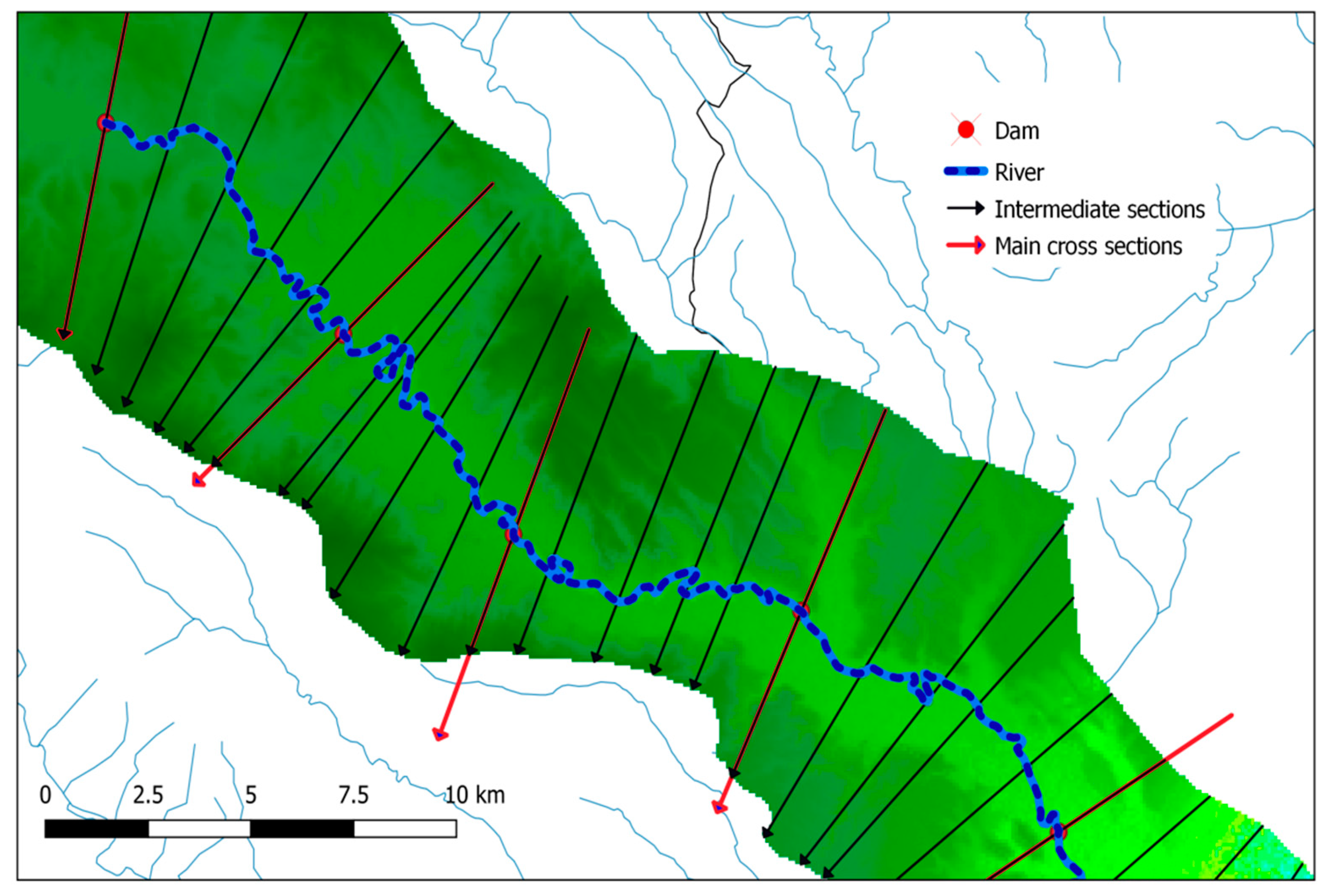
As mentioned above, the proposed flood propagation model only applies to a prismatic river reach. To account for this, an algorithm for the automatic generation of cross-sectional footprints has been implemented in order to divide the riverbed into several smaller prismatic branches. Given that a one-dimensional (1D) flood propagation model, like the one that is proposed in Section 2.2, requires a horizontal water level in the cross-section, the progressive cross sections should not overlap. The overlap would result in different water levels being evaluated for the same discharge at the point of intersection between the overlapped cross sections. Hence, the implemented algorithm creates fixed distance orthogonal cross-sectional footprints, whose inclinations are regularized by a cubic spline method, making the footprints independent of the riverbed shape. Once these main cross-sectional footprints are delineated, several intermediate sections are created in order to improve the model calculation step (see Figure 2). The rotational angle of these intermediate cross-sections is estimated on the basis of the interpolation between the two progressive main cross-sections.
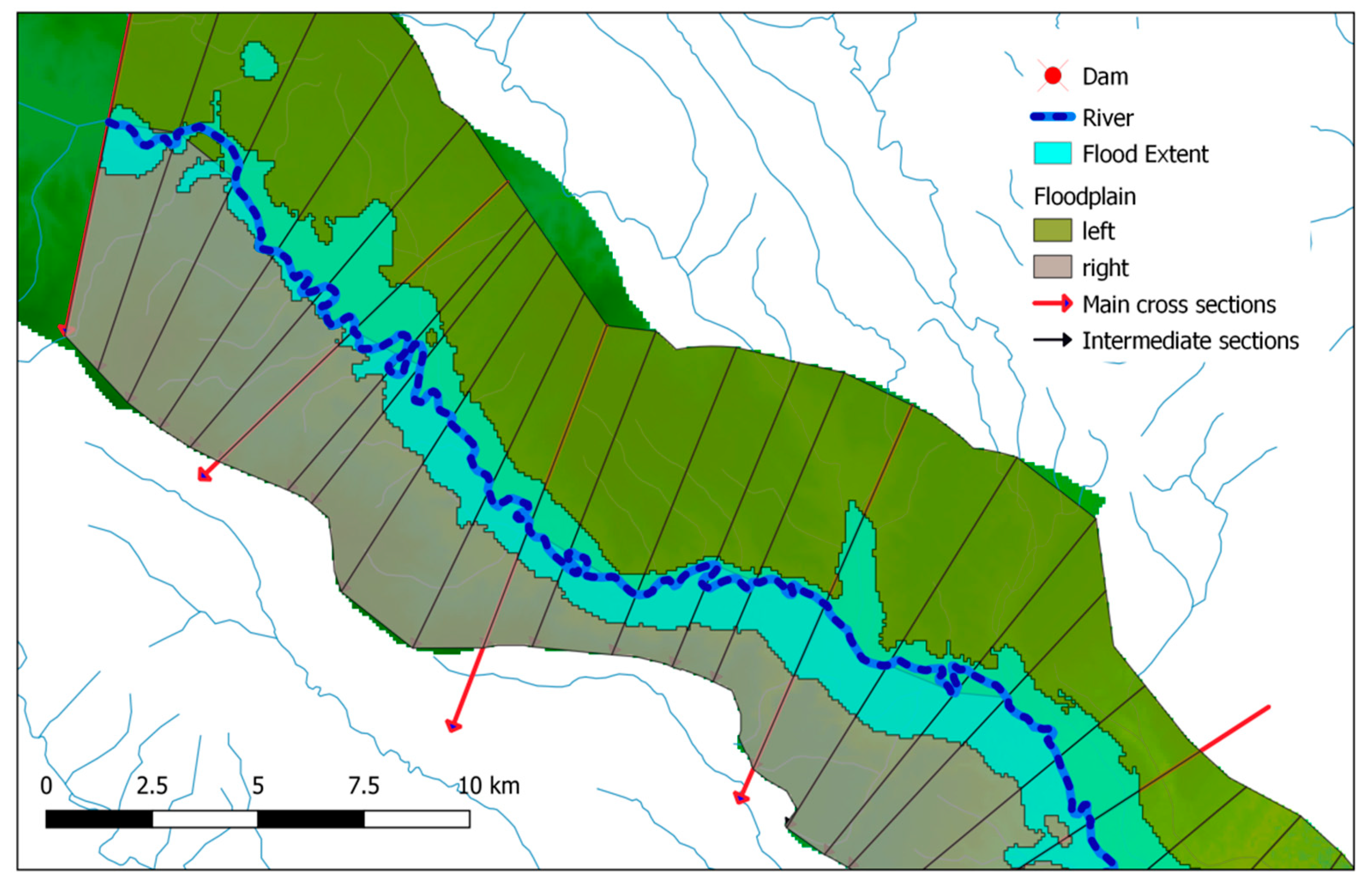
Once it is supplied with the river cross-sectional footprints, the algorithm can be employed to extract the river branch polygons (Figure 3). In addition, the elevation values are extracted from the DEM in order to assess the cross-sectional geometry.
In particular, the cross-sectional area, A, is evaluated with an iterative method that is based on varying the water depth, h, according to the following monomial formula:
The least squares method is applied in order to estimate the constant, and the exponent, , which best approximates the A value for Equation (9). On the basis of the estimated A value, the assigned Manning coefficient n, and the local slope i, a rating curve can be estimated for each cross section. The cross sections are much wider than the water depth, h, and, so, the cross section can be approximated as a rectangular shape, and the hydraulic radius, , (where, P is the wetted perimeter and L the width of the cross section), has a value that is near to the water depth (), when considering that . Thus, the discharge can be estimated as follows:
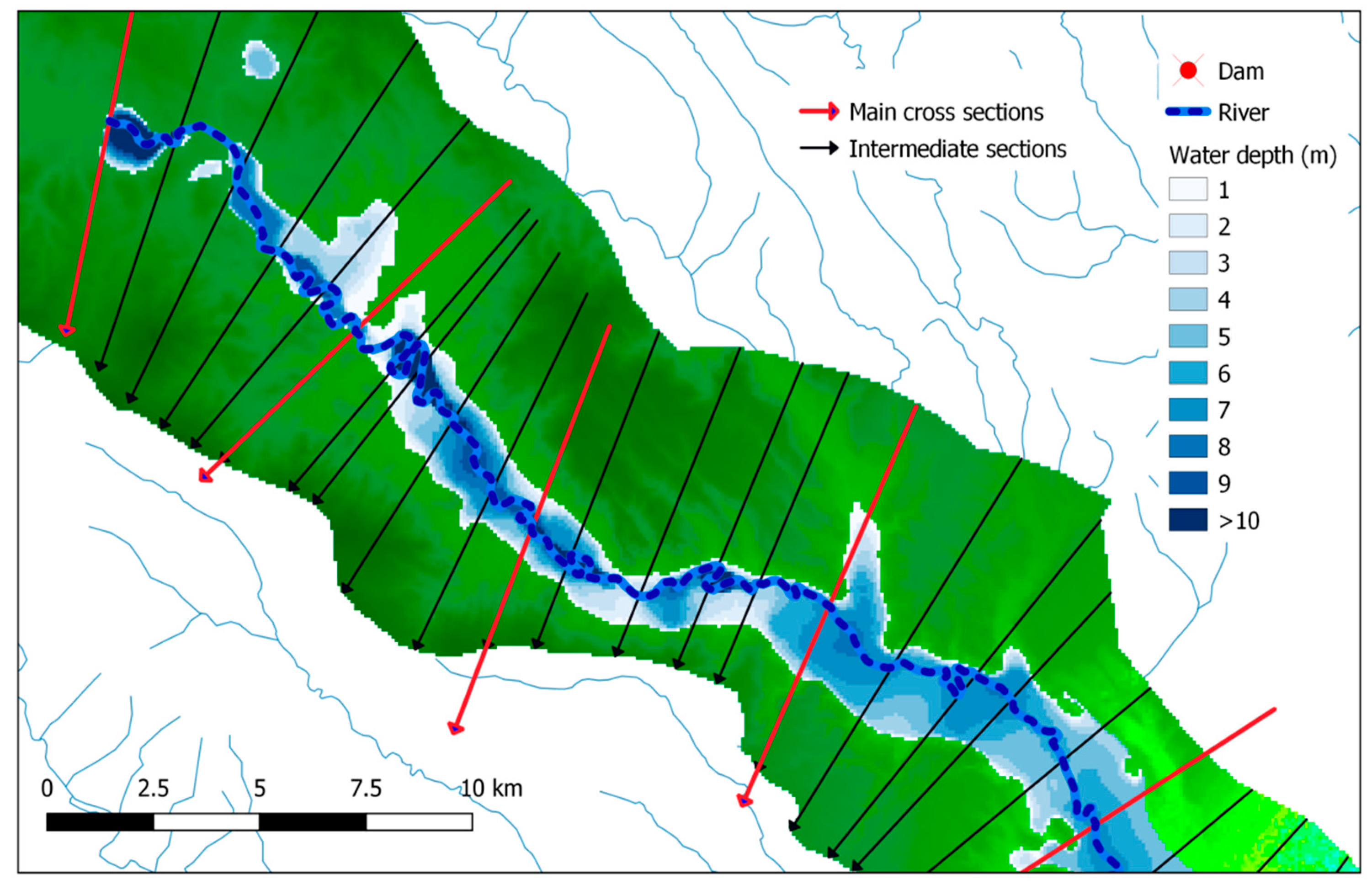
The rating curve formula in Equation (10) provides the information that is necessary to generate the water depth profile in each cross section. These results, coupled with the information that is extracted by the DEM elevation values, allow for the evaluation of the dam's valley flood hazard maps (see Figure 4).
2.4. The Implementation of the Tool: Libraries and Components
In this sub-section, the design and implementation of the proposed GIS tool are described. Particular focus is placed on the characteristics that may make it suitable for establishing a robust, modular, flexible, and repeatable approach for the mapping of dam-break flooded areas. The GIS tool’s conceptual design clearly follows an object-oriented implementation that deconstructs the calculation into a set of connectable pieces/components, which can then be assembled into applications of substantial complexity [30].
The tool is a cross-platform program, which is able to function across Windows, Linux, and Apple operating systems. The tool source code, as implemented in the Python programming language, is licensed under the GNU Public License (GPL) version 2 and it is shared through Github with a set of benchmark data and a brief user manual. Python has become one of the key languages used in GIS application development, which is, in part, due to its integration with the well-known GDAL/OGR (Geospatial Data Abstraction) library for raster and vector geospatial data formats [31]. Furthermore, the numeric extension, NumPy [32], allows for the efficient storage and manipulation of large amounts of numerical data, including GIS raster data, minimizing operational computation time.
The GIS tool structures are comprised of two main python scripts: (i) 'SanGiulianoDam_upload_data', which is made up of several methods that have the purpose of uploading input data into a geo-database; and, (ii) 'SanGiulianoDam_calc_dambrk', which contains the engine of the calculators. Users can easily and directly input these two scripts into QGIS [33] using the ScriptRunner plug-in [34]. Firstly, the user, running the 'SanGiulianoDam_upload_data' script, can create an SQLite Geodatabase [35] and upload the test data of the San Giuliano dam geometry and valley, provided by the authors, or, in the case that users have their own data (changing the input file path names), the user is able to upload the input of multiple case studies into the same Geodatabase in order to automatize the calculation of several dam-breaks. Subsequently, the calculation can be performed using the 'SanGiulianoDam_calc_dambrk' script. The resulting outputs have also been stored in the Geodatabase, e.g., the flood extent and water depth maps (divided in the river branch polygons), the flood propagation time, the maximum envelope of all the hydraulic parameters (see the ‘Q_H_MAX’ table in the geodatabase); however, the intermediate files will be stored in a file system folder with the same name as the user-provided dam unique identifier code (ID). In particular, the first method, i.e., 'SanGiulianoDam_upload_data', is composed using a method, called 'set_dam', which defines the dam for which the user would like to perform the dam-break analyses, by 'add_dam' that is used to import the dam geometry data, by 'add_StudyArea' that defines the study area downstream of the dam, by 'add_RiverPath' that reads the information of the vectorial layer of the river path downstream of the dam, by 'add_MainCrossSec' that is used to define the main river cross-section's footprint, and finally, by 'set_DTM', which is able to set the DEM to be used. As for the input files, the dam geometry is a point shapefile whose database contains six main attributes: 'DamID', i.e., the dam ID; 'Name', i.e., the dam name; 'DamType', i.e., the type of dam (G for gravity dam, V for arch dam); 'ResVolMcm', i.e., the reservoir total capacity in million cubic metres; 'Height_m', i.e., the hydraulic height in meters (the height to which the water rises behind the dam); and, 'BreachWidth', i.e., the average width of hypothetical breach into the dam. The river path input file is a linear shapefile that describes the main river in the dam valley. The river path should be digitalized by the user, starting from valley upstream. The cross-section profile should be added by the user in a linear shapefile digitalized from upstream. Moreover, each cross-section line should be composed of two points, i.e., the first one located on the left river bank and the second one on the right part of the bank. Finally, a polygon shapefile that defines the outline of the study area and a GeoTif raster file of the Digital Terrain Model (DTM) is needed for running the calculation(s). Indeed, the second script, i.e., 'SanGiulianoDam_calc_dambrk', contains five main methods that represent the calculator engine: 'Calc_IntermediatePoints' and 'Calc_IntermediateCrossSections' algorithms can delineate the intermediate river cross-section's footprint (see Figure 2); the 'Calc_ValleyGeometry' algorithm extracts the river branch polygons (see Figure 3) and the cross-sectional geometry through the elevation information of the DEM; 'DamBreakPropagation' runs the dam-break hydraulic analysis that is described in Section 2.2; and, 'CalcFloodArea' delineates the dam-break flood-prone areas, as described in Section 2.3.
2.5. Validation
The GIS tool results were analyzed and compared with historical data that are available by Pilotti et al. [36], which outline the outcomes of past studies that were performed by traditional hydrodynamic models (e.g., [36,37]) using a pixel to pixel comparison of the respective flood extent maps on two case studies (described in the next section), the San Giuliano potential dam-break and the 1923 Gleno dam-break. Using the flood maximum extent map, which was obtained by the traditional models or reconstructed by historical information, as a reference (i.e., gold standard truth), there were two ways in which the flooded area could be estimated using the GIS tool to be considered correct. To be considered as correct, the GIS tool must either correctly represent flooded or non-flooded pixels. To be considered incorrect, the GIS tool must erroneously either under- or over-predict the reference inundation extent [38]. As a result, a matrix, or contingency table, of four possible outcomes was produced. The outcomes are as follows: (i) the point was counted as a true positive if the GIS tool detected a flooded area when this condition was present in the flood map that was obtained by the traditional method, (ii) it was counted as a false negative if the GIS tool identified a point as non-flooded (negative), but this area was flooded in the reference inundation map, (iii) it was counted as a true negative if the site was defined as non-flooded by the flood extent map that was obtained by the reference inundation map and classified as negative using the GIS tool, (iv) finally, it was counted as a false positive if the GIS tool classified the area as flooded, but it was not flooded in the reference flood extent-map [13]. Figure 5 shows a schematic representation of the proposed contingency table. From this matrix, the true positive rate, or hit rate, was estimated as:
The false positive rate, or false alarm rate, was calculated as:
In addition to the contingency matrix analysis, additional statistical performance measurements, such as sensitivity, specificity, and accuracy, were performed. Sensitivity, or recall, refers to the proportion of correctly classified instants of flood pixels, whereas specificity evaluates the proportion of correctly classified instants of non-flood pixels. Accuracy refers to the proportion of pixels that are correctly classified. Sensitivity, specificity, and accuracy were calculated using [39]:
where, TP is true positive and defined as the total number of pixels predicted positive that are positive. FP is false positive and is equal to the number of pixels predicted positive that are negative. TN is true negative and equal to the number of pixels predicted negative that are negative. Finally, FN is false negative and equal to the number of pixels predicted negative that are positive.
3. Case Studies
The San Giuliano potential dam-break in a flat area in Basilicata (Figure 6) was analyzed by a comparison of the results of two approaches that are based on hydrodynamic models: (i) a past study proposed by Sole et al. [37], which was adopted by the Regional Authority for civil protection, where the numerical 1D model MIKE 11, as distributed by the Danish Hydraulic Institute, was used under unsteady conditions for the propagation of the dam-break water wave; and, (ii) a dam-break simulation, performed ad-hoc for this study, which considers recent advances in computational power and models and the availability of high-resolution topographic data, using a two-dimensional (2D) flood propagation model and a 10m resolution DEM. The study that was proposed by Sole et al. [37] and the traditional approach, performed by the authors, based on the 2D flood propagation model of [40] and high-resolution DEM, are briefly described in Section 3.1 to summarize the modelling experimental setup.
Moreover, the overall effectiveness and reliability of the proposed model were evaluated for the Gleno Dam, which is located in a steep area in the Central Italian Alps (see Figure 9 and Section 3.2), which suddenly collapsed due to structural deficiencies on the morning of December 1, 1923. Pilotti et al. [36] have reconstructed the Gleno dam-break event by recovering a great deal of historical information (i.e., old photographic images, reliable testimonies, and various written documents) made available online (see http://www.ing.unibs.it/~idraulica/gleno_testcase.htm), including both the quantitative historical delineation of a part (i.e., the first 2.3 kilometres downstream of the dam) of the dam-break flood extent map and the flood extent map simulated through a 1D hydrodynamic model. The results in Section 4 describe the outcome of the proposed method, in terms of flood extent area, in the above-mentioned case studies, and its comparison with the results of cited past studies through the validation strategies described in Section 2.5. Finally, a demonstrative application of the instantaneous dam-break due to structural failure, for 250 existing Italian masonry arch and gravity dams (Section 3.3), is briefly illustrated in order to testify the computational efficiency of such a tool for dam-break flood-mapping.
3.1. The San Giuliano Dam test case
The first application of the proposed GIS tool was carried out on a flat area in the Basilicata Region (Southern Italy), stretching for 56 km upstream of the mouth of the Bradano River (Figure 6). The surrounding land cover is mainly agricultural, being characterized by cereal and vegetable crops or orchards, while an extended area near the river mouth and along the coast is occupied by pinewoods. Moreover, several residential buildings and agricultural enterprises are located in the floodplains, with quite a few tourist resorts near the basin outlet along the coast. The mouth of the Bradano River is at high risk of flooding due to lithological and geomorphological properties [27]. This location is advantageous for human population development. Urban development occurred over time, along with the construction of several structural mitigation measures (i.e., levees, banks, artificial hills, and bridges), rendering the topography of the area extremely complex. During recent flood events [38], the greatest damages to agribusinesses, farms, and tourist complexes were recorded downstream from the San Giuliano dam. The latter plays a crucial role in the management of the water resources and irrigation for Basilicata and neighbouring regions. Moreover, the dam leads to a reduction of discharge in the case of a flood-wave, allowing for a diminished water depth.
In this context, we selected the San Giuliano dam as the first test case to perform a simulation with the proposed method and evaluate its performance, in terms of the extent of the flood map, through a comparison with the two traditional studies that are described in: (i) a past study proposed by Sole et al. [37] and adopted by the Regional Authority for civil protection aims, which is briefly described in Section 3.1.1; and, (ii) a dam-break simulation performed ad-hoc for this study considering, with respect to [37], the recent advancements in Computer Fluid Dynamic (CFD) techniques, but also the availability of high-resolution topographic data that is presented in Section 3.1.2. Table 1 summarizes the setup of the above-described modelling approach.
3.1.1. 1D Hydrodynamic Study
Sole et al. [37] used the commercial numerical 1D model MIKE 11, distributed by the Danish Hydraulic Institute, under unsteady conditions for the propagation of the dam-break water wave. The initial flood stage condition was a discharge of 1 m3/s. The hydrograph that is shown in Figure 7 was used as the upstream boundary condition. A constant hydrometric level in the river section that is closest to the sea was assumed as the downstream boundary condition. The cross-section was extracted using the available topographic map at either 1:5000 or 1:10000. In a few cases, elevation information, specifically 1:25000 topographic maps, from the Italian Military Geographical Institute (IGM), was used. The Manning roughness coefficient for the river channel and floodplain areas was assigned a value of 0.028 m-1/3 and it was assumed to be constant across all areas. This number corresponds to a non-maintained area with dense vegetation. Table 1 summarizes the setup of the modelling experiments.
3.1.2. 2D Hydrodynamic Modelling
A dam-break simulation, which was based on a 2D flood propagation model and a DEM at a 10m resolution, was performed. This method exploits many recent advancements in computational power and models and in the availability of high-resolution topographic data [41]. The 2D hydraulic model, called FLORA2D [40], was used for the flood propagation given that it was calibrated and applied with satisfactory results along the same river or in a similar environment [29,38,40].
However, when considering that the area immediately downstream from the San Giuliano dam revealed a steep canyon that could act as a barrier reflecting part of the discharge and increasing the water level higher than the maximum dam height, the use of the 2D models showed that water levels, which were produced by summing between the elevation at sea level and the water depth in a specific cell, were higher than the total estimated energy at the dam. Hence, in order to avoid this discrepancy in the conservation of energy equation at the base of the flood propagation models, the flood propagation model was used when considering the outflow hydrograph (shown in Figure 8) as the upstream boundary condition, as estimated using an iterative method based on 1D simulations, performed with the commercial software HEC-RAS [42], in a steady flow condition, assigning a boundary condition for which the maximum discharge in the canyon cannot be greater than the total estimated energy at the dam.
Moreover, critical water depth was applied as the downstream boundary condition and the null riverbed water level was set as the initial flood stage condition. Cross-sectional geometry was evaluated while using elevation information that was extracted from the freely-available DEM at a 5m resolution distributed by the RSDI Geoportal [43] of the Basilicata Region Authorities. Variable spatiotemporal Manning coefficients were used, as calibrated in Scarpino et al. [38], to take the dynamic effects of vegetation into account. Cell roughness varies with floodwater depth according to an empirical formula that depends on the type of vegetation [40]. In this application, the computational domain was defined by a square grid with a resolution of 10 m, while the time step was set to 2 seconds to ensure model stability (see Table 1 for a summary of the modelling experiments’ setup).
3.2. The Gleno Dam-Break Case Study
The Gleno Dam is a masonry arch gravity dam that is located in Valle del Povo, a small subcatchment of approximately 8.4 km2 in Valle di Scalve (174 km2), the main tributary valley of Valle Camonica (1460 km2) in Lombardy, Italy (as showed in Figure 9). In the early morning of December 1, 1923, about 40 days after the first complete reservoir filling, an 80 m long breach opened in the central portion of the Gleno Dam. The collapse was triggered by water seepage at the interface between the masonry base and the overlying structure. The effects of the flood propagation along the downstream river were catastrophic, resulting in 356 deaths and the destruction of three villages and five power stations, as well as a large number of isolated buildings and factories [36]. As a consequence of this catastrophic event, the multiple-arch design, which was in itself not responsible for the accident, was almost completely abandoned in Italy. Pilotti et al. [36] collected and analyzed detailed historical documentation compiled from several archives, in order to reconstruct the event. Furthermore, the authors simulated the event while using a numerical model. Pilotti et al. [36] described the dynamics of the reservoir emptying through a two-dimensional (2D) shallow water simulation and computed a one-dimensional (1D) simulation of the dam-break wave propagation along the downstream valley. All of the information about the model's input data, initial and boundary conditions, and the results, together with the part of the flood extent map that they reconstructed while using the collected historical information, have been published on the following website: http://www.ing.unibs.it/~idraulica/gleno_testcase.htm. Therefore, this information was used for validation purposes for the proposed GIS tool.
3.3. Example Application of Structural Failure for the 250 Existing Italian Masonry Arch and Gravity Dams
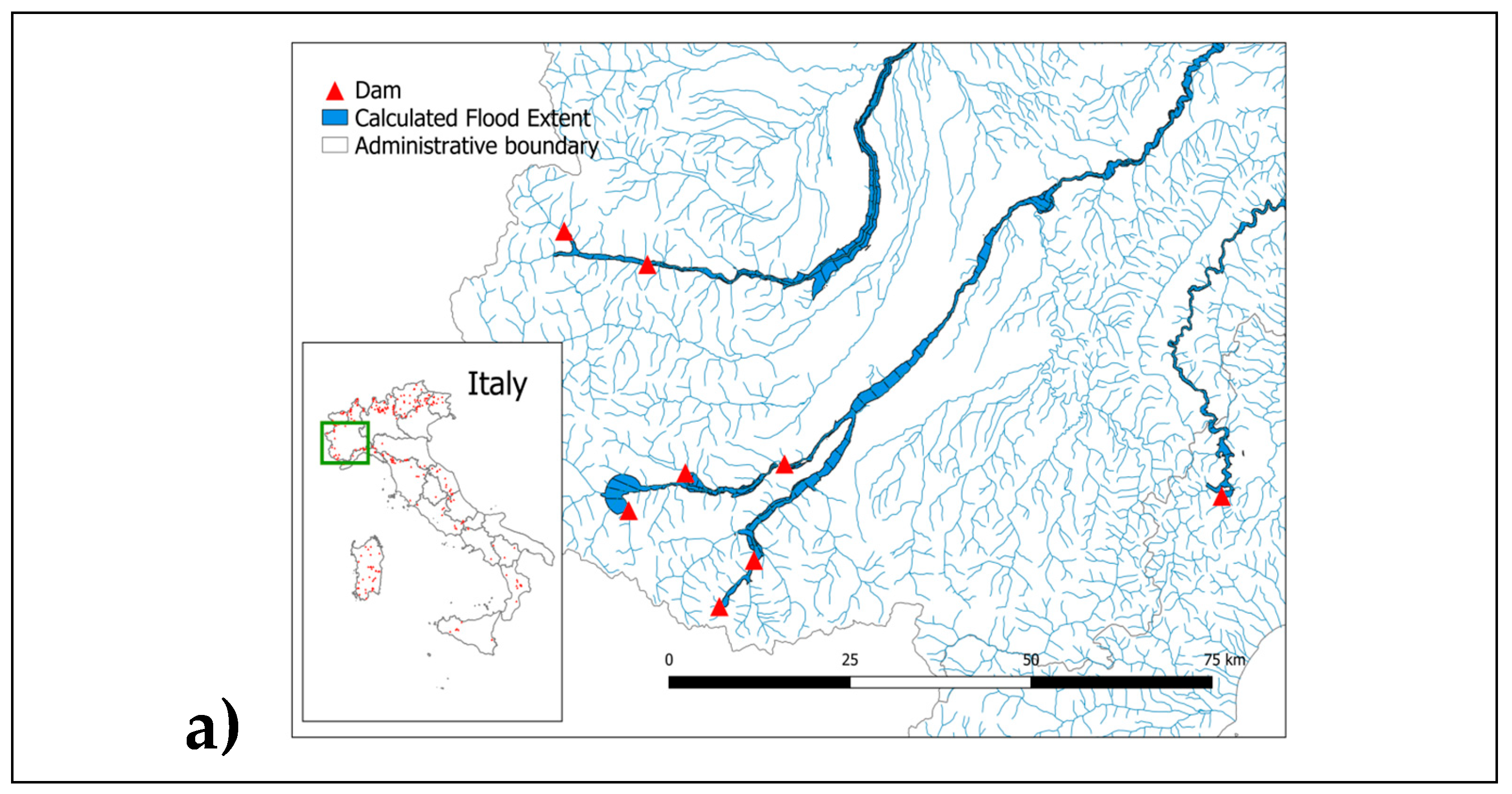
Using affordable and commonly available information, the GIS tool was used for mapping the hypothetical collapse of 250 Italian masonry dams. Figure 10 displays the location of the existing 250 Italian dams, for which the authors performed a rapid and inexpensive estimation of instantaneous dam-break (due to structural failure) that can be used, for example, by the authorities to support the prioritization of interventions or for further detailed analyses of traditional hydrodynamic simulations.
It should be noted that, it was assumed that propagation time would end when the peak discharge reached the value of the maximum natural peak with a return time of 500 years, following the ongoing Italian legislation guidelines, in cases where the flood wave of the dam-break propagation does not reach the sea or a large lake. The 500 years discharge value is estimated using the VAPI method ("Valutazione delle Piene in Italia"—"Evaluation of Flood Events in Italy"), commonly accepted in Italy, and developed by the "Gruppo Nazionale per la Difesa dalle Catastrofi Idrogeologiche"—"National Group of Hydrogeological Risks" (GNDCI) in the 1990s [44]. Section 4 describes the outcomes of the tool’s computational efficiency for a large number of dam-breaks.
4. Results
This section is devoted to the application and evaluation of the performance of the proposed model in different operating conditions, in terms of DTM resolution and the morphological context. The section also compares the proposed model with a set of hydrodynamic models with different setups (e.g., initial and boundary conditions).
Section 4.1 describes the application of the GIS tool to the instantaneous potential dam-break of the masonry San Giuliano dam in the south of Italy and its comparison with 1D and 2D hydrodynamic models. Moreover, Section 4.2 shows the validation of the proposed model using historical data of the 1923 Gleno dam-break provided by Pilotti et al. [36] as well as a comparison with a 1D hydrodynamic model that was proposed by Pilottie et al. [36] using the same input data. Finally, when considering the significant similarities with the reference maps obtained by historical data or by the hydrodynamic model, the tool is used in a demonstrative application on 250 existing Italian arch and gravity dams, using inexpensive and commonly available information. This application testifies its computational efficiency for an application of a large number of dam-breaks.
4.1. The Application on the San Giuliano Dam Case Study
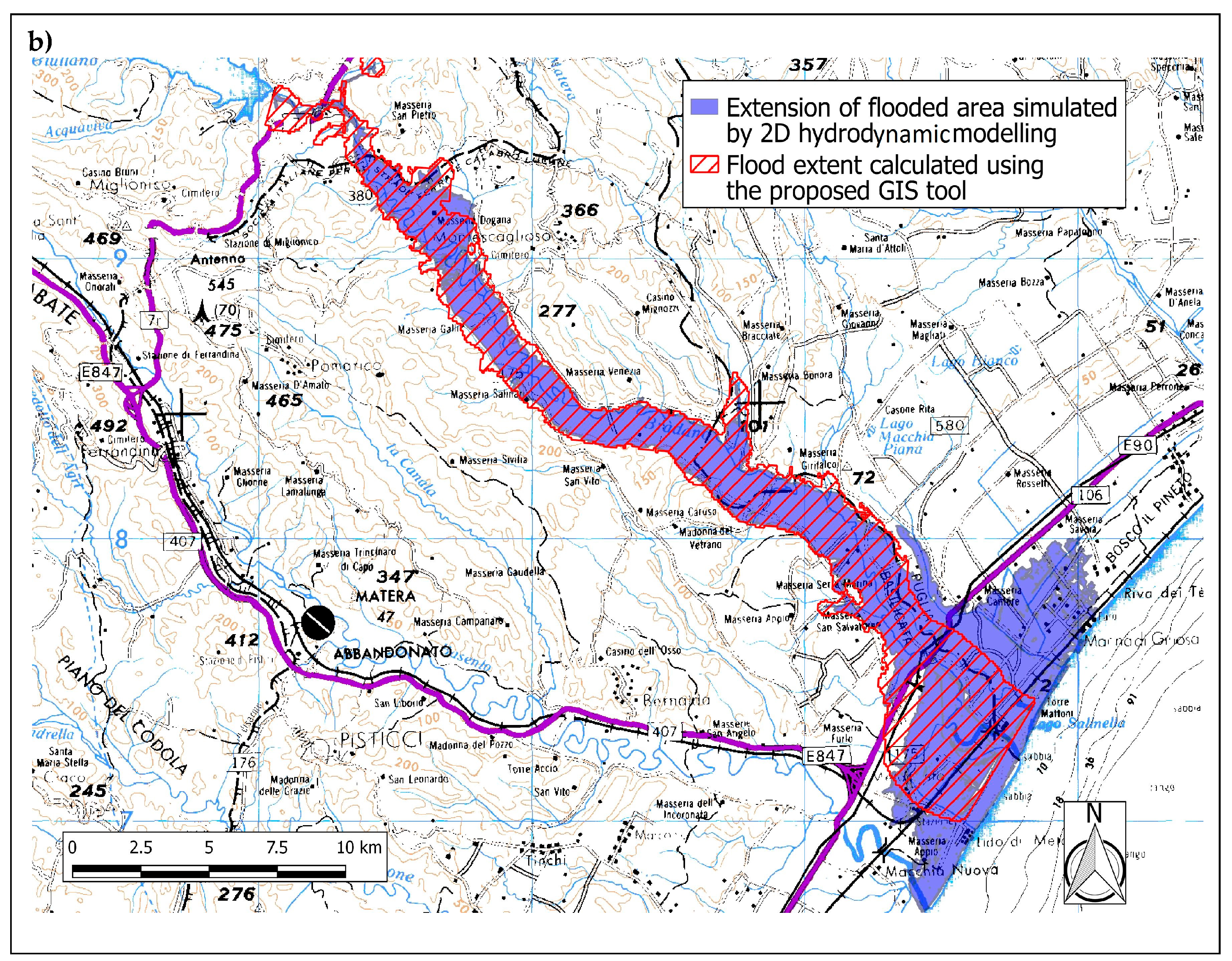
For the hypothetical San Giuliano dam-break, ground truth information was not readily available for the validation. Therefore, the tool outcomes were compared to the results of traditional studies based on 1D or 2D flood propagation models to test the accuracy and reliability of the model. Figure 11 shows the comparison of the flood extent estimated using our proposed approach and, respectively, (a) the extent of the flooded area that was simulated by Sole et al. [37], as described in Section 3.1.1, and (b) the the flood extent simulated by the authors through the 2D hydrodynamic model [40] that is described in Section 3.1.2. The qualitative results, as depicted in Figure 11 (a) and (b), show, in general, that the map calculated by the GIS tool and the results that were obtained by the hydrodynamic models are in accordance with each other. This is confirmed by the quantitative results, in terms of statistical performances, estimated as described in Section 2.5 and shown in Table 2.
The GIS tool hazard map resulted in a better agreement with the 2D hydraulic model [40] map with respect to the results of the study that was proposed by Sole et al. [37]. In particular, the specificity value of the 2D hydrodynamic model comparison was close to 90%, which confirmed that a consistent part of the map was considered to be flooded by both approaches, and a sensitivity value over 75% confirmed that several zones were correctly identified as non-flooded.
The GIS tool hazard map and 1D study outcome of Sole et al. [37] are in significant agreement, however to a lesser extent than the agreement that was found between the GIS tool output and the Flora2D map, as shown in Table 2. It is possible that this discrepancy was due to differences in the accuracy of elevation information available in the 1990s as compared to data that were extracted from the DEM. Changes in the landscape as a result of anthropogenic activity, including, for example, added infrastructure, buildings, and levees, may have also contributed to the noted discrepancy.
However, the GIS tool had a tendency to overestimate the extent of the flood map, immediately downstream of the dam (approximately the first 6 km), as obtained by these two traditional approaches. This is because the proposed GIS approach considered, in this case, the sum of the estimated water level and the kinetic depth in order to delineate the maximum extent of the propagated dam-break flood, which resulted in a condition of maximum safety for emergency or mitigation action planning. The GIS tool is designed as a rapid tool for the mapping of flood-prone areas and it can be used to complement, but not replace, results from hydrodynamic simulations. For this reason, the authors prefer to obtain and to show results, for this case study, for a condition of maximum safety delineating a flooded area that could be further refined by the use of detailed studies. The use of the GIS tool with a spatial uniform Manning coefficient equal to 0.06 m-1/3s for this application confirmed this idea. This value of the Manning coefficient, with respect to smaller values (such as the one used by Sole et al. [37]), results in a longer propagation time and a higher water depth, therefore resulting in a larger flooded area.
A condition of maximum safety is assured by maximizing the flooded area. It is important to note that Benoist [45] highlighted that a Manning coefficient value that is included in the range 0.066-0.028 m-1/3s is considerable for dam-break flood events. However, the extremely low value of the false positive rate, or false alarm rate, shows that the GIS tool’s overestimation of the rest of the valley, excluding the steep canyon, is quite low.
Moreover, in extremely flat zones closer to the river mouth, the 1D scheme that was adopted by Sole et al. [37] and the simplified 1D scheme proposed in the GIS tool are unable to adequately model the flood propagation when compared to the simulation that was performed with the 2D hydrodynamic method and high resolution DTM, confirming the outcomes of other past studies [29,46]. Indeed, the map on Figure 11 (b) demonstrated the successful adaptation of the GIS tool with respect to the 2D hydrodynamic approach's map in the upstream area, after the canyon, with a more marked topography, and a decrease in sensitivity performance in the flatter area, closer to the sea. This limitation of the GIS model could affect the evaluation of flood consequences when considering that populations and structures tend to be concentrated in the coastal areas or in zones that are close to a river delta.
The comparison outcomes demonstrated that the GIS tool provided good detection accuracies with simple data requirements, low costs, and reduced computational time. Indeed, the simulation using the GIS tool, which was carried out with a PC, Pentium Intel Core i5 Processor CPU 3.2 GHz, 8 GB RAM, only required 16s when compared to the 2D hydrodynamic modelling approach that required over five hours. This type of simplified approach is generally of great interest to researchers and decision-makers in a data scarce environment for flood mapping to complement the costly and timely traditional approaches, in terms of data collection and preparation.
4.2. Validation on the 1923 Gleno Dam-Break
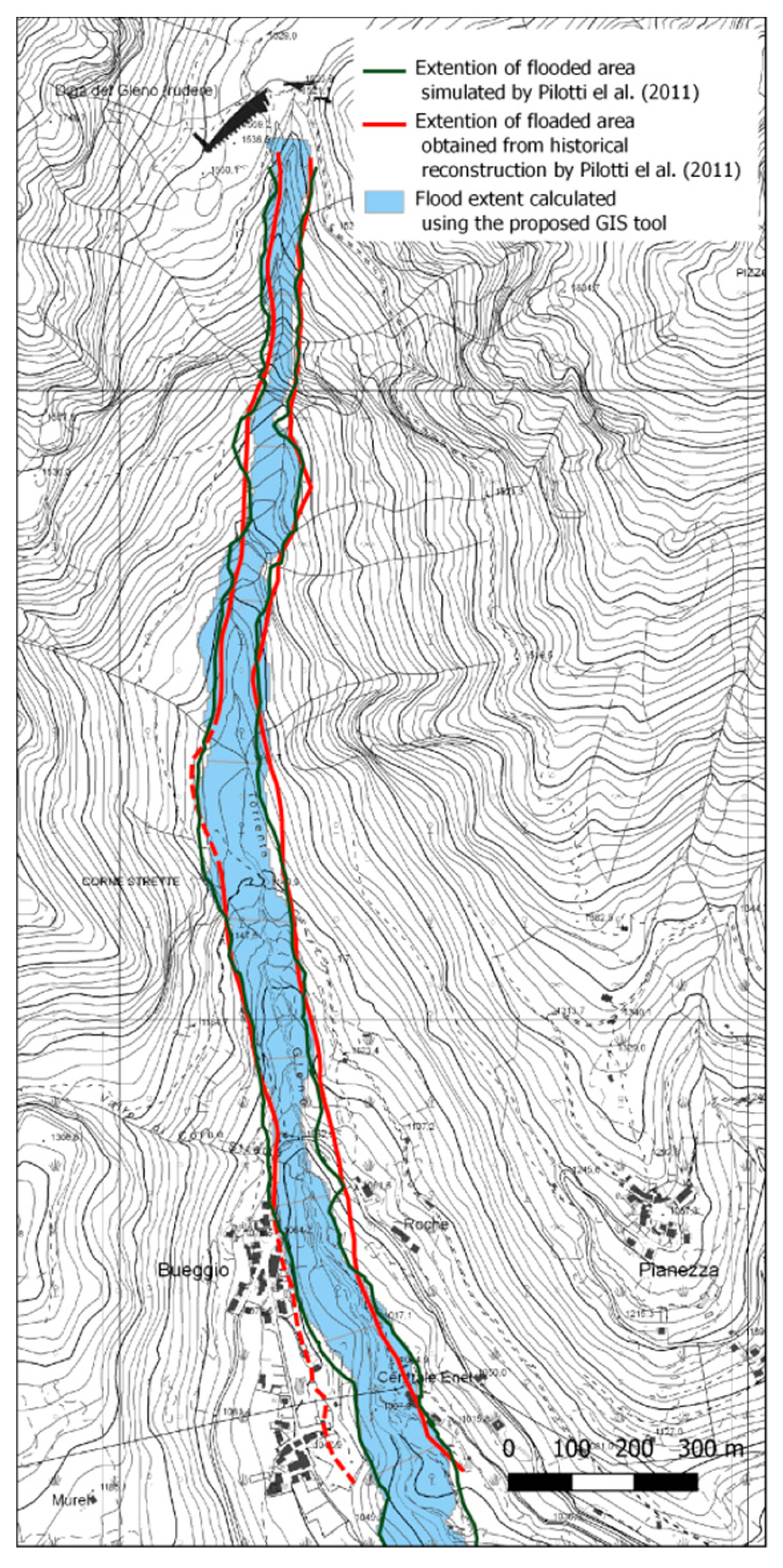
The overall effectiveness and reliability of the proposed model were evaluated for the 1923 Gleno dam-break, where Pilotti et al. provided historical information [36] that reconstructed the flood extent in the first 2.3 km immediately downstream of the dam. Moreover, the flood extent that was calculated by the GIS tool was compared with the result of a 1D numerical model that was performed by [36], as showed in Figure 12.
Using the dam geometry information and the DTM at 5m resolution, which are available at http://www.ing.unibs.it/~idraulica/gleno_testcase.htm, we obtained good performances, as shown in Table 3. The comparison with historical data results in a total accuracy of around 94% and a true positive rate, or hit rate, of 78.7%, demonstrating significant agreement in terms of the detection of flooded and non-flooded areas identified by the reference historical data. The GIS tool accuracy increases if compared with the 1D model that was proposed by Pilotti et al. [36], reaching a value of 96%.
It is important to highlight that we applied the GIS tool excluding the kinetic depth from the flood extent calculation when considering the availability of the historical information for this case study. However, the increased accuracy, with respect to the San Giuliano dam test case, could also be related to the high-resolution DTM that was used for the Gleno dam-break application and associated with the marked topography of the Gleno dam valley that made the 1D simplified scheme, as proposed in the GIS tool, more suitable for the estimation of flooded areas.
The good performance of the GIS tool with a different DTM resolution and morphological context (i.e., marked topography zones and flat areas) of the two above-discussed case studies, Gleno and San Giuliano dams, confirms its reliability and robustness under different operating conditions. Finally, it is important to note that we have shown the application of the tool with low resolution DTM at 90m for the San Giuliano test case to explore its application in data scarce environments when considering that high-resolution information on valley elevation is not often available, in particular, in developing countries.
4.3. Computational Performance on Large Number of Dam-Break Cases
The proposed rapid GIS tool, using affordable and commonly available information, allowed for the mapping of consequences for the hypothetical collapse of 250 Italian gravity dams. The computational efficiency of the GIS tool has been analyzed in such applications and the flood-prone areas map, for the 250 dam-breaks, required roughly 73 min. These analyses were carried out while using a PC, Pentium Intel Core i5 Processor 3.20 GHz, 8 GB RAM. The time that is required to construct the valley geometries is proportional to the number of DTM cells, independent of their size (i.e., pixel resolution). Instead, the time that is required to perform the calculation of the flood propagation is dependent on the number of river branch polygons (see Figure 3) obtained on the basis of the number of cross sections used. For this study case, the flood propagation calculation was approximately 9 min. Therefore, the computational time would be significantly reduced if several simulations on the same case study were performed.
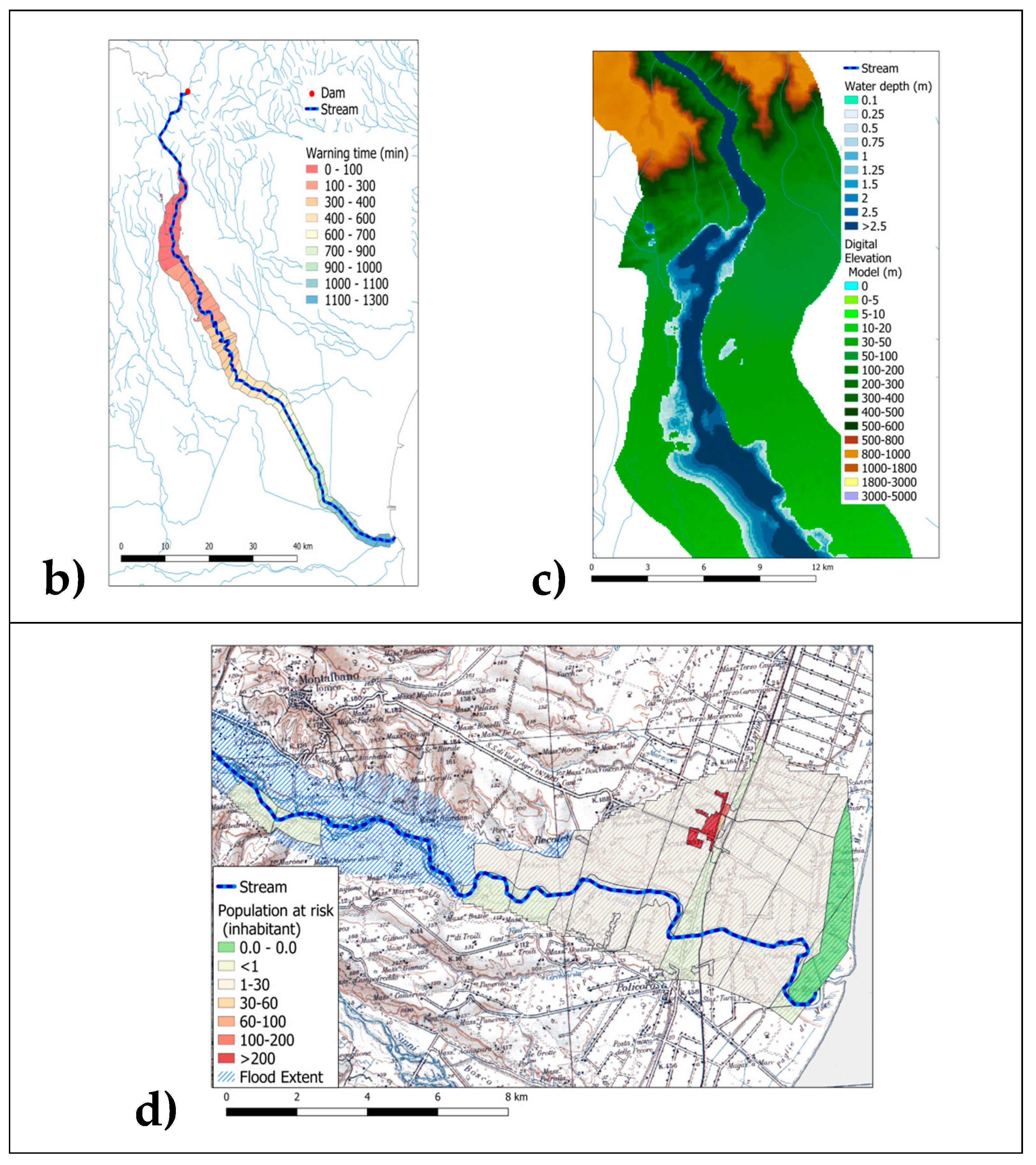
The tool resulted in an evaluation of the maximum flood extent map, the water depth map, the wave arrival time map, and population and structure damage maps (as shown in Figure 13). The damage maps were obtained through methodologies that were developed and implemented by the authors of the FloodRisk model of Albano et al. [30]. Figure 13 is an exemplification of the GIS tool’s demonstrative application. In particular, image (a) of Figure 13 shows an example of the flooded areas calculated for the potential failure of 250 dams, image (b) shows an example of the water depth map, and image (c) shows the wave arrival time maps for a dam in Northern Italy. Finally, image (d) presents the maps of population and structure damage for a dam in Southern Italy.
5. Discussion and Conclusion
This paper presented a cost-efficient geospatial tool that is capable of computing a map of areas that would be flooded in the event of a dam-break. The GIS tool can be applied on masonry (i.e., arch and gravity) dams for the analysis of an instantaneous dam-break due to structural failure. At present, the proposed tool is comprised of three calculation workflows that are capable of computing: (i) the evaluation of the instantaneous breach outflow discharge for masonry dams, (ii) the propagation of the flood in the downstream valley, and finally, (iii) the DEM-based delineation of flood-prone areas.
The main limitation of the tool is in regards to its application for dams that experience gradual failure, such as in the case of earthfill dams. This is because the hypotheses regarding front velocity and wave celerity (Section 2.1) that are employed in the proposed methodology cannot be applied to a decreasing discharge hydrograph. Therefore, the tool can be used for the estimation of the instantaneous failure of a masonry arch and gravity dams and it cannot be used for earthfill dams.
This topic must be studied in the future, as the study of earthfill dam-breaks requires addressing the important uncertainties related to branch dimensions, as discussed by several past studies [47,48,49,50,51,52]. The model can provide useful information, which complements but does not replace the results from hydrodynamic simulations, for risk delineation in data-scarce environments, and transboundary regions. Specifically, it can be employed towards a preliminary understanding of the hazard of dam-breaks to people and resources in the case of the realization of a new dam (e.g., for supporting the identification of the best site or the maximum dam volume). The model can support decision-makers, such as the Italian Dam Management Authority ('Servizio Dighe') or the owners of dam concessions, in the prioritization of interventions in the event that a large number of cases must be analyzed. Furthermore, it can support the Civil Protection Authority in the testing of several initial hypotheses during emergency situations, e.g., the modification of the initial water level/volume in the case of limited dam functionality or in the case of seismic risk. The GIS tools would be an appropriate alternative for probabilistic analyses with a large number of simulations that can be computationally lengthy. The proposed methodology was initially tested for the San Giuliano hypothetical dam-break and the results showed high accuracy and reliability in terms of the maximum flood extent map when compared to the traditional approaches. Moreover, the overall effectiveness and reliability of the proposed model were evaluated by comparing it with historical information and the results of a 1D numerical model, for the historical 1923 Gleno dam-break. Finally, the results of the GIS tool’s computational efficiency were tested on 250 existing Italian arch and gravity dams showing the potential of such a tool for a large number of masonry dam instantaneous failures. The results, which were carried out using a PC, Pentium Intel Core i5 Processor CPU 3.2 GHz, 8 GB RAM, required about 73 minutes of computationl time to construct the valley geometries, and the flood propagation calculation took roughly 9 minutes. Therefore, if several simulations on the same case study(s) were performed (e.g., in probabilistic modeling), the computational time would be substantially reduced.
Author Contributions
All authors contributed equally to this work.
Funding
This research received no external funding.
Acknowledgments
The work of the RSE author was financed by the Research Fund for the Italian Electrical System under a Contract Agreement between RSE S.p.A. and the Ministry of Economic Development - General Directorate for Nuclear Energy, Renewable Energy and Energy Efficiency in compliance with the Decree of March 8, 2006
Conflicts of Interest
The authors declare no conflict of interest.
References
- Fluixá-Sanmartín, J.; Altarejos-García, L.; Morales-Torres, A.; Escuder-Bueno, I. Review article: Climate change impacts on dam safety. Nat. Hazards Earth Syst. Sci. 2018, 18, 2471–2488. [Google Scholar] [CrossRef] [Green Version]
- Bonafè, A.; Mancusi, L.; Chieppa, V. The outlets vulnerability in the assessment of the safety of the dams/La vulnerabilità degli scarichi nella valutazione della sicurezza idraulica delle dighe. L’Acqua 2018, 6, 73–81. [Google Scholar]
- Falcucci, E.; Gori, S.; Bignami, C.; Pietrantonio, G.; Melini, D.; Moro, M.; Sarolli, M.; Galadini, F. The Campotosto Seismic Gap in Between the 2009 and 2016–2017 Seismic Sequences of Central Italy and the Role of Inherited Lithospheric Faults in Regional Seismotectonic Settings. Tectonics 2018, 37, 2425–2445. [Google Scholar] [CrossRef]
- De Moel, H.; Bouwer, L.M.; Aerts, J.C.J.H. Uncertainty and sensitivity of flood risk calculations for a dike ring in the south of the Netherlands. Sci. Total Environ. 2014, 473–474, 224–234. [Google Scholar] [CrossRef] [PubMed]
- Collenteur, R.A.; de Moel, H.; Jongman, B. The failed-levee effect: Do societies learn from flood disasters? Nat Hazards 2015, 76, 373. [Google Scholar] [CrossRef]
- Pu, J.H.; Shao, S.; Huang, Y.; Hussain, K. Evaluations of SWEs and SPH numerical modelling techniques for dam break flows. Eng. Appl. Comput. Fluid Mech. 2013, 7, 544–563. [Google Scholar]
- Lin, G.F.; Lai, J.S.; Guo, W.D. Performance of high-resolution TVD schemes for 1D dam-break simulations. J. Chin. Inst. Eng. 2005, 28, 771–782. [Google Scholar] [CrossRef]
- Manenti, E.; Pierobon, M.; Gallati, S.; Sibilla D’Alpaos, L.; Macchi, E.G.; Todeschini, S. Vajont Disaster: Smoothed Particle Hydrodynamics Modelling of the Postevent 2D Experiments. J. Hydraul. Eng. 2016, 142, 05015007. [Google Scholar] [CrossRef]
- Albano, R.; Mirauda, D.; Sole, A.; Adamowski, J. Modelling Large Floating Bodies in Urban Floods via a Smoothed Particle Hydrodynamics Model. J. Hydrol. 2016, 541 Pt A, 344–358. [Google Scholar] [CrossRef]
- George, A.C.; Nair, T.B. Dam Break analysis Using BOSS DAMBRK. Acquat. Procedia 2015, 4, 853–860. [Google Scholar] [CrossRef]
- Teng, J.; Jakeman, A.J.; Vaze, J.; Croke, B.F.W.; Dutta, D.; Kim, S. Flood inundation modelling: A review of methods, recent advances and uncertainty analysis. Environ. Model Softw. 2017, 90, 201–216. [Google Scholar] [CrossRef]
- Zhang, S.H.; Xia, Z.X.; Yuan, R.; Jiang, S.M. Parallel computation of a dam-break flow model using OpenMP on a multi-core computer. J. Hydrol. 2014, 512, 126–133. [Google Scholar] [CrossRef]
- Samela, C.; Albano, R.; Sole, A.; Manfreda, S. An open source GIS software tool for cost effective delineation of flood prone areas. Comput. Environ. Urban Syst. 2018, 70, 43–52. [Google Scholar] [CrossRef]
- Albano, R.; Craciun, I.; Mancusi, L.; Sole, A.; Ozunu, A. Flood damage assessment and uncertainity analysis: The case study of 2006 flood in Ilisua Basin in Romania. Carpath. J. Earth Environ. Sci. 2017, 12, 335–346. [Google Scholar]
- Seyedashraf, O.; Rezaei, A.; Akhtari, A.A. Dam break flow solution using artificial neural network. Ocean Eng. 2017, 142, 125–132. [Google Scholar] [CrossRef]
- Seyedashraf, O.; Mehrabi, M.; Akhtari, A.A. Novel approach for dam break flow modelling using computational intelligence. J. Hydrol. 2018, 559, 1028–1038. [Google Scholar] [CrossRef]
- Albano, R.; Mancusi, L.; Sole, A.; Adamowski, J. Sustainable and collaborative strategies for EU flood risk management: FOSS and Geospatial Tools—Challenge and opportunities for operative risk analysis. ISPRS Int. J. Geo-Inf. 2015, 4, 2704–2727. [Google Scholar] [CrossRef]
- Ritter, A. Die Fortpflanzung der Wasserwelle (Generation of the water wave). Z. Ver. Dtsch. Ing. 1982, 36, 947–954. (In German) [Google Scholar]
- Ven Te Chow. Open-Channel Hydraulics; McGraw-Hill Companies: New York, NY, USA, 1959. [Google Scholar]
- CGIAR-CSI Shuttle Radar Topography Mission DEM. Available online: http://srtm.csi.cgiar.org/ (accessed on 10 April 2017).
- Registro Italiano Dighe. Available online: www.registroitalianodighe.it (accessed on 10 July 2015).
- ANIDEL. Le dighe di ritenuta degli impianti idroelettrici italiani—Tecnica delle dighe di ritenuta in Italia; Associazione Nazionale Imprese Produttrici e Distributrici di Energia Elettrica: Roma, Italy, 1961. [Google Scholar]
- ENEL. Dighe di ritenuta degli impianti idroelettrici italiani, Le dighe appartenenti all’ENEL di costruzione posteriore al 1953; ENEL: Roma, Italy, 1970. [Google Scholar]
- Geoportale Nazionale—Ministero dell’Ambiente e della Tutela del Territorio e del Mare (Italia). Available online: http://www.pcn.minambiente.it/mattm/ (accessed on 10 March 2018).
- PostGIS—Spatial and Geographic objects for PostgreSQL. Available online: https://postgis.net/ (accessed on 20 April 2018).
- Marchi, E.; Rubatta, A. Meccanica dei Fluidi; UTET: Torino, Italy, 1981. [Google Scholar]
- Hunt, B. A perturbation solution of the flood-routing problem. J. Hydraul. Res. 1987, 25, 215–234. [Google Scholar] [CrossRef]
- Molinaro, P.; Fenaroli, G. Discussione dell’articolo di Hunt B. J. Hydraul. Res. 1988, 3, 26. [Google Scholar]
- Albano, R.; Sole, A.; Adamowski, J.; Perrone, A.; Inam, A. Using FloodRisk GIS freeware for uncertainty analysis of direct economic flood damages in Italy. Int. J. Appl. Earth Obs. Geoinf. 2018, 73, 220–229. [Google Scholar] [CrossRef]
- Albano, R.; Mancusi, L.; Sole, A.; Adamowski, J. FloodRisk: A collaborative, free and open-source software for flood risk analysis. Geomat. Nat. Hazards Risk 2017, 8, 1812–1832. [Google Scholar] [CrossRef]
- GDAL/OGR (Geospatial Data Abstraction) Python Library. Available online: https://www.gdal.org/ (accessed on 15 January 2018).
- NumPy Python Library. Available online: http://www.numpy.org/ (accessed on 7 May 2019).
- QGIS Desktop GIS. Available online: https://www.qgis.org/it/site/ (accessed on 7 May 2019).
- ScriptRunner QGIS Plugin. Available online: Github.com/g-sherman/Script-Runner (accessed on 7 May 2019).
- SQLite Database. Available online: https://www.sqlite.org/index.html (accessed on 7 May 2019).
- Pilotti, M.; Maranzoni, A.; Tomirotti, M.; Valerio, G. 1923 Gleno Dam Break: Case Study and Numerical Modelling. J. Hydraul. Eng. 2011, 137, 480–492. [Google Scholar] [CrossRef]
- Sole, A.; Crisci, A.; Scuccimarra, V. Studio dell’onda di sommersione conseguente all’ipotetico collasso e a manovre agli organi di scarico della diga si S. Giuliano; Pubblicazione interna DIFA Unibas: Potenza, Italy, 1997. [Google Scholar]
- Scarpino, S.; Albano, R.; Cantisani, A.; Mancusi, L.; Sole, A.; Milillo, G. Multitemporal SAR Data and 2D Hydrodynamic Model Flood Scenario Dynamics Assessment. ISPRS Int. J. Geo-Inf. 2018, 7, 105. [Google Scholar] [CrossRef]
- Chapi, K.; Singh, V.P.; Shrizadi, A.; Shahabi, H.; Bui, D.T.; Pham, B.T.; Khorsravi, K. A novel hybrid artificial intelligence approach for flood susceptibility assessment. Environ. Model. Softw. 2017, 95, 229–245. [Google Scholar] [CrossRef]
- Cantisani, A.; Giosa, L.; Mancusi, L.; Sole, A. FLORA-2D: A New Model to Simulate the Inundation in Areas Covered by Flexible and Rigid Vegetation. Int. J. Eng. Innov. Technol. 2014, 3, 179–186. [Google Scholar]
- Sole, A.; Giosa, L.; Albano, R.; Cantisani, A. The laser scan data as a key element in the hydraulic flood modelling in urban areas. In Proceedings of the International Archives of the Photogrammetry, Remote Sensing and Spatial Information Sciences—ISPRS Archive, London, UK, 29–31 May 2013. [Google Scholar]
- HEC-RAS—Hydrologic Engineering Center. Available online: https://www.hec.usace.army.mil/software/hec-ras/ (accessed on 15 June 2017).
- RSDI—Geoportale Basilicata—Regione Basilicata. Available online: https://rsdi.regione.basilicata.it/ (accessed on 30 August 2018).
- GNDCI—Progetto VAPI. Available online: http://www.gndci.cnr.it/it/vapi/welcome_it.htm (accessed on 20 August 2018).
- Benoist, G. Les études d’ondes de submersion des grands barrages d’EDF. La Houille Blanche 1989, 1, 43–54. (In French) [Google Scholar] [CrossRef]
- Tsakiris, G. Flood risk assessment: Concepts, modelling, applications. Nat. Hazards Earth Syst. Sci. 2014, 14, 1361–1369. [Google Scholar] [CrossRef]
- Tsai, C.W.; Yeh, J.-J.; Huang, C.-H. Development of probabilistic inundation mapping for dam failure induced floods. Stoch. Environ. Res. Risk Assess. 2019, 33, 91–110. [Google Scholar] [CrossRef]
- Peter, S.J.; Siviglia, A.; Nagel, J.; Marelli, S.; Boes, R.M.; Vetsch, D.; Sudret, B. Development of Probabilistic Dam Breach Model Using Bayesian Inference. Water Resour. Res. 2018, 54, 4376–4400. [Google Scholar] [CrossRef] [Green Version]
- Wahl, T.L. Uncertainty of predictions of embankment dam breach parameters. J. Hydraul. Eng. 2004, 130, 389–397. [Google Scholar] [CrossRef]
- Froehlich, D.C. Embankment dam breach parameters and their uncertainties. J. Hydraul. Eng. 2008, 134, 1708–1721. [Google Scholar] [CrossRef]
- Ahmadisharaf, E.; Kalyanapu, A.J.; Thames, B.A.; Lillywhite, J. A probabilistic framework for comparison of dam breach parameters and outflow hydrograph generated by different empirical prediction methods. Environ. Model. Softw. 2016, 86, 248–263. [Google Scholar] [CrossRef] [Green Version]
- Ahmadisharaf, E.; Bhuyian, M.-N.M.; Kalyanapu, A.J. Impact of spatial resolution on downstream flood hazard due to dam break events using probabilistic flood modelling. In Proceedings of the 5th Dam Safety Conference, Providence, RI, USA, 16–20 September 2012; pp. 263–276. [Google Scholar]
Figure 1.
Predicted San Giuliano dam-break outflow hydrograph.

Figure 2.
Example of the cross-sectional footprint delineation for an area of the valley downstream from the San Giuliano dam.
Figure 2.
Example of the cross-sectional footprint delineation for an area of the valley downstream from the San Giuliano dam.

Figure 3.
Example of the flood extent maps for an area of the valley downstream from the San Giuliano dam.
Figure 3.
Example of the flood extent maps for an area of the valley downstream from the San Giuliano dam.

Figure 4.
Example of the flood water depth maps for an area of the valley downstream from the San Giuliano dam.
Figure 4.
Example of the flood water depth maps for an area of the valley downstream from the San Giuliano dam.

Figure 5.
Schematic representation of the contingency table adopted to test the performance of the Geographic Information System (GIS)-tool in terms of dam-break flood extent map.
Figure 5.
Schematic representation of the contingency table adopted to test the performance of the Geographic Information System (GIS)-tool in terms of dam-break flood extent map.

Figure 6.
The San Giuliano Dam valley case study.

Figure 7.
San Giuliano dam-break outflow hydrograph according to the methods of Sole et al. (1997). Source: [37].
Figure 7.
San Giuliano dam-break outflow hydrograph according to the methods of Sole et al. (1997). Source: [37].

Figure 8.
San Giuliano dam-break outflow hydrograph according to the approach that used the 2D propagation model of [40].
Figure 8.
San Giuliano dam-break outflow hydrograph according to the approach that used the 2D propagation model of [40].

Figure 9.
The Gleno dam case study.

Figure 10.
Overall representation of the location of the 250 Italian dams analyzed in this study.

Figure 11.
(a) Comparison of the flooded area estimated by the proposed GIS tool for the San Giuliano potential dam-break with the flooded area calculated by Sole et al., 1997 [33]; (b) Comparison of the flooded area estimated by the proposed GIS tool for the San Giuliano potential dam-break with the flooded area calculated by the 2D hydrodynamic model proposed by Cantisani et al., 2013 [40].


Figure 12.
Comparison of the flooded area estimated by the proposed GIS tool for the first 2.3 km of the Gleno Dam-break with the flooded area (i) simulated by the hydrodynamic model and (ii) obtained from historical reconstruction both by Pilotti at al. [36].
Figure 12.
Comparison of the flooded area estimated by the proposed GIS tool for the first 2.3 km of the Gleno Dam-break with the flooded area (i) simulated by the hydrodynamic model and (ii) obtained from historical reconstruction both by Pilotti at al. [36].

Figure 13.
GIS tool example application of instantaneous dam-break due to structural failure for the 250 existing Italian mansory arch and gravity dams: (a) an example of the flooded areas calculated for the potential failure of 250 dams; (b) an example of the water depth map for a dam area in Northern Italy; (c) an example of the wave arrival time map of a dam in Northern Italy; and, (d) an example of a loss of life map for an area of a dam in Southern Italy.


Table 1.
Summary of the numerical modelling setup for the San Giuliano case study by Sole et al. [37], by the two-dimensional (2D) numerical model of Cantisani et al. [40] and by the proposed GIS tool.
| Method | Spatial Resolution | Initial Conditions | Upstream Boundary Condition | Downstream Boundary Condition | Manning's Coefficient |
|---|---|---|---|---|---|
| The proposed GIS tool | 0.5 cross section per km | Dry | Dam-break outflow hydrograph of fig. 1 | None | 0.06 m-1/3s |
| Sole et al. [37] | 1 cross section per km | Discharge of 1 m3/s | Dam-break outflow hydrograph of fig. 7 | Sea level | 0.028 m-1/3s |
| 2D hydrodynamic modelling | 10 m DEM | Dry | Dam-break outflow hydrograph of fig. 8 | Critical water depth | Spatial variation |
Table 2.
Results of the GIS tool performance compared, respectively, with the 2D propagation model approach and with respect to Sole et al., 1997 in terms of a flood extent map for the San Giuliano case study: false positive rate rfp, true positive rate rtp, false negative rate rfn, and accuracy, sensitivity, and specificity.
| rfp | rtp | Accuracy | Sensitivity | Specificity | |
|---|---|---|---|---|---|
| 2D propagation model [40] | 10.1 | 78.5 | 86.5 | 75.5 | 89.9 |
| Sole et al. [37] | 19.9 | 59.7 | 74.2 | 57.7 | 80.1 |
Table 3.
Results of the GIS tool performance in terms of the flooded area compared respectively with the results simulated by the hydrodynamic model of Pilotti et al. [36] and obtained from historical reconstruction by Pilotti et al. [36] for the Gleno dam-break case study.
| rfp | rtp | Accuracy | Sensitivity | Specificity | |
|---|---|---|---|---|---|
| Historical reconstruction of flooded area | 2.2 | 78.7 | 94.8 | 78.7 | 97.9 |
| Flooded area simulated by hydrodynamic model | 1.5 | 86.9 | 96.8 | 86.9 | 98.5 |
© 2019 by the authors. Licensee MDPI, Basel, Switzerland. This article is an open access article distributed under the terms and conditions of the Creative Commons Attribution (CC BY) license (http://creativecommons.org/licenses/by/4.0/).
Share and Cite
MDPI and ACS Style
Albano, R.; Mancusi, L.; Adamowski, J.; Cantisani, A.; Sole, A. A GIS Tool for Mapping Dam-Break Flood Hazards in Italy. ISPRS Int. J. Geo-Inf. 2019, 8, 250. https://0-doi-org.brum.beds.ac.uk/10.3390/ijgi8060250
AMA Style
Albano R, Mancusi L, Adamowski J, Cantisani A, Sole A. A GIS Tool for Mapping Dam-Break Flood Hazards in Italy. ISPRS International Journal of Geo-Information. 2019; 8(6):250. https://0-doi-org.brum.beds.ac.uk/10.3390/ijgi8060250
Chicago/Turabian StyleAlbano, Raffaele, Leonardo Mancusi, Jan Adamowski, Andrea Cantisani, and Aurelia Sole. 2019. "A GIS Tool for Mapping Dam-Break Flood Hazards in Italy" ISPRS International Journal of Geo-Information 8, no. 6: 250. https://0-doi-org.brum.beds.ac.uk/10.3390/ijgi8060250
Note that from the first issue of 2016, this journal uses article numbers instead of page numbers. See further details here.