Article

Spatial Keyword Query of Region-Of-Interest Based on the Distributed Representation of Point-Of-Interest

College of Electronic Science and Technology, National University of Defense Technology, Changsha 410073, China
*
Author to whom correspondence should be addressed.
ISPRS Int. J. Geo-Inf. 2019, 8(6), 287; https://0-doi-org.brum.beds.ac.uk/10.3390/ijgi8060287
Submission received: 21 April 2019 / Revised: 18 June 2019 / Accepted: 19 June 2019 / Published: 20 June 2019

Abstract

:
The tremendous advance in information technology has promoted the rapid development of location-based services (LBSs), which play an indispensable role in people’s daily lives. Compared with a traditional LBS based on Point-Of-Interest (POI), which is an isolated location point, an increasing number of demands have concentrated on Region-Of-Interest (ROI) exploration, i.e., geographic regions that contain many POIs and express rich environmental information. The intention behind the POI is to search the geographical regions related to the user’s requirements, which contain some spatial objects, such as POIs and have certain environmental characteristics. In order to achieve effective ROI exploration, we propose an ROI top-k keyword query method that considers the environmental information of the regions. Specifically, the Word2Vec model has been introduced to achieve the distributed representation of POIs and capture their environmental semantics, which are then leveraged to describe the environmental characteristic information of the candidate ROI. Given a keyword query, different query patterns are designed to measure the similarities between the query keyword and the candidate ROIs to find the k candidate ROIs that are most relevant to the query. In the verification step, an evaluation criterion has been developed to test the effectiveness of the distributed representations of POIs. Finally, after generating the POI vectors in high quality, we validated the performance of the proposed ROI top-k query on a large-scale real-life dataset where the experimental results demonstrated the effectiveness of our proposals.

1. Introduction

Recent years have witnessed the rapid development of Internet technologies and sensor devices, which, in turn, has resulted in the explosive growth of geo-related information. According to the statistics, 18.78% of web resources contain geographic location information and 18.6% of information retrieval is related to location [1]. The current research focus is spatiotemporal data mining and pattern discovery via multi-source geospatial big data. The corresponding achievements are widely used in urban computing, social analysis, environmental monitoring, and other fields, which greatly improve the quality of people’s life [2,3]. As an important research direction, location-based services (LBSs) have attracted great attention from both the academic and industrial communities. A valuable research problem in this field is exploring the locations of interest in the city by mining geo-tagged data. However, most of the current location services only concentrate on the search of isolated locations, such as Point-Of-Interest (POI) queries and ignore the user’s demand for Region-Of-Interest (ROI) exploration. In many real-life application scenarios, it is common for users to find multi-functional ROIs related to their requests, e.g., a person is hoping to watch a movie in a nearby cinema after drinking coffee in a cafe, which is a difficult question for traditional POI based methods to answer. In addition, research on ROI exploration can not only create a better service in application, but also create high research value in urban function analysis. It is worth noting that we used the definition of geographic regions [4] rather than image areas [5] for the ROI in our article.
At present, the existing ROI exploration methods are mainly based on the statistical information or the density information of the query elements [6,7,8,9], such as POIs with certain keywords [10,11], while neglecting the influence of internal and environmental characteristics of the region. Theoretically, judging how much the ROI is related to a query should take into consideration the distribution and type characteristics of all geographic objects in the ROI. For instance, the regional ecology decides the association between the ROI and query requirements. However, it is still quite challenging to measure the relevance between each spatial object and the query requirements [12]. Moreover, spatial-keyword queries with multiple query elements still remain difficult to cope with [11], and they are usually more complex and result in a high time consumption.
Bao J et al. [13] revealed that there was a strong correlation between the spatial distribution of geographic objects and their categories, indicating that spatial objects could be classified by their neighbors. Consequently, inspired by [14], we utilized a distributed representation model, i.e., the Word2Vec model, to explore the spatial distribution characteristics of geographic objects and the relatedness between their types. Specifically, this model projects words into a distributed space in accordance with its context in the document to capture the spatial distribution features and environmental information of each type of spatial object, such as the POI. Thus, the spatial object can be transferred into a high-dimensional vector, which encodes the association characteristics between the POI types. Then, in order to achieve an efficient query of the relevant ROI, we executed a grid division on the whole research region so that each grid contained a certain number of POIs. With the grids viewed as the candidate ROIs, the ROI vectors were obtained by their internal POI vectors, which implies the type characteristics and spatial distribution of each candidate ROI. Finally, after designing different query patterns, the similarity score between each ROI vector and the vectorized query conditions was calculated to find the top-K ROIs related to the query.
The contributions can be summarized as follows:
  • Unlike traditional ROI exploration based on the statistical information of query elements, we studied ROI exploration for environmental semantics and distribution characteristics, which introduced new opportunities and challenges. We were the first to utilize the spatial distribution and the semantic information of the POI in ROI exploration.
  • We proposed a novel POI corpus construction method and used Word2Vec model to acquire the distributed semantic representation of the POI. An evaluation metric was developed to measure whether our proposed method could effectively capture the environmental semantics and type characteristics of the POI, and also prove the association between POI spatial distribution and their types.
  • The grid division was constructed to realize the distributed representation of the regional feature information of the candidate ROI. After the calculation method of the similarity score between the ROI vector and query condition was designed to achieve the top-K query of the keyword-based ROI, we verified that the proposed method achieved significant improvements over the baselines in a large-scale real dataset.
  • Considering the extension of the ROI multi-keyword query mode, we demonstrated the validity and feasibility of the multi-keyword query.
The rest of this paper is organized as follows. Section 2 overviews the related work. Section 3 formally defines the statement of our problem. Our method is elaborated in Section 4. Section 5 proves the efficiency of the POI vectors and evaluates the performance of the proposed method by comparison. Finally, we briefly conclude the paper in Section 6.

2. Related Works

Spatial keyword search, which is a fully developed research field in geographic information retrieval, has achieved valuable and significant research results [10,15,16,17]. The related research methods can be mainly divided into spatial-first approaches and keyword-first approaches [18]. While the spatial-first approaches usually perform geographic queries on spatial indexes to obtain the target objects [19], the keyword-first approaches are more relevant to our work, where existing research has focused on the textual association between the target geographic object and the query description to find relevant locations (such as POI) [20,21]. Unlike the traditional POI-based query methods above-mentioned, our study emphasized the ROI exploration related to the spatial keyword query. There have been some studies on ROI search in recent years, which can be roughly divided into two different research methods: a search based on density and a search based on fixed division. The former attempts to explore the density of the POIs related to the query keywords in the research region and obtain the POI cluster as the target ROI by a density-based clustering algorithm to realize the relevant ROI exploration [6,7,8]. However, as the scale of POI datasets increases, this approach usually results in excessive time consumption, and it is quite difficult for this approach to control the size of the ROIs. The approach based on fixed partition can compute the correlation between each fixed region and the query, which normally adopts the grid index to construct the region division [22,23]. One of the main challenges in this approach is that there are some difficulties in measuring the similarities between the query and each ROI. To solve this problem, Fan J. et al. [9] proposed an ROI exploration method that utilized the ROI as a query description to search the most relevant regions by comparing the spatial overlap and textual similarity between the candidate regions and the query ROI. However, in our work, the query keywords were considered as the input of the query, which is more convenient for users to understand and operate. Similarly, using textual keywords, Zhi Y et al. [11] proposed a method based on the density statistics of POIs with related keywords in the region to measure the correlation between the target region and the query, whereas it ignored abundant and available POI environmental information. Compared with the above methods, the biggest difference of this paper is the introduction of the concept of the environmental semantics of spatial objects. With the distribution features and semantic expressions of each spatial object captured by the statistical model based on deep learning, the regional features corresponding to the candidate ROI were constructed to match the query keywords.
The spatial semantic representation of spatial objects, such as POI, refers to the semantic distributed representation of the word embedding technique in natural language processing (NLP), which was first proposed in [24]. The related research on the language model can be traced back to [25], which mentions the feasibility of the learning language model via a neural network. One of the most classic works related to the language model is [26], which laid the foundation for the language model and word embedding technique. With the rapid development of related technologies in deep learning, the Google Word2Vec model has been proposed and improved [27,28] and is considered to be one of the most successful deep learning language models. Its training models mainly include Skip-Gram and Continuous-Bag-of-Words, and the optimization process can be divided into Hierarchical Softmax [29] and Negative Sampling [30], which can speed up the training steps and convergence. Relevant research in recent years has fully proven that the WORD2VEC model can effectively capture the similarity between words by running it on a large-scale corpus. It is widely used in the pretreatment of machine translation, interest recommendation, information retrieval, and other fields, and has obtained remarkable results.
Recent years have witnessed some related applications, such as the use of geographic information for urban computing and pattern discovery by the embedding technique. Some of these applications consider running embedding operations on geo-tagged spatial text data to explore spatial information. Based on geo-tagged tweets, [31] they attempted to adopt word embedding to explore the impact of the geographical distribution on the semantics of the spatial texts, but their work focused on linguistics and topic discovery. The deep representation of trajectory information was learned from Association for Information Systems (AIS) data and recognized the clustering and analysis on trajectory characteristics [32]. Mai G. et al. [33] adopted Doc2vec to transform the description of each historic place from DBpedia into a paragraph vector and performed a clustering algorithm to implement semantically enriched geospatial data visualization. Nevertheless, the above-mentioned studies did not directly study the distribution characteristics of spatial objects because the main operation object was still text data. In contrast, we directly captured the geographical environmental characteristics of the POIs by constructing spatial contexts and exploring the deep dependencies between the geographic distribution and spatial object types. The closest work to ours was conducted in [14], which designed a greedy algorithm to directly model the spatial objects by POI embedding and used the acquired POI vectors for the downstream urban land classification task. In contrast, we constructed a more realistic and natural POI corpus for the model training and focused on exploring the spatial characteristics and environmental semantics of the ROIs to implement a spatial keyword-based ROI query. Other similar works have studied POI recommendations by using POI embedding to provide high-quality data input in the pretreatment of the prediction model. The POI embedding was obtained to predict the next visitor of a POI point by incorporating spatial information into the Word2Vec model [34]. However, our work did not take time sequential data as the research object, but considered exploring the relevant characteristics of spatial objects and understanding their environmental semantics to construct the distributed representation of POI, so that a similarity match between the ROI spatial description and query could be realized [35].

3. Problem Statement

Given a raw POI dataset P in a limited map, each point is assigned with an exact coordinate location (x, y). x and y are the longitude and latitude, and it also has a type label, ti. Other unnecessary attributes (e.g., Name, Address, and Alias) were ignored in this paper. Table 1 gives an example of the POI data. Based on the POI dataset, the intention of ROI exploration was to find a close related region populated with various POIs for the users’ keyword-based query.
First, the ROI keyword query was defined as follows:
Definition 1.
ROI keyword query: Given a keyword set Q = {q1, q2, q3,…, qn}, each qi can be mapped to a certain type label ti. The query Q expects to find some regions whose characteristics are the most relevant to these specific requests qi.
Second, the conception of ROI was specifically described as follows in this paper:
Definition 2.
ROI: ROI is a relevant region R where a certain number of POIs satisfy the query location. With a POI regarded as an atom in this region, R is represented as a mixed POI set R = {p1, p2, p3,…, pn}, where pi is a POI with one type label, ti. After the ROI division, each region is viewed as the candidate ROI to be matched. More details will be explored in-depth inSection 4. For now, the ROI can be treated as an abstract set.
Definition 3.
Top-K similarity search: By dividing the raw POI data into n candidate ROIs, the similarity score between each one and the query Q can be calculated. Then, the search will return a sorted top-K collection of the ROIs with the K highest similarity score.
An instance of the top-K similarity search is shown in Figure 1. The query Q group is {school}. There were four candidate ROIs to be matched. Assuming K = 1, the ROI colored with red was returned as the top-1 result. It is worth mentioning that the similarity calculation takes into account the environmental semantics of the regions. On the basis of the well-trained distributed representation of the POIs, our method will generate the corresponding vector for each candidate ROI, which contains the internal environmental information and structural characteristics of the ROI, i.e., the environmental semantics of the region. Thus, the vector corresponding to the query keyword will be treated as the search condition to find the top-K ROIs that match the query vector. The example shown in Figure 1 calculates the similarity score between the vector corresponding to the query keyword Q {school} and each candidate ROI vector to find the top-1 result.
The symbols used in this paper are summarized in Table 2.

4. Methods

4.1. The Overall Architecture

The workflow diagram of our method can be seen in Figure 2. First, we describe the data that were used to train our POI vectors in Section 4.2, which also considered the data as the input of the whole workflow. According to our specific intentions, the procedure of the workflow was composed of three steps:
First, the raw data, containing a large number of POIs with type labels, were used to construct the corpus (an organized computer-readable collection of text or speech in the field of NLP) of the POIs. The skip-Gram model of Word2Vec was trained over the POI corpus to express POIs in a high-dimensional space, which could capture their semantic information and environmental state. The latent semantic association of POI embedding vectors is revealed in the correlation analysis (Section 4.3).
Second, a grid division in the research region was built to acquire the candidate ROIs, each of which was viewed as a POI set. The candidate ROIs could be described as vectors by the product of Step 1 (POI embedding vectors). At the same time, two variant methods of generating candidate ROIs were introduced to make the ROI vector description more reasonable (Section 4.4).
Finally, the products of the previous step, the candidate ROI vectors, were considered as the inputs to this step. They were utilized to calculate the relevance score by the similarity formula with the user’s keyword query group Q. Therefore, based on different query modes, the top-K ROIs related to the user’s query are returned as the final results (Section 4.5).
In the remainder of this section, we present further details on the specific process of these steps.

4.2. Data Description

In this paper, 379,790 records of Beijing POIs with multi-level type labels were fetched via the Application Programming Interfaces (APIs) of the Amap Service [36], which is one of the most popular map services in China. A type label is made up of three levels, where the lower category is attached to the higher category. A lower category level usually means that there are more detailed descriptions and more specific restrictions about the POI. For example, given a POI type labeled “Science and Education Service–School–university”, its top-level is “Science and Education Service”, the middle-level is “School”, and the bottom-level is “university”. Moreover, there are similarities among the POI types of the same middle-level type or same top-level type. It is noted that “Science and Education Service–School–university” is similar to “Science and Education Service–School–Middle School” because both of them belong to the middle-level “School” and the top-level “Science and Education Service”. We kept the bottom-level types that appeared more than 10 times in the entire dataset, which were viewed as the words in our training model. As a result, there were 19 top-level types, 174 middle-level types, and 521 bottom-level types in our POI dataset. The type and count of each top-level POI category is shown in Table 3. Each top-level type was designed with an ID for ease of description in the following analysis. Bottom-level types were considered as type labels to construct the POI corpus.

4.3. POI Embedding

As mentioned in the introduction, solely counting the number of the POIs with labels to match the ROI will result in neglecting their spatial distributions and environmental information. To solve this problem, some recent works in NLP have inspired us, as the distributed representation model Word2Vec can capture the semantic relations in each word’s context and produce a high-quality collection of word embedding vectors encoding latent semantic information [27,28]. In addition, the distribution of the POI group size in [37] revealed that the type frequency of these POIs conformed to a power distribution, which is similar to the word frequency distribution in documents [38]. This means that the same approach can be used to capture the environmental semantics of POIs, which is verified explicitly in [14]. Each POI with a type label (bottom-level type) is transformed into a high-dimensional vector, which is similar to the word embedding process, so this step was named POI embedding.

4.3.1. Corpus Construction

To obtain a meaningful POI embedding vector, an organized POI corpus was prepared before the training step of the raw data. It can be seen that there is an obvious difference between the word corpus and the POI corpus. Compared with the POI corpus, the word corpus consists of many ordered documents with words in a natural sequential order. Thus, it is necessary for the POI corpus to be reorganized in a new way that is similar to the word order. The key to this problem is to define the spatial context of a certain POI and provide a reasonable input for the Word2Vec model. To sufficiently capture the spatial distribution and type correlation of a certain POI, we iterated every POI in the raw data and found its corresponding spatial context. The type label of the center POI is denoted as ti. Its spatial context is denoted as a set Tcontext = {ti-c,…, ti-1, ti+1,…, ti+c}, which are the type labels of the 2c nearest POI neighbors to the center POI in the coordinate system. For every Tcontext, we can obtain 2c Cartesian products (ti, tx) as the training pairs for each center POI ti, which is similar to the sliding window in the Word2Vec model. The exact coordinate location of each POI was given in the raw dataset so that we could successfully obtain the spatial context of each POI to build our POI embedding corpus. Furthermore, to accelerate the construction of the training data, we iterated all POIs and found the 2c nearest neighbors of each POI by spatial indexing techniques, such as R-tree and Geohash. Compared with the TAZ-POI corpus in [14], the corpus constructed by our method is more natural and convincing in catching the inner space relationships and exploring the correlations of POI types.

4.3.2. Training POI Vectors by the Skip-Gram Model

With these training sets fed to Word2Vec, the Skip-Gram model of Word2Vec was adopted to achieve POI embedding. The basic framework of the Skip-Gram model is shown in Figure 3, which attempts to use the center POI type to predict its spatial context POIs and learn all of the word embedding vectors.
Based on the neural network language model (NNLM) and Naive Bayes model, assuming the generation of each tx is independent, the context type probability distribution learned from this model is defined as
y = P ( t i c , , t i 1 , t i + 1 , , t i + c | t i ) = i c x i + c , x i p ( t x | t i ) .
In Equation (1), p(tx|ti) is the normalized conditional probability of predicting a certain context POI type tx from the center type ti. y’ is the joint probability distribution of the context labels that the model can learn from the training data. The original likelihood distribution y of the context labels follows a multinomial distribution. To conform y’ to the true probability distribution of the POI types y in the raw data, a cross entropy is used as the loss function, which measures the gap between the two probability distributions as follows:
J ( θ ) = y log ( y ) = i c x i + c , x i log p ( t x | t i ) .
In Equation (2), minimizing the loss for a center POI ti can be utilized to optimize the learning process and adjust the weight matrix in the hidden layer. The essence of this model is to calculate the similarity between the vector of input word ti and the vector of its context word tx and then perform a softmax normalization. Therefore, when a one-hot vector is regarded as the input vector, the vector of its context words will be in the form of a softmax representation, which reveals that the context vector should belong to a certain type. This procedure, called forward computation in deep learning, further describes the conditional probability p(tx|ti) as
p ( t x | t i ) = e x p ( V i T V x ) j = 1 K e x p ( V j T V x ) .
In Equation (3), V is the D×K weight matrix where Vi is the column vector corresponding to the center POI type ti, and Vx is the column vector corresponding to the context POI type tx. D is our presupposed dimension in the distributed representation of POI types, while K is the total number of our POI types. The softmax function is leveraged to calculate the conditional probability of the type tx in K types for the center type ti.
Combined with the above explanation, the loss function is redefined as follows:
L ( θ ) = 1 T i = 1 T ( i c x i + c , x i log e x p ( V i T V x ) j = 1 K e x p ( V j T V x ) )
where T is the amount of our POI corpus. It was noticed that the optimization to minimize the loss for all of the data is a time-consuming step. To accelerate this process, two optimization algorithms, mini-batch gradient descent and negative sampling, were implemented in this model [30].
After training, an adjusted weight matrix V, which can make the learned distribution consistent with the true one, is returned. For a certain type tj, we can look up the POI embedding vector vj from the j-th column vector in V. As the Word2Vec model considers the impact of the environment around each POI, the POI vector corresponding to a type will be reflected in its environmental semantics. These POI embedding vectors capturing the environment information of each POI type are considered as the input for the next stage.

4.3.3. Correlation Analysis of the POI Vectors

We utilized these POI vectors for clustering and correlation analysis to reveal that the POI vector could reflect the type association effectively. The similarity score between the POI vectors can be calculated by cosine similarity [39]. Next, the k-means++ [40], which improves the initialization of k-means clustering and reduces the error, was implemented to cluster the POI vectors and quantify the relevance between the POI types. However, how to decide the number of clusters K is still remains a question. To cope with this issue, the average silhouette coefficient [41] based on cosine similarity can be used to evaluate the effect of the POI vector clustering and determine an appropriate cluster number K. The silhouette coefficient of the POI pi is denoted by s(i), whose range is [−1,1]. A value of s(i) close to 1 shows that the POI is clustered effectively and far from other clusters; a value of s(i) close to 0 means that there is some difficulty in judging the belonging of the POI; a value of s(i) close to −1 usually means it is put into the wrong cluster. As a whole, the average silhouette coefficient (ASC) of the entire dataset can reflect the appropriateness of clustering. In general, a larger ASC means a more reasonable result for the cluster number K. More implementation details of the association analysis will be demonstrated in the Experimental and Results Section.

4.4. Candidate ROI Vector Generation

After obtaining the well-trained POI embedding vectors, an ROI regarded as an abstract set of POIs can be obtained by using the POI vectors included in it. Therefore, candidate ROI vector generation becomes the key issue. It is necessary to select a reasonable division for candidate ROI and generate ROI vectors based on internal POI embedding vectors. It is worth mentioning that in most daily scenarios, users focus more on the location of regions strongly related with the query, rather than the specific shape of the regions. Consequently, we referred to the gird-based approaches [11,22,23] and established our region grid division. Compared to other methods that can explore the shape of the regions by the density of points such as DBSCAN (its time complexity is O(n2), n is the number of POI), the grid division can effectively improve the construction of the candidate ROIs (its time complexity is O(n)). Meanwhile, it can also return acceptable results, meeting the user’s query requirements by setting different scales of the grid size.

4.4.1. Grid Division

The research region in the geographic coordinate system, where many POIs with labels are located, is converted into a rectangular region by the projection transform. The region’s length transformed by longitude span is l km and its width transformed by latitude span is w km. Next, we divided it into a × b grids with a length of l/a km and width of w/b km, where a and b are the parameters determined by the user to control the area of the grid. All POIs are put into their corresponding grids based on their coordinate positions.
Then, each grid considered as the candidate ROI contains a certain number of POIs with labels (it is noted that there is no POI in some grids). Given the POI vectors, the ROI vector can be computed by aggregating the POI vectors in it. An intuitive method is to calculate the weighted mean of the POI vectors in candidate ROIs by their frequency of occurrence:
R i = j = 1 K w j v t j j = 1 K w j
where Ri and vtj represent the i-th ROI vector and the POI vector with type label tj, respectively. The weight wj is the frequency of the POI with label tj in Ri.

4.4.2. TF-IDF Method

However, considering that some infrequent POIs tend to have a negative impact on the function and type of the ROI, term frequency-inverse document frequency (TF-IDF), a common method in information retrieval that can evaluate the importance of words in a corpus, was utilized to adjust the weights of POI types in each ROI. The principle is that the importance of one word increases proportionally with its appearance in a document, but decreases inversely with its frequency in the whole corpus.
It inspired us that all of the candidate ROIs can be viewed as documents, while each POI with type label can be viewed as a word. Thereby, the IDF of the POI with type label tj is
I D F ( t j ) = log N + 1 N ( t j ) + 1 + 1 .
In Equation (6), N is the total number of the candidate ROIs and N(tj) is the number of the ROIs including the POI with tj. The constant term is to avoid a zero denominator. IDF reflects the frequency of the POI with tj in all of the candidate ROIs. A high value of the IDF indicates that the POI with tj appears in most candidates. In contrast, the low IDF means it is rare in the whole POI corpus. Therefore, the TF-IDF, the weights of the POI vector with type tj, can be recalculated as follows:
w i j = T F ( t i j ) * I D F ( t j )
where TF(tij) is the frequency of the POI with label tj in the i-th ROI. The formula of the ROI vector is updated by new weights. By leveraging the TF-IDF method, we can construct a more reasonable candidate ROI vector, making its regional characteristic expression more consistent with the realistic environment.
Algorithm 1 describes the detailed implementation of the TF-IDF method, which is processed after grid division. Each Si in the candidate ROI set S is a POI set, where each POI has a type label tj corresponding to POI vector vtj. First, the inverse document frequency of each tj is calculated, and then the corresponding weights wj of each POI vector are calculated for each Si (lines 5–6). Each candidate ROI vector Ri can be obtained by Equation (5), where the POI vector set v will be utilized. Eventually, it returns the candidate ROI vector set R.
Algorithm 1: TF-IDF Method
Input: (1) candidate ROI set S (2) POI vectors set v (3) type labels set t
Output: candidate ROI vectors set R
1: for each tj t do
2: IDF(tj) = result by Equation (6)
3: for each SiS do
4: for each tj t do
5: TF(tj) = the frequency of POI with label tj in i-th ROI
6: wj = IDF(tj) × TF(tj)
7: Ri = result by Equation (5)
8: return R

4.4.3. Gaussian Kernel

On the other hand, it is noteworthy that there is an external association between a certain ROI and its surrounding regions in geographic space. With the relevance involved, the result will be more robust and closer to the realistic situation. In order to improve the quality of the ROI vector, we represent the center ROI vector as the weighted mean of its surrounding ROIs and itself. According to the principle that the correlation decays inversely with the increase of distance [42], the relevance between the center ROI and its surrounding ROI can be assumed to obey the two-dimensional Gaussian distribution in geographic space [11]. Then, we introduced the Gaussian kernel and calculated the weighted average, which is similar to the convolution operation of the image. The center ROI vector is adjusted as follows:
R ( i , j ) = m = 0 n = 0 K ( m , n ) * R ( i m , j n ) m = 0 n = 0 K ( m , n ) .
In Equation (8), R is the original ROI matrix and R(i-m,j-n) is the ROI vector in the position (i-m,j-n). Similarly, R’ is the adjusted ROI matrix and R’(i,j) is the updated vector for the center ROI R(i,j). K is the Gaussian kernel where K(m,n) represents the weight of these ROI vectors that are involved for calculating the center ROI R(i,j). With a 3 × 3 Gaussian kernel taken as an example, the specific process is shown in Figure 4.
Using the Gaussian kernel computing center ROI, we can effectively take into account the impact of the surrounding ROIs on the central ROI. In order to reduce the computational complexity, we only took one-hop adjacent ROIs to the center into account and adopted a 3 × 3 Gaussian kernel in this paper.
Considering the parameters (a and b) of the grid division, candidate ROI vectors set R can be represented as the vectors matrix R(a,b) in Algorithm 2. First, lines 1–2 perform the expansion and filling process shown in Figure 4. Next, the convolution multiplication of Equation (8) is performed for each unexpanded ROI vector R(i,j) on the augmented matrix. As a result, an adjusted candidate ROI vectors matrix R’(a,b) will be returned.
Algorithm 2: Gaussian Kernel Method
Input: (1) candidate ROI vectors matrix R(a,b) (2) convolution kernel K
Output: adjusted candidate ROI vectors matrix R(a,b)’
1: expand R(a,b) to the size of R(a+2, b+2)
2: fill the expended parts with 0 vector
3: for each R(i,j) R(a+2, b+2) do
4: if R(i,j) the expended parts then
5: R’(i,j) = result by Equation (8)
6: return R’(a,b)

4.5. Query Search

In this subsection, we define the query modes as the single-keyword ROI query and the multi-keyword ROI query, respectively, according to the number of query keywords, and propose a method to measure the similarity between keyword query and candidate ROIs.

4.5.1. Single-Keyword Query Mode

The POI vectors imply the environmental semantics and distribution information of the POIs with various type labels, and the POIs with the same spatial distribution tend to have similar category characteristics, which means that the correlation between the different type of labels can be measured by the similarity score between the POI vectors. In general, the cosine similarity is considered to be one of the most appropriate methods for calculating the similarity between the vectors in high-dimensional space. Therefore, the formula of the similarity score between POI vectors corresponding to two different types ta and tb is
S i m i l a r i t y ( v t a , v t b ) = v t a v t b | v t a | | v t b | .
The similarity score is in the range of [−1, 1]. A greater similarity score indicates that there is a strong correlation between their corresponding types. This point is further demonstrated in Section 5.
Similarly, given the ROI vector for each candidate ROI and the single keyword qx, which is mapped to the POI vector vtx with label tx, the similarity score between the query and each candidate ROI can be calculated by
S i m i l a r i t y ( q x , R i ) = v t x R i | v t x | | R i |
where Ri represents the i-th candidate ROI to be matched. The ROI vector comprehensively considers its own composition of the POIs and the impact from the surrounding environment to express the regional characteristics of each candidate ROI intensively. Compared with the simple statistics of these POIs with the keyword, the impacts of each POI point on the regional characteristics were all taken into consideration. If there is a high similarity score between the ROI vectors indicating the overall features of this region and the vectorized query keyword, it is reasonable to think that the ROI area is closely related to this query. After obtaining the similarity scores for all candidate ROIs, we performed a sort operation to find the top-K results with the highest scores. As the sorting process was not our research focus, we just implemented a simple bubble sort algorithm.

4.5.2. Multi-Keyword Query Mode

For the multi-keyword query group Q = {q1, q2, q3,…, qn}, the mean of the vectors corresponding to all of the keywords is calculated as the final query vector VQ, thus its similarity with each candidate ROI is measured by Equation (10). The rationality of the design is shown in the ROI, whose characteristics meets the environment of all keyword POIs, if it can highly match the multi-keyword query. If the ROI lacks the element of the POI corresponding to a certain keyword, its vector will have a large angle with the query vector in the high-dimensional vector spaces, so the cosine similarity is relatively low and does not rank high in the result of the multi-keyword query.
As there is a high similarity between the two query modes, the query search implementation of them will be shown in Algorithm 3 together. Lines 1–5 generate the query vector group Qv corresponding to the keyword query group Q. Lines 6–7 perform the average operation on Qv. At this time, regardless of whether it is a single keyword query or multi-keyword query, the output is the average query vector Qmean. Then, the similarity score between each candidate ROI vector Ri and Qmean is calculated by Equation (10), which can be used to sort the candidate ROI vector Ri in descending order. Finally, it returns the top-K ROI Rtop-K relevant to the query.
Algorithm 3: Query Search
Input: (1) candidate ROI vectors set R (2) keyword query group Q (3) parameter K (4) POI vectors set v (5) type labels set t
Output: The top-K ROIs related to query Rtop-K
1: Qv = {Ø}
2: for each qj Q do
3: for each tm t do
4: if qj = tm then
5: append vtj into Qv
6: if Qv ≠ {Ø} then
7: Qmean = mean(Qv)
8: for each Ri R do
9: Similarity_Score(Ri) = Similarity(Qmean, Ri) by Equation (10)
10: sort R in descending order of Similarity_Score(R)
11: return top-K Rtop-K in R

5. Experiment and Results

In this section, our work and experimental results were evaluated in two steps. In the first step, we proposed an evaluation schema to study how to define the training parameters of our model and obtained the POI vectors in high quality. Then, we clustered these vectors to conduct a correlation analysis, verifying the effectiveness of the POIs for environmental semantic expression. In the second step, we compared our ROI query method based on these POI vectors and its variants with the baseline method to verify their effectiveness in ROI exploration. Finally, we present the results in a real dataset to reveal the feasibility of the proposed method in a multi-keyword query.

5.1. POI Vector Acquirement and Analysis

5.1.1. Training POI Vectors and Parameter Selection

We trained the POI embedding vectors by utilizing the Word2Vec model in TensorFlow 1.11.0. [43]. Specifically, the iterations were set to 20 and the parameters were set to the default values except the window size c and the dimension of the embedding vector D. It was noted that the two important parameters for Word2Vec, c and D, directly determined the quality of the acquired POI vectors. As the number of the POI types is much smaller than the size of vocabulary in the real world, we selected c from 1 to 20 with a step interval of 1 and D from 10 to 200 with a step interval of 10 f.
Evaluation metric: In the Introduction, we mentioned that there was relevance between type association and geographic distribution. We also illustrated that our method could effectively capture the environmental characteristic and geographic distribution of the POIs by the Word2Vec model. It can be inferred that whether POI vectors can reflect the original type association is considered as the evaluation standard for the quality of the POI vectors. Therefore, we designed a rule based on the original multi-level types to evaluate the similarity score between two POI types:
  • If they have the same bottom-level type, the similarity score is 1;
  • If they have the same middle-level type, but different bottom-level type, the similarity score is 0.5;
  • If they only have the same top-level type, the similarity score is 0.25;
  • If they have nothing in common for multi-level types, the similarity score is 0.125.
Meanwhile, we can obtain the similarity score between the POI vectors from our parameter iterations as mentioned in Equation (10). Next, suppose that the similarity scores between the POI vectors generated by the iteration of window size c and vector dimension D is Xc,D, which is a 521 × 521 similarity score matrix. The corresponding score from the original multi-level types is Y, which is also a 521 × 521 similarity score matrix based on the designed rules. Then, the correlation between the two variables is given by the Pearson correlation coefficient:
r c , D = i = 1 n ( X i X ¯ ) ( Y i Y ¯ ) i = 1 n ( X i X ¯ ) 2 i = 1 n ( Y i Y ¯ ) 2 .
The Pearson correlation coefficient between variables Xc,D and Y is defined as the quotient of the covariance and standard deviation between them. The absolute value of the correlation coefficient |rc,D| reveals the strength of the correlation: the closer the correlation coefficient is to 1 or −1, the stronger the correlation; the closer the correlation coefficient is to 0, the weaker the correlation. In our metric, a larger positive Pearson correlation coefficient rc,D indicates that the POI vector of the iteration (c,D) is more in line with the original multi-level type association, which also means it is of high quality at this time.
Figure 5 shows the change in Pearson correlation coefficient with different window size and vector dimension using our evaluation method. It can be seen that as the window size and dimension continue to increase, the correlation coefficient change gradually slows down and tends to be stable at the end. We obtain the value (c = 14, D = 120) in the platform region that maximizes the correlation coefficient, i.e., rmax = 0.32784. It can be considered that the parameters at this iteration produce results with the best quality and the POI vectors will be used for the experiments below.

5.1.2. Correlation Analysis

After parameter selection of the training model, the high-quality POI embedding vectors were utilized for correlation analysis to reveal their potential semantic relevance according to the evaluation presented in Section 4.3.3. Figure 6 shows the clustering results with different cluster number K. When K = 2, 5, and 7, it can be seen that there was a maximized average silhouette coefficient (ASC). On the other hand, the error square sum (SSE) for the POI vectors was also taken into account as evaluation criteria. As an exorbitant SSE is usually considered bad performance, when K = 2, the number was not adopted as a valid result.
The proportion of the different top-level types is calculated by the bottom-level types in each cluster in Table 4, which reveals that the clustering results are meaningful.
When K = 5: C1 (car service): most POI subtypes with the top-level type “Car Maintenance Station” and “Car Service” are found in this cluster; C2 (business and finance): this cluster mainly covers POI top-level types such as “Financial Insurance Service”; C3 (leisure and entertainment): this cluster contains various entertainment places made up of “Sports and Leisure Service” and “Famous Tourist Sites”; C4 (commerce and shopping): commercial type labels such as “Shopping Service” and “Catering Service” can be found in this cluster; C5 (residential community): the distribution of clusters in this region is relatively uniform and the main types are POI types that are closely related to people’s lives such as “Life Service”, “Shopping Service”, and “Healthcare Service”.
When K = 7: C1 (car service); C2 (business and finance); C3 (leisure and entertainment) C4 (commerce and shopping); C5 (residential community); C6 (transportation service): this cluster mainly contains “Transportation Facility” and some communal facilities that originally belong to C1 and C3; and C7 (science and education culture): some types that originally belong to C5 are separated out, such as “Government Agency” and “Science and Education Service”.
It was found that most of the similar bottom-level types were clustered in the same cluster, so each cluster in the clustering results showed distinct functionality and features, indicating that the POI vectors can effectively show the association between POI types. As we achieved the distributed representation of POIs by capturing their spatial distribution characteristics and the clustering results fully revealed that there was a significant type correlation between the POI vectors of similar spatial distributions, it was reasonable to utilize these POI vectors to explore the spatial and type relevance. As a result, each POI vector does not only represent the type semantics in the form of a point with a type label, but also describes its surrounding environmental characteristics. Therefore, the POI vectors can be used to construct the ROI vectors displaying its regional characteristics and measure the correlation between query conditions and ROI vectors to implement a top-K ROI query.

5.2. ROI Keyword Query Research

The experiment in Section 5.1 shows that the trained POI vectors can reflect the type association and environmental semantics. Next, we evaluated the effectiveness of our method based on the POI vectors for the ROI keyword query on a real dataset in this subsection.

5.2.1. Settings

Dataset

Research region: We selected the main urban area inside the Fifth Ring Road of Beijing as our research region (116.1500°E~116.5969°E, 39.7500°N~40.0563°N in the geographic coordinate system). It was converted into an area with length l ≈ 38 km and width w ≈ 34 km after the projection transform. A total of 236,168 POIs with type labels were included in the area, where each of type label was assigned by its bottom-level type to be used to match the ROI keyword query. Figure 7 shows the distribution of the POIs in our research region.
ROI validation set: We obtained vector data of the land use regions and certain special building areas from OpenStreetMap (OSM) [44] and considered them as the verification ROI set to verify the effectiveness of the ROI query. For example, for the original bottom-level type label “university”, there were some corresponding ROIs labeled “university” in our ROI verification set shown in Figure 8.

Query Examples

In order to fully verify the effectiveness of our proposed method, we designed four representative single-keyword query examples for the ROI top-K query and evaluated the query results based on the ROI verification set:
  • Q1 (“industrial park”): The ROIs, whose distribution is concentrated, are mainly located in the suburbs. The area of each single ROI is usually large;
  • Q2 (“university”): The ROIs, whose distribution is concentrated, are mainly located near the city center. The area of each single ROI is usually large;
  • Q3 (“residence community”): The ROIs, whose distribution is dispersed, are located evenly in our research region. Each ROI has a small size of area in general;
  • Q4 (“park”): The ROIs, whose distribution is dispersed, are located evenly in our research region. The area of each single ROI is relatively small.
By testing our methods on ROIs of different scales, the scalability of our approach was verified in a real dataset.

Compared Methods

To demonstrate the effectiveness of our method, two baselines were implemented:
  • Simple Count Query (SCQ): This method counts the number of each POI with bottom-level types in each ROI after constructing the grid division. For the top-K search of the keyword q, it returns the top-K ROIs according to the count ranking of the POIs with the corresponding label ti.
  • Dense Query (DQ): An ROI query method based on POI density was proposed in [11]. Considering the effect to the density from adjacent grids, it returned the top-K ROI where the POIs with the corresponding label ti have a high density for keyword query q.
Our method and its variants were considered as follows:
  • ROI2VEC: The ROI vector, which is the mean of the POI vectors in the candidate ROI, is calculated to measure the similarity score with the query vector corresponding to the query keyword q by Equation (10). It returns the top-K ROIs with the highest similarity scores.
  • ROI2VEC + TF-IDF (ROITFIDF): Based on ROI2VEC, the TF-IDF method is used to perform weighted averaging on the POI vectors (Section 4.3.2. TF-IDF Method)
  • ROI2VEC + Gaussian kernel (RGK): Based on ROI2VEC, the Gaussian kernel is used to perform weighted averaging on the candidate ROI vector. (Section 4.3.3. Gaussian kernel)
  • ROI2VEC + TF-IDF + Gaussian kernel (RALL): Add the TF-IDF method and the Gaussian kernel into ROI2VEC.

Parameter Settings

All of the above methods need to set the grid division a × b. In this paper, we used 38 × 34 grids for all comparison experiments. According to the set values, the area of each grid was just about 1 km2, which can be accepted to explore the ROI by the user. Parameter analysis will be discussed later. Regarding our method and its variants, to avoid complex computation, only the influence of the neighboring ROIs was taken into consideration. Specifically, the size of the Gaussian kernel was set to 3 × 3.

Evaluation Metric

We selected the ROIs corresponding to query q from the ROI validation set and rasterized them on the 38 × 34 grids. Precision, Recall, and F-value, three metrics frequently used in the information retrieval field, were adopted to evaluate the performance of query results. These were defined as
P r e c i s i o n = c o u n t ( R t o p k R v ) c o u n t ( R t o p k ) R e c a l l = c o u n t ( R t o p k R v ) c o u n t ( R v ) F = 2 P r e c i s i o n R e c a l l P r e c i s i o n + R e c a l l
The overlap regions between the top-K results Rtop-K of the query and the rasterized region Rv were viewed as the hits, i.e., the correct ROI query results. With the number of top-K query results taken as the denominator, Precision reflects the proportion of the hits in the top-K query results; with the number of ROIs in the validation set Rv taken as the denominator, Recall reflects the proportion of the hits in all relevant ROI query results. The F-value is the harmonic average of them. As the F-value can reflect the overall performance of the query, the F-value corresponding to the query results was considered as the final evaluation standard in our experiment.

5.2.2. Performance Comparison

We tested each query example by setting the K value from 10 to 50, with 10 as the step interval and show the experimental results in Figure 9.
The experimental results revealed that our method achieved a better performance than the baselines in these query tasks. Compared with the baselines based on the number or the density of the POIs with keywords, the methods based on ROI2VEC representation that are able to capture the semantic information and environmental information of all POI vectors in the region can reflect more of the regional characteristics of the ROI. Meanwhile, ROITFIDF, RGK, and RALL improved the query results of the original ROI2VEC because the TF-IDF method further considers the distribution trait of the number of POIs, and Gaussian kernel takes into account the influence of the surrounding regions, which make the query result closer to the actual distribution of the ROIs.
Faced with the query of an ROI with a concentrated distribution (tasks in large scale, Q1 and Q2), our methods performed better than the baselines, especially the RGK and RALL, since the Gaussian kernel tends to make the results form a connected region, which is effective in the larger ROI exploration. Regarding the query of the small area of ROI with dispersive distribution (tasks in small scale, Q3 and Q4), our methods showed an obvious performance improvement, because the POIs with the type of keywords were evenly scattered in our research regions, so it was difficult for these query tasks to obtain the true characteristics of the ROI only by the count or density of the POIs via keywords. In contrast, though the POIs consistent with the query keyword were evenly distributed, and it was difficult to distinguish the environment of candidate ROIs, our method considered the influence of all POIs on the regional characteristics and environment, which led to better performance. It was noted that the ranges of the F-value among the query tasks were quite different. The F-value not only reflects the Precision of the top-K query, but also reveals the Recall of it. There was a large difference among the areas of the ROIs after the rasterization, which resulted in the difference in Recall and influences the range of the F-value. Similarly, with the increase in the number K of the top-K query, the query results were closer to the original ROI and the Recall rose, which caused an increase in the F-value.

5.2.3. Case Study

Taking Q1 as an example, we specifically analyzed the results of the query task. The rasterization of the original ROI labeled “industrial park” is shown in Figure 10:
The result of the top-50 query from test methods is shown in Figure 11:
It was found that the query results of our method were more consistent with the distribution of the original ROI after the visualization, which produced fewer false positives than SCQ. In addition, RALL considers the influence of the surrounding grids to explore the characteristics of connectivity regarding the ROI.

5.2.4. Tuning the Size of the Grids

In the previous experiment, we adopted a grid setting of 38 × 34 to make the size of each grid approach 1 km2. As the grid setting is an important parameter of the proposed methods, we adjusted the size of the grid to test the robustness of our method RALL. Therefore, the different sizes of the grid were set for Q1 as 4 km2, 1 km2, 0.25 km2, and 0.0625 km2, which corresponded to the division of grids of 19 × 17, 38 × 34, 76 × 68, and 152 × 136, respectively. Considering the actual area ratio of the selected ROI in the research region, we set the value of the K in top-K as the 5% of the total number of grids. The results are shown in Figure 12:
The comparison results show that in the settings where the size of the grid was 1 km2 and 0.25 km2, there was a higher F-value, which indicates that our method at these scales could better reflect the original ROI. It was found that the results for a larger size setting tended to produce errors and oversize grids could not provide some valuable information and guidance to the users. On the other hand, the grids were so small that the method is similar to the detection of the relevant points and loses the ability to explore the surrounding environment, which results in more errors. In a word, the size of the grid should be based on the user’s knowledge of the ROI.

5.2.5. Time and Space Consumption

It should be noted that most of the time consumption in our method comes from the training process of the POI vectors and the construction of the ROI vector, which can be performed in an off-line manner in advance. In the search step, with the ROI vectors and K value of top-K given, our method and its variants have the same time complexity O ( ( 2 n K + 1 ) K 2 ) as the simple count query and n is the number of the grids, which is much larger than K and directly influences the time complexity. Therefore, the time complexity of our methods was approximately equal to O(n). While the count method needs to maintain an array whose size is the number (521 in this paper) of the bottom-level types for each grid, our method keeps an array, whose size is the dimension D (120 in this paper) for each one in memory.

5.2.6. Multi-Keyword Query

Regarding the multi-keyword query, a query group Q = {“Starbucks”, “cinema”} was given to demonstrate the query results by our method. The intention of the query was to explore the related regions to both of the keywords. The original distribution of the POIs is shown in Figure 13.
According to their original distribution, a heat map considering the correlation between them is shown in Figure 14a. As an example, the top-50 query results in size 0.25 km2 were returned by the RALL method, which is shown in Figure 14b.
Compared with Figure 14a, this method was found to be successful in exploring the related ROIs in the map and returning the top-K relevant results based on a correlation meeting the user’s query in Figure 14b. It is worth noting that because the vector of each candidate ROI was prefabricated, the multi-keyword query only adjusted the query vector according to the query keyword group, so that the time complexity of the search step was the same as the single-keyword query, i.e., O(n).

6. Conclusions

In this paper, we proposed a novel ROI exploration method, with a distributed representation of the POI, that considered the environmental information inside the region by learning its internal POI embedding vectors and calculating the corresponding candidate ROI vectors, which were utilized to acquire the similarity score with the vectorized keyword query to implement the ROI top-K search. First, we improved the construction of the POI corpus and proposed a more reasonable POI embedding method. As a result, the validity of the acquired POI vector was verified by the established evaluation metric after discussing the relationship between the quality of them and the parameter selection. Next, compared with the baselines on a real large-scale dataset, the experimental results showed that our method achieved a significant improvement in the performance of ROI exploration, reflecting the precious value of environmental semantics for spatial region exploration tasks. Finally, we analyzed the time and space consumption of the proposed method and achieved an expansion of multi-keyword ROI queries.
Two limitations of our method need to be clarified: (1) The size of the grid determines the query granularity of ROI, which affected the performance of our proposal. Unfortunately, we were not able to automatically learn this value based on the target of the query, which means that users need to set it up based on experience; and (2) The essence of the distributed representation of the POI is to learn the environmental characteristics and semantic information of the POIs, which means that the applicable objects of our method will depend on the cities’ schemas that constitute the POI corpus. An intuitive example from POI vectors learned from Beijing might be efficient to build a spatial keyword query of ROI in Shanghai but might lead to bad performance in rural towns.
In the future, we will attempt to integrate more novel mobility data sources closely related to human activities, such as check-in data related to LBSs and mobile phone location data, to further improve the performance of ROI exploration. Another direction worth exploring is to make interesting and similar ROI recommendations by considering the user’s personal information, historical visits, and preferences, with the understanding of regional environmental semantics.

Supplementary Files

Supplementary File 1

Author Contributions

Xiangdian Zhu and Ye Wu designed and implemented the algorithm; Xiangdian Zhu and Ye Wu performed the experiments and analyzed the data; Luo Chen and Ning Jing contributed to the construction of experimental environment; Xiangdian Zhu wrote the paper; and Ye Wu and Luo Chen helped to improve the language expression.

Funding

This research was funded by the National Natural Science Foundation of China, grant number 41871284 and the National Natural Science Foundation of Hunan Province, grant number 2019JJ50718.

Conflicts of Interest

The authors declare no conflict of interest.

References

  1. Aloteibi, S.; Sanderson, M. Analyzing Geographic Query Reformulation: An Exploratory Study. J. Assoc. Inf. Sci. Technol. 2014, 65, 13–24. [Google Scholar] [CrossRef]
  2. Zheng, Y.; Capra, L.; Wolfson, O.; Yang, H. Urban Computing: Concepts, Methodologies, and Applications. ACM Trans. Intell. Syst. Technol. 2014, 5, 1–55. [Google Scholar] [CrossRef]
  3. Liu, Y.; Liu, X.; Gao, S.; Gong, L.; Kang, C.; Zhi, Y.; Chi, G.; Shi, L. Social Sensing: A New Approach to Understanding Our Socioeconomic Environments. Ann. Assoc. Am. Geogr. 2015, 105, 512–530. [Google Scholar] [CrossRef]
  4. Hu, Y.; Gao, S.; Janowicz, K.; Yu, B.; Li, W.; Prasadd, S. Extracting and understanding urban areas of interest using geotagged photos. Comput. Environ. Urban 2015, 54, 240–254. [Google Scholar] [CrossRef]
  5. Memon, M.H.; Li, J.P.; Memon, I.; Arain, Q.A. Geo matching regions: Multiple regions of interests using content based image retrieval based on relative locations. Multimed. Tools Appl. 2017, 76, 15377–15411. [Google Scholar] [CrossRef]
  6. Aggarwal, R.; Gehrke, J.; Gunopulos, D.; Raghavan, P. Automatic subspace clustering of high dimensional data for data mining applications. SIGMOD 1998, 27, 94–105. [Google Scholar] [CrossRef] [Green Version]
  7. Guo, D.S.; Peuquet, D.J.; Gahegan, M. ICEAGE: Interactive clustering and exploration of large and high-dimensional geodata. Geoinformatica 2003, 7, 229–253. [Google Scholar] [CrossRef]
  8. Kuo, C.; Chan, T.; Fan, I.; Zipf, A. Efficient Method for POI/ROI Discovery Using Flickr Geotagged Photos. Isprs Int. J. Geo Inf. 2018, 7, 121. [Google Scholar] [CrossRef]
  9. Fan, J.; Li, G.; Zhou, L.; Chen, S.; Hu, J. Seal: Spatio-textual similarity search. Proc. VLDB Endow. 2012, 5, 824–835. [Google Scholar] [CrossRef]
  10. Felipe, I.D.; Hristidis, V.; Rishe, N. Keyword Search on Spatial Databases. In Proceedings of the 2008 IEEE 24th International Conference on Data Engineering, ICDE’08, Cancun, Mexico, 7–12 April 2008; pp. 656–665. [Google Scholar]
  11. Yu, Z.; Wang, C.; Bu, J.; Hu, X.; Wang, Z.; Jin, J. Finding map regions with high density of query keywords. Front. Inf. Technol. Electron. 2017, 18, 1543–1555. [Google Scholar] [CrossRef]
  12. Hariharan, R.; Hore, B.; Li, C.; Mehrotra, S. Processing spatial-keyword (SK) queries in geographic information retrieval (GIR) systems. In Proceedings of the International Conference on Scientific and Statistical Database Management, SSDBM, Banff, AB, Canada, 9–11 July 2007. [Google Scholar]
  13. Bao, J.; Zheng, Y.; Wilkie, D.; Mokbel, M. Recommendations in location-based social networks: A survey. Geoinformatica 2015, 19, 525–565. [Google Scholar] [CrossRef]
  14. Yao, Y.; Li, X.; Liu, X.; Liu, P.; Liang, Z.; Zhang, J.; Mai, K. Sensing spatial distribution of urban land use by integrating points-of-interest and Google Word2Vec model. Int. J. Geogr. Inf. Sci. 2016, 31, 1–24. [Google Scholar] [CrossRef]
  15. Jones, C.B.; Purves, R.; Ruas, A.; Sanderson, M.; Sester, M.; Van, K.; Weibel, R. Spatial information retrieval and geographical ontologies: An overview of the SPIRIT project. In Proceedings of the Twenty-Fifth Annual International ACM SIGIR Conference on Research and Development in Information Retrieval, Tampere, Finland, 11–15 August 2002; ACM: New York, NY, USA, 2002; pp. 387–388. [Google Scholar]
  16. Zhou, Y.; Xie, X.; Wang, C.; Gong, Y.; Ma, W.Y. Hybrid index structures for location-based web search. In Proceedings of the 14th ACM International Conference on Information and Knowledge Management, Bremen, Germany, 31 October–5 November 2005; ACM: New York, NY, USA, 2005; pp. 155–162. [Google Scholar]
  17. Cao, X.; Cong, G.; Jensen, C.S.; Ooi, B.C. Collective spatial keyword querying. In Proceedings of the ACM SIGMOD International Conference on Management of Data, 2011; ACM: New York, NY, USA, 2011; pp. 373–384. [Google Scholar] [Green Version]
  18. Lee, T.; Park, J.-w.; Lee, S.; Hwang, S.-W.; Elnikety, S.; He, Y. Processing and optimizing main memory spatial-keyword queries. Proc. VLDB Endow. 2015, 9, 132–143. [Google Scholar] [CrossRef] [Green Version]
  19. Cary, A.; Wolfson, O.; Rishe, N. Efficient and scalable method for processing top-K spatial boolean queries. SSDBM 2010, 6187, 87. [Google Scholar] [CrossRef]
  20. Leung, W.T.; Lee, D.L.; Lee, W.C. CLR: A collaborative location recommendation framework based on co-clustering. In Proceedings of the 34th International ACM SIGIR Conference on Research and Development in Information Retrieval, Beijing, China, 24–28 July 2011; ACM: New York, NY, USA, 2011; pp. 305–314. [Google Scholar]
  21. Joshi, T.; Joy, J.; Kellner, T.; Khurana, U.; Kumaran, A.; Sengar, V. Crosslingual location search. In ACM SIGIR 2008—31st Annual International ACM SIGIR Conference on Research and Development in Information Retrieval, Proceedings, Singapore, Singapore, 20–24 July 2008; ACM: New York, NY, USA, 2008; pp. 211–218. [Google Scholar]
  22. Schikuta, E. Grid-clustering: An efficient hierarchical clustering method for very large data sets. In Proceedings of the 13th International Conference on Pattern Recognition, ICPR 1996, Vienna, Austria, 25–29 August 1996; pp. 101–105. [Google Scholar]
  23. Hinneburg, A.; Keim, D.A. Optimal grid-clustering: Towards breaking the curse of dimensionality in high-dimensional clustering. VLDB 1999, 506–517. Available online: http://nbn-resolving.de/urn:nbn:de:bsz:352-opus-70410 (accessed on 15 March 2019).
  24. Hinton, G.E. Learning distributed representations of concepts. In Proceedings of the Eighth Conference of the Cognitive Science Society, Ann Arbor, MI, USA, 16–19 August 1989. [Google Scholar]
  25. Xu, W.; Rudnicky, A. Can Artificial Neural Networks Learn Language Models. In Proceedings of the 6th International Conference on Spoken Language Processing, ICSLP 2000, Beijing, China, 16–20 October 2000. [Google Scholar]
  26. Kandola, E.J.; Hofmann, T.; Poggio, T.; Shawe-Taylor, J. A Neural Probabilistic Language Model. Stud. Fuzziness Soft Comput. 2006, 194, 137–186. [Google Scholar] [CrossRef]
  27. Mikalov, T.; Chen, K.; Corrado, G.; Dean, J. Efficient Estimation of Word Representations in Vector Space. Comput. Sci. 2013, 3, 28. Available online: https://arxiv.org/abs/1301.3781 (accessed on 15 March 2019).
  28. Mikolov, T.; Sutskever, I.; Chen, K.; Corrado, G.S.; Dean, J. Distributed Representations of Words and Phrases and their Compositionality. Adv. Neural Inf. Process. 2013, 26, 3111–3119. Available online: https://arxiv.org/abs/1310.4546 (accessed on 15 March 2019).
  29. Bengio, Y.; Morin, F. Hierarchical probabilistic neural network language model. Aistats 2005, 5, 246. Available online: http://www.gatsby.ucl.ac.uk/aistats/fullpapers/208.pdf (accessed on 15 March 2019).
  30. Kavukcuoglu, K.; Mnih, A. Learning word embeddings efficiently with noise-contrastive estimation. Adv. Neural Inf. Process. 2013, 26, 2265–2273. Available online: http://citeseerx.ist.psu.edu/viewdoc/summary?doi=10.1.1.476.3088 (accessed on 15 March 2019).
  31. Cocos, A.; Callison-Burch, C. The Language of Place: Semantic Value from Geospatial Context. In Proceedings of the 15th Conference of the European Chapter of the Association for Computational Linguistics, EACL 2017—Proceedings of Conference, Valencia, Spain, 3–7 April 2017; pp. 99–104. [Google Scholar]
  32. Yao, D.; Zhang, C.; Zhu, Z.; Huang, J.; Bi, J. Trajectory clustering via deep representation learning. In Proceedings of the International Joint Conference on Neural Networks, Anchorage, AK, USA, 14–19 May 2017; pp. 3880–3887. [Google Scholar]
  33. Mai, G.; Janowicz, K.; Prasad, S.; Yan, B. Visualizing The Semantic Similarity of Geographic Features. In Proceedings of the Conference: AGILE, Lund, Sweden, 12–15 June 2018. [Google Scholar]
  34. Feng, S.; Cong, G.; An, B.; Chee, Y.M. POI2Vec: Geographical Latent Representation for Predicting Future Visitors. AAAI 2017. Available online: https://aaai.org/ocs/index.php/AAAI/AAAI17/paper/view/14902 (accessed on 15 March 2019).
  35. Kim, J.; Vasardani, M.; Winter, S. Similarity matching for integrating spatial information extracted from place descriptions. Int. J. Geogr. Inf. Sci. 2017, 31, 56–80. [Google Scholar] [CrossRef]
  36. Amap Map. Available online: https://www.amap.com/ (accessed on 30 March 2019).
  37. Li, Z.; Li, Y.; Yiu, M.L. Fast similarity search on keyword-induced point groups. In GIS: Proceedings of the ACM International Symposium on Advances in Geographic Information Systems, Seattle, WA, USA, 6–9 November 2018; ACM: New York, NY, USA, 2018; pp. 109–118. [Google Scholar]
  38. Li, W. Random texts exhibit zipf-law-like word-frequency distribution. IEEE Trans. Inf. Theory 1992, 38, 1842–1845. [Google Scholar] [CrossRef]
  39. Singhal, A. Modern Information Retrieval: A Brief Overview. IEEE Data Eng. B 2001, 24, 35–43. Available online: http://singhal.info/ieee2001.pdf (accessed on 15 March 2019).
  40. Arthur, D.; Vassilvitskii, S. K-means++: The advantages of careful seeding. In Proceedings of the Annual ACM-SIAM Symposium on Discrete Algorithms, New Orleans, LA, USA, 7–9 January 2007; ACM: New York, NY, USA, 2007; pp. 1027–1035. [Google Scholar]
  41. Peter, J.R. Silhouettes: A graphical aid to the interpretation and validation of cluster analysis. J. Comput. Appl. Math. 1987, 20, 53–65. [Google Scholar] [CrossRef] [Green Version]
  42. Hu, Z.L. Basic Rules of Geography and its Influence on Social Development. Adv. Earth Sci. 1991, 6, 19–23. [Google Scholar]
  43. Word2Vec in TensorFlow. Available online: https://github.com/tensorflow/tensorflow/blob/9590c4c32dd4346ea5c35673336f5912c6072bf2/tensorflow/examples/tutorials/word2vec/word2vec_basic.py (accessed on 30 March 2019).
  44. OpenStreetMap. Available online: https://www.openstreetmap.org/ (accessed on 30 March 2019).
Figure 1. 
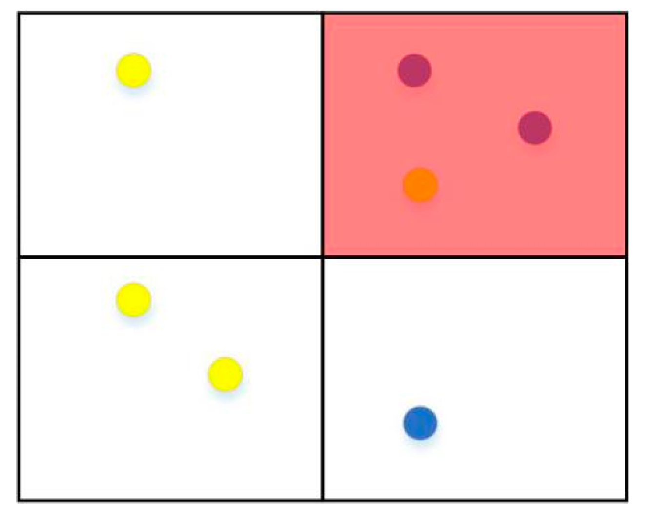
The blue points represent the buildings with type label “school” and the yellow points indicate the buildings with type label “residential buildings”. As a result, the red region is returned as the result of our top-1 query by matching the environmental information of each candidate Region-Of-Interest (ROI) for the query.
Ijgi 08 00287 g001
Figure 2. 
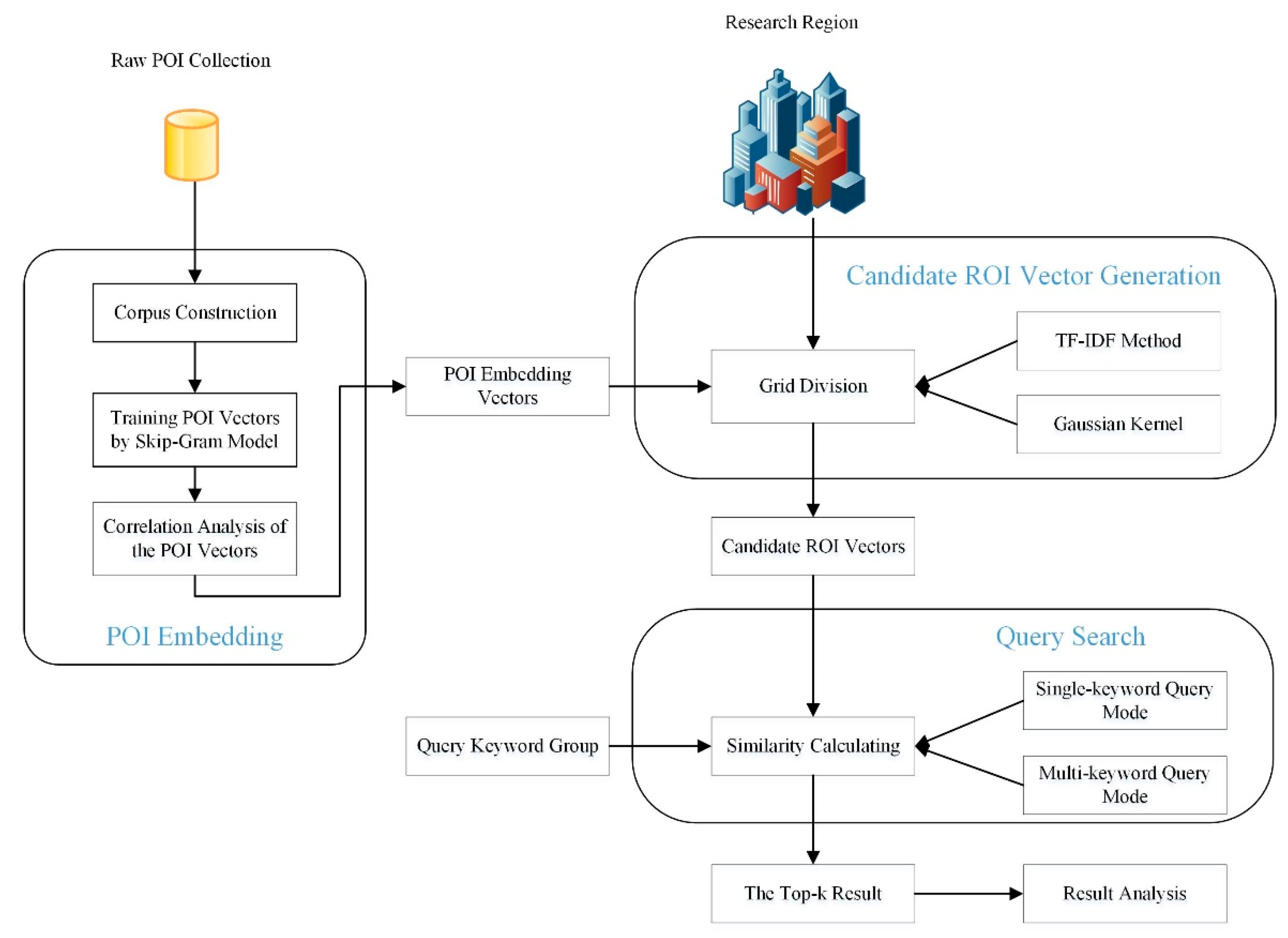
Workflow of the spatial keyword query of the ROI with the distributed representation of Point-Of-Interest (POI)s. TF-IDF, term frequency-inverse document frequency.
Ijgi 08 00287 g002
Figure 3. 
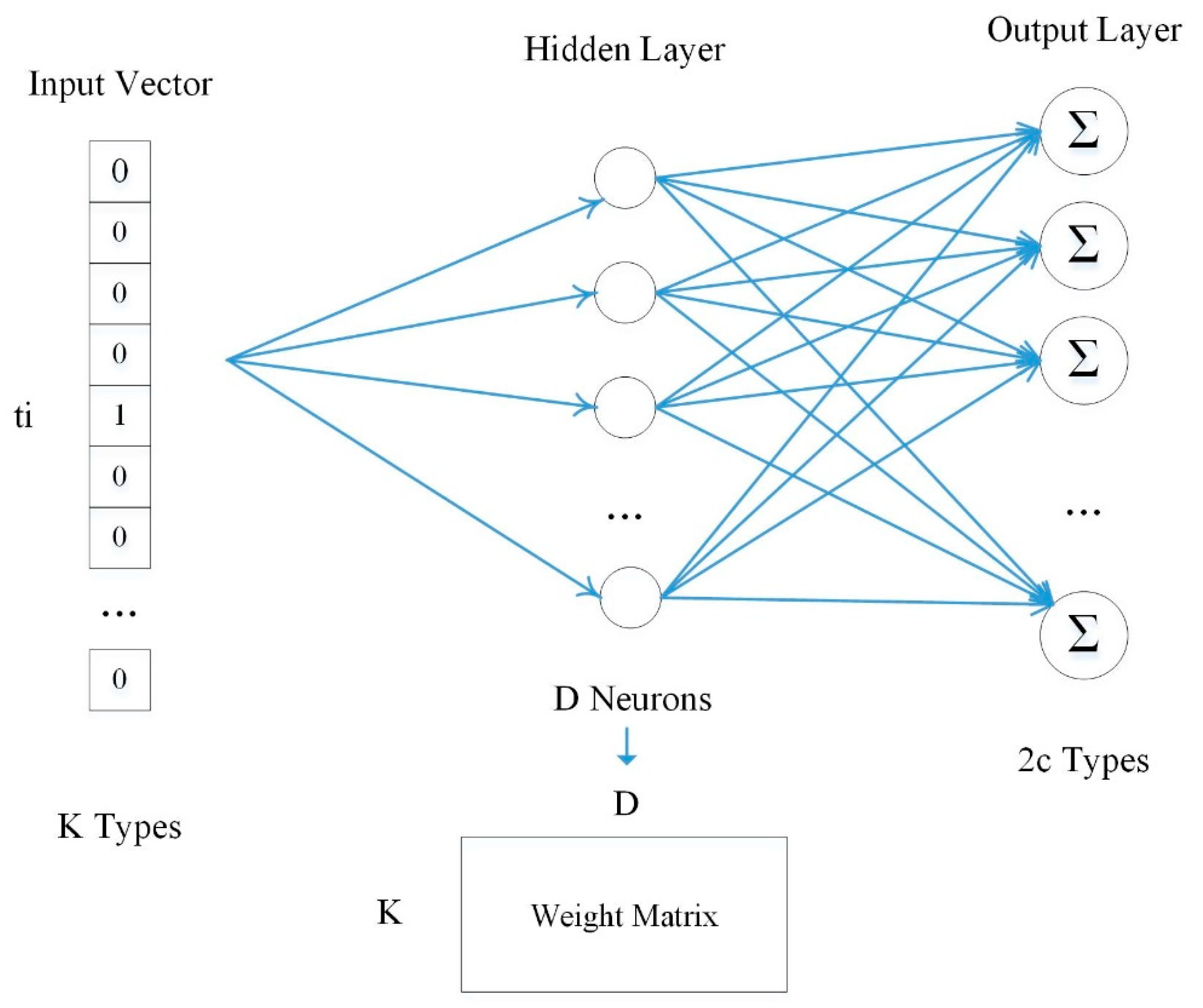
The Skip-Gram model. In the output layer, the input vector is the one-hot form where “1” represents the occupied position of the input type in the K types. In the hidden layer, D linear neurons are adopted and the D×K weight matrix of the neurons is the POI vector matrix. In the output layer, each output neuron uses a softmax classifier to predict the conditional probability of its context POI types, and the target is to minimize the loss.
Ijgi 08 00287 g003
Figure 4. 
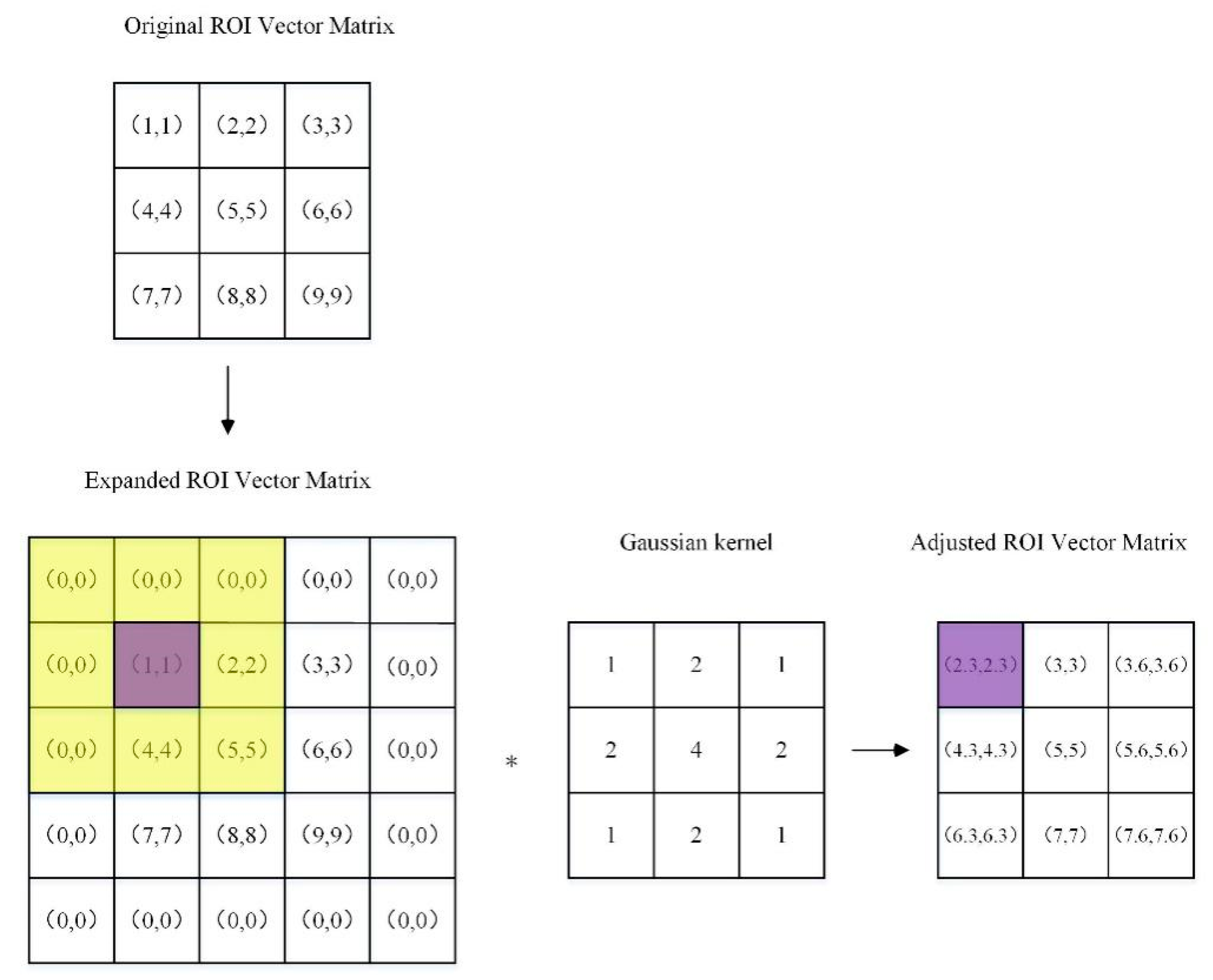
Gaussian kernel computing. The figure reveals that the first step of computing is to expand the original ROI vector matrix R(a,b) to the size of R(a+2, b+2), where the extended part is filled by the 0 vector. Meanwhile, with the convolution kernel weight corresponding to the 0 vector region set as zeros, the ROI vector in the edge of the original matrix can also be computed.
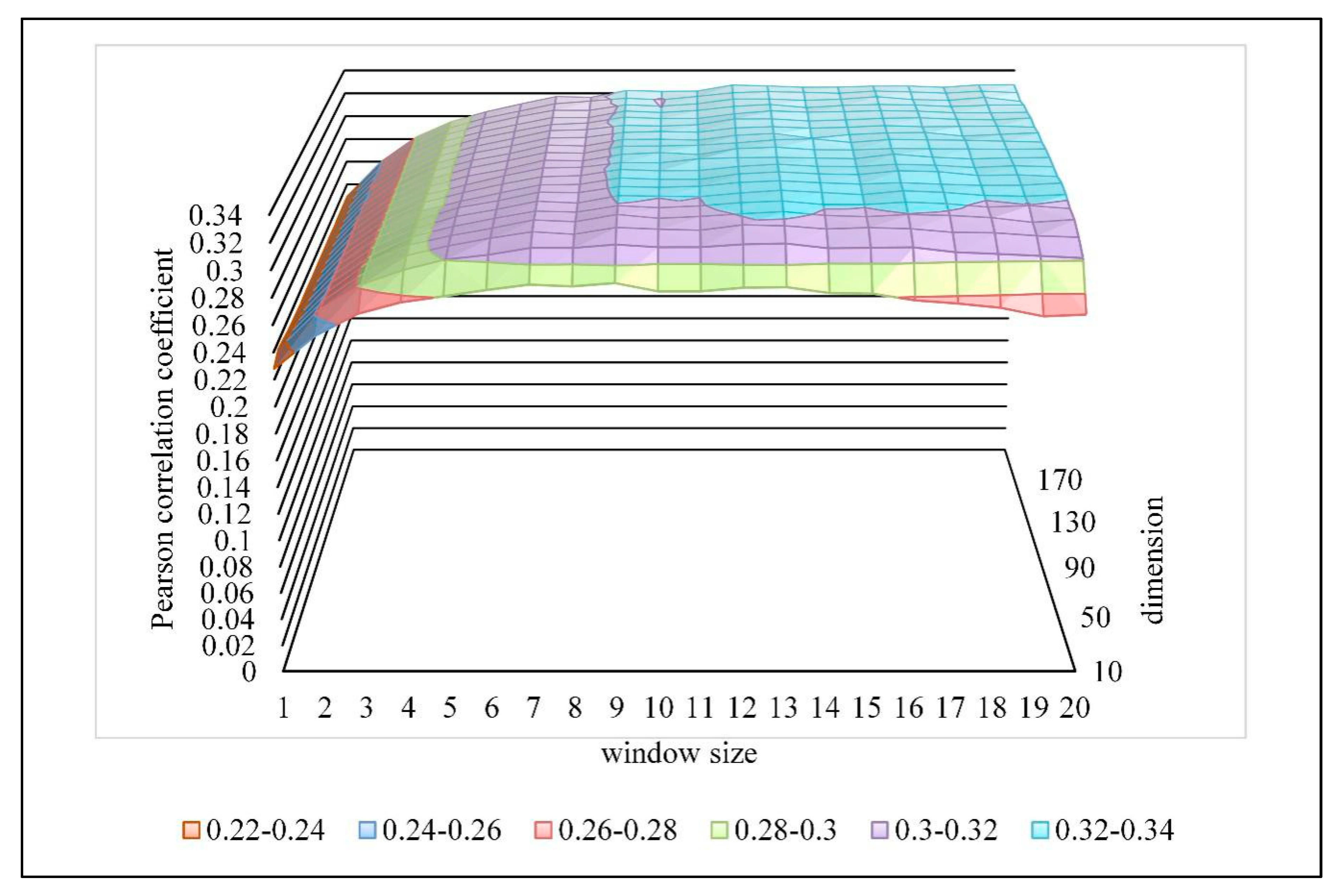
Ijgi 08 00287 g004
Figure 5. Parameter selection of the distributed representation of POIs. The X-axis is the window size, the Y-axis is the dimension, and the z-axis is the Pearson correlation coefficient corresponding to the first two. The different colors indicate the magnitude of the Pearson correlation coefficient.
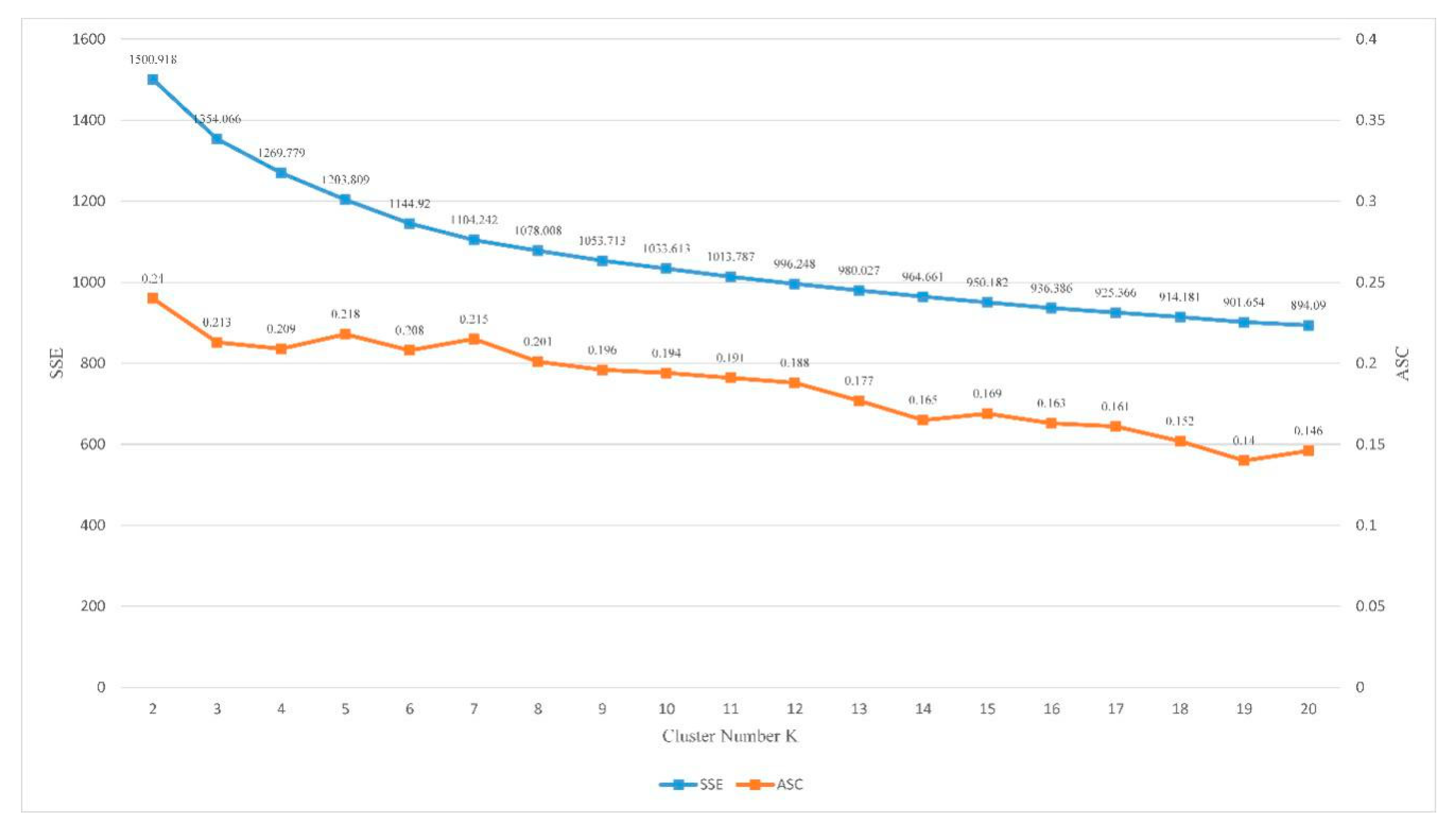
Ijgi 08 00287 g005
Figure 6. Change of average silhouette value (left y-axis) and error square sum (right y-axis) of clustering results (POI vectors) with increases of K value (x-axis).
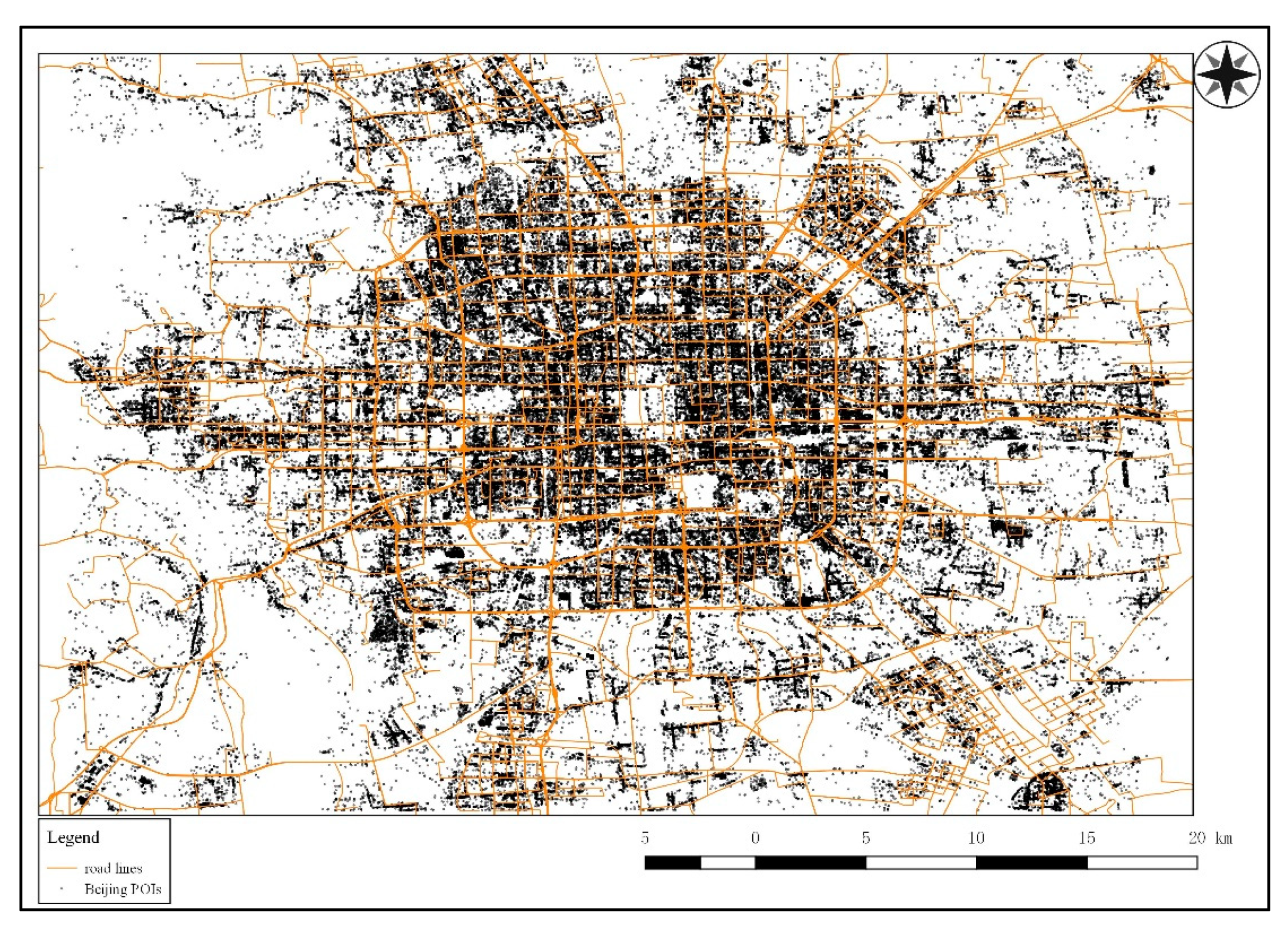
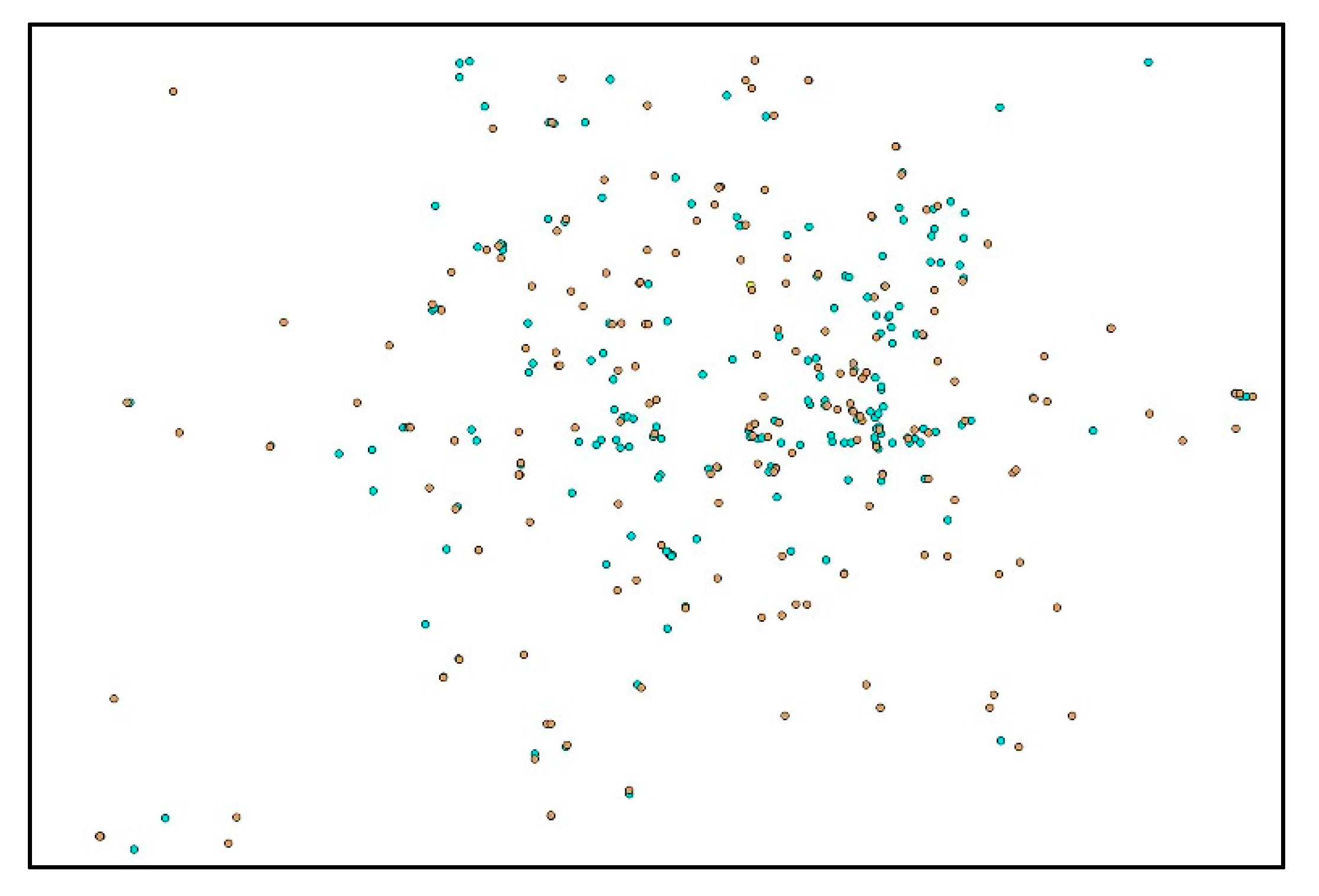
Ijgi 08 00287 g006
Figure 7. Research region. Yellow lines in the figure denote the main road data of Beijing and the small black dots indicate the POIs of Beijing.
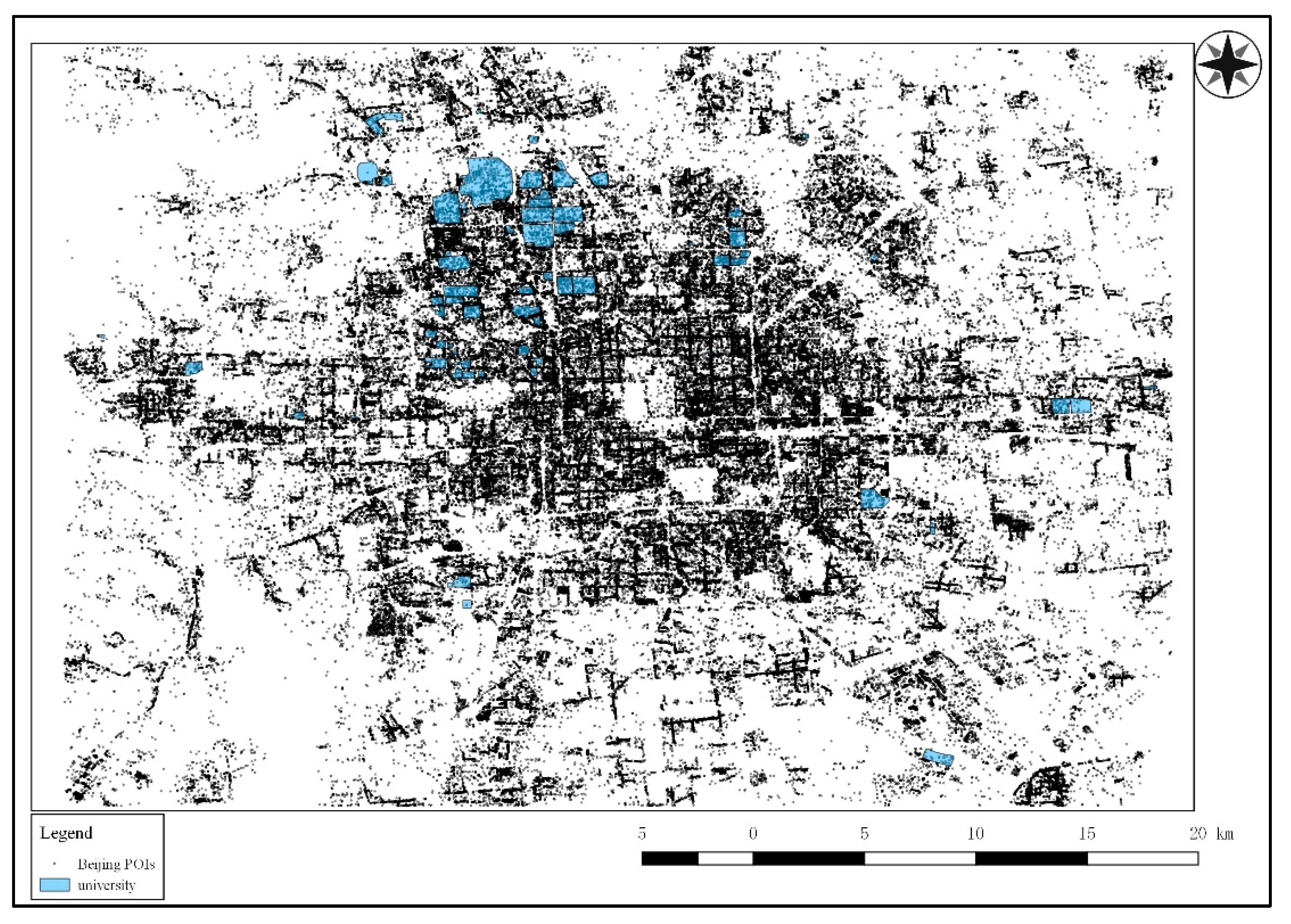
Ijgi 08 00287 g007
Figure 8. ROI validation set. The figure shows the distribution of the ROIs labeled “university”, represented by the blue regions in the research region. These were utilized to verify the effectiveness of the keyword query for the ROI of the corresponding label.
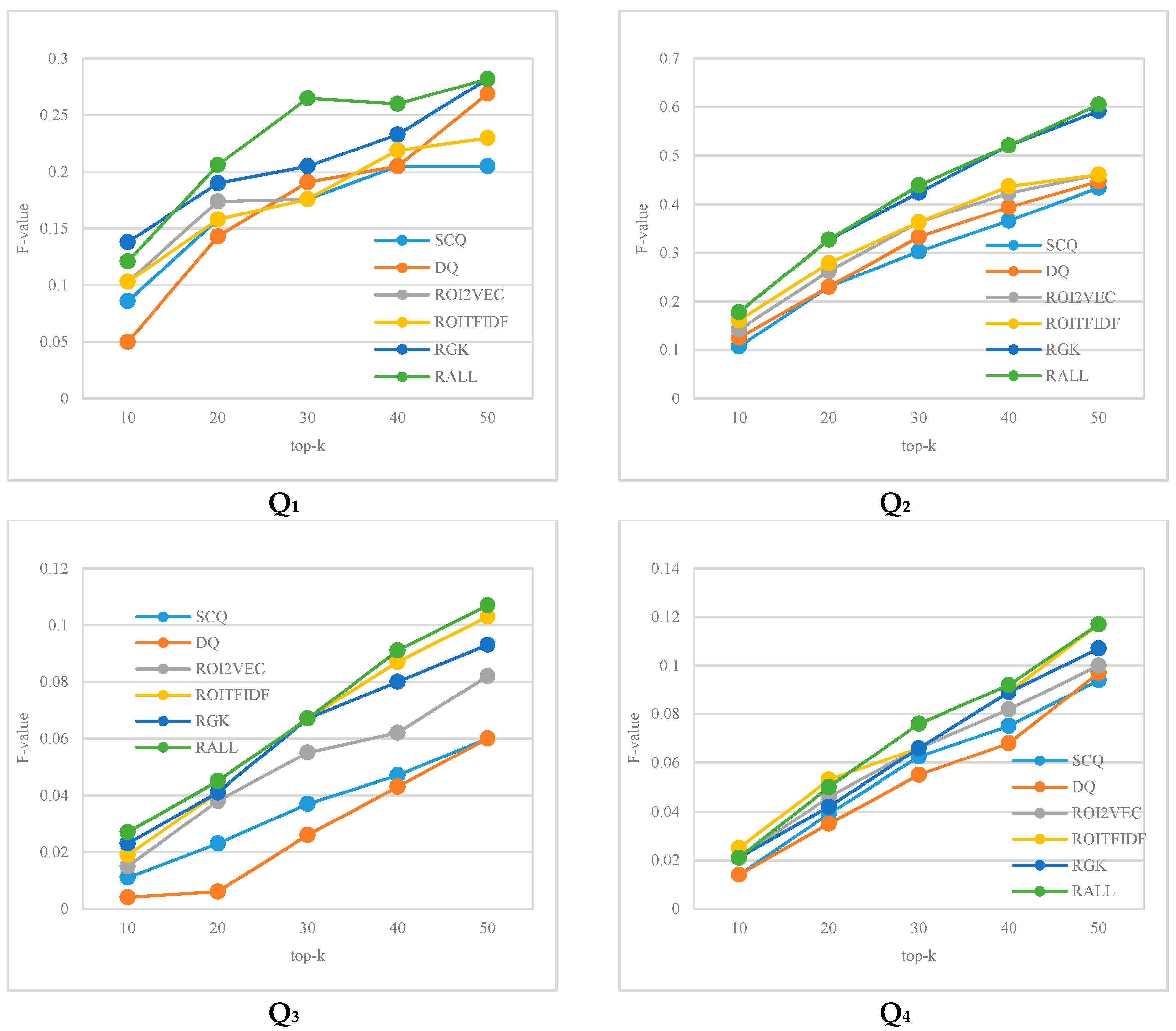
Ijgi 08 00287 g008
Figure 9. The performance comparison of the methods in Q1~Q4, which shows the change of the F-values (y-axis) of the query results with increases in the K value of the top-K query (x-axis).
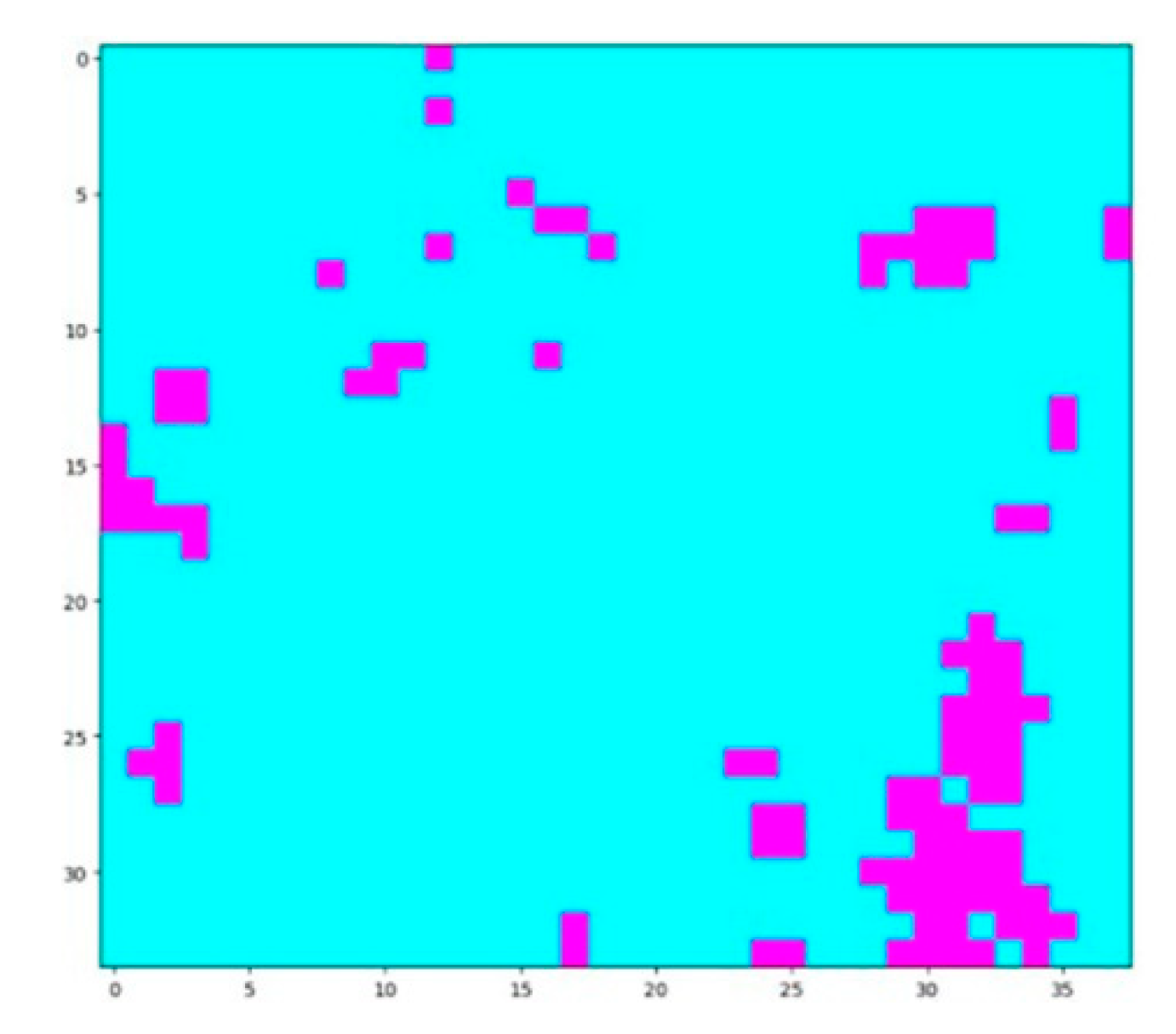
Ijgi 08 00287 g009
Figure 10. Original ROI rasterization. The labeled ROI occupied 106 grids in total in the research region (38 × 34 grids). The purple grids indicate the labelled regions.
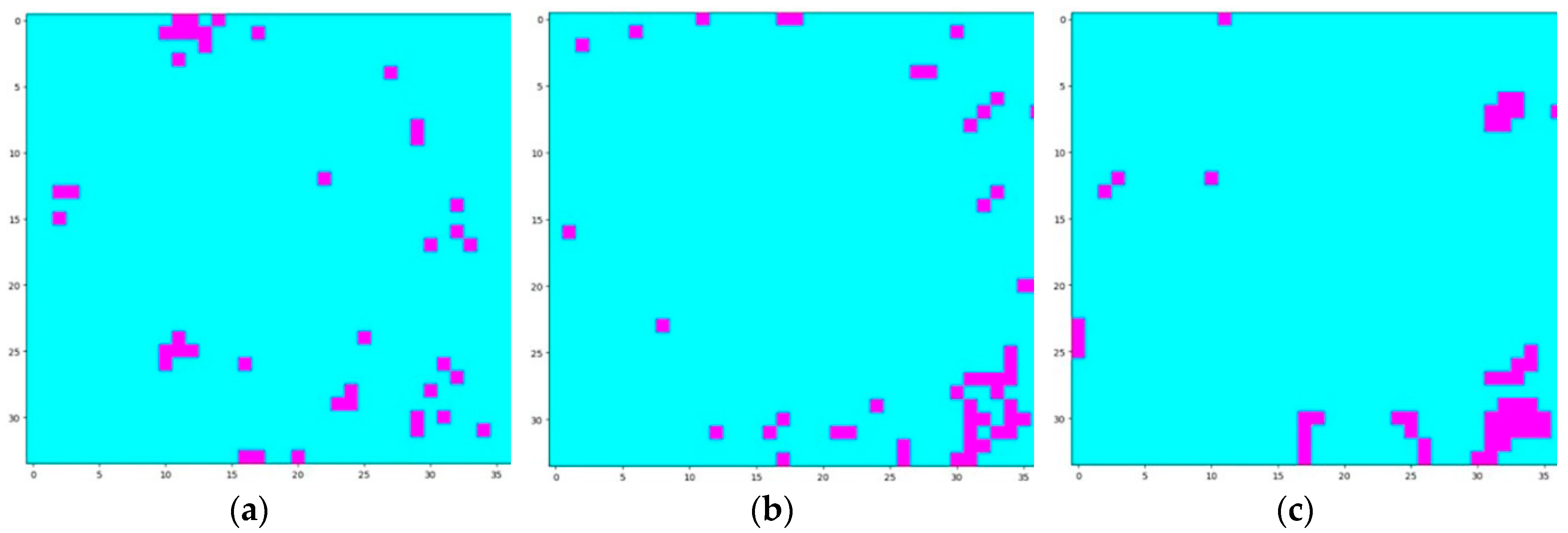
Ijgi 08 00287 g010
Figure 11. (a) Simple count query (SCQ) result of the top-50 ROI queries. (b) ROI vector (ROI2VEC) result of the top-50 ROI queries. (c) ROI2VEC + TF-IDF + Gaussian kernel (RALL) result of the top-50 ROI queries.
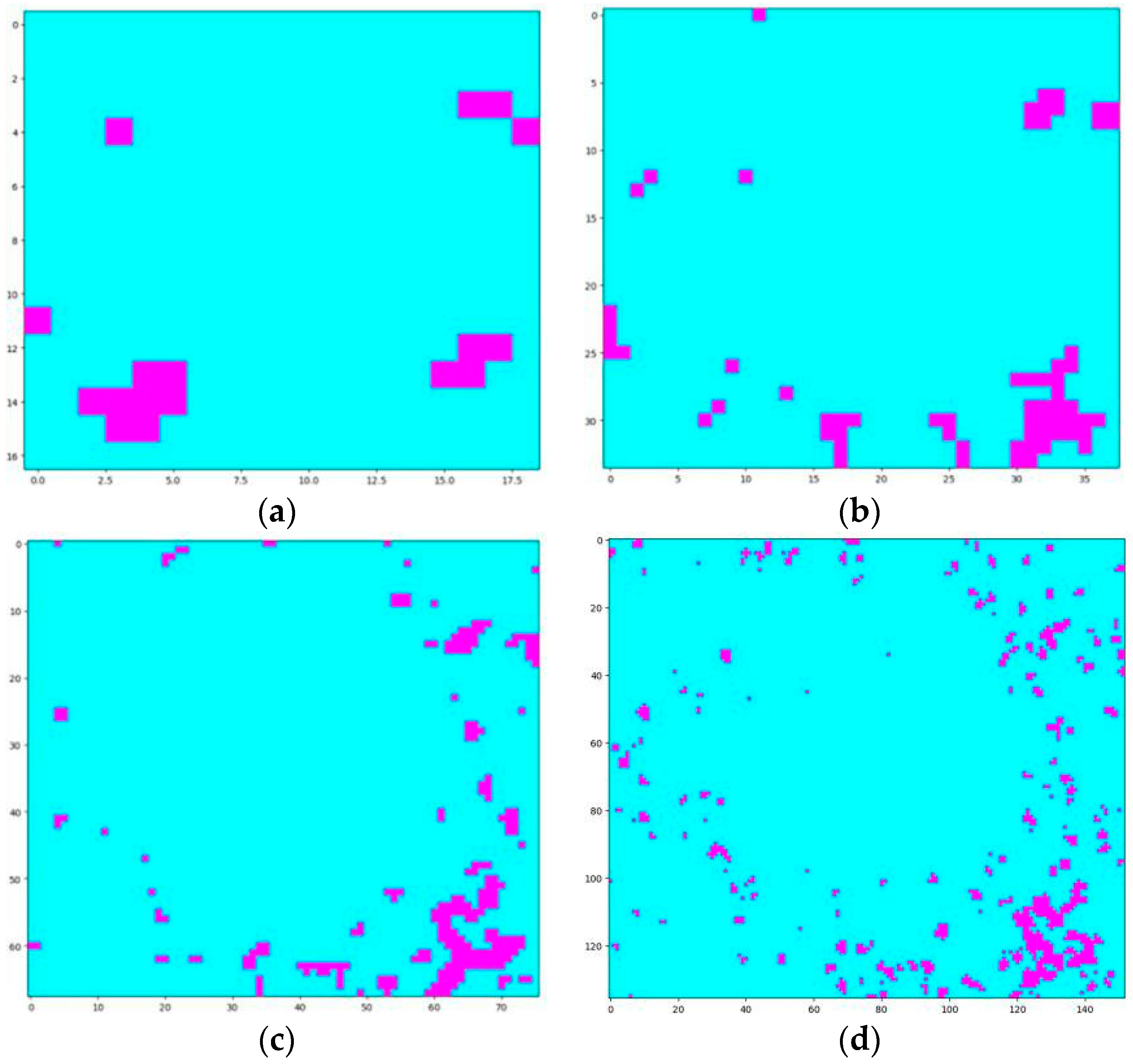
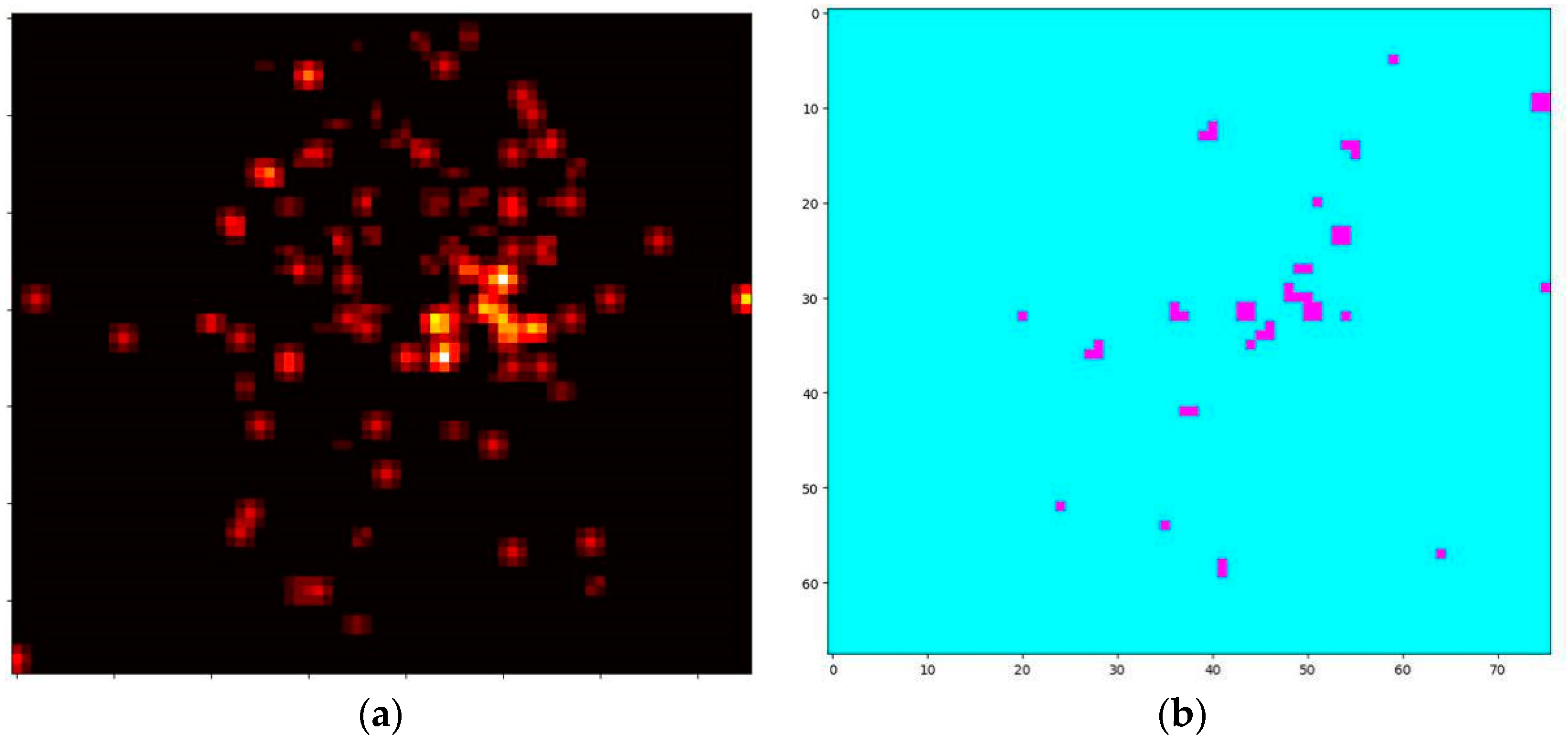
Ijgi 08 00287 g011
Figure 12. Q1 query results by RALL for the different sizes of the grids. (a) The 4 km2 size of the grid. (b) The 1 km2 size of the grid. (c) The 0.25 km2 size of the grid. (d) The 0.0625 km2 size of the grid. With the same query area ratio set for different tasks, the corresponding F-values were: (a) 0.141, (b) 0.339, (c) 0.297, and (d) 0.215.
Ijgi 08 00287 g012
Figure 13. In our research region, the blue POIs represent Starbucks while the yellow POIs represent the cinema. This figure shows their spatial distribution characteristics.
Ijgi 08 00287 g013
Figure 14. (a) The heat map of the POIs. It intends to reflect a combined relevance of the POIs of the type of Starbucks and cinema. Brighter grids denote a higher value of their combined relevance, i.e. both are densely distributed in this ROI, while the dark ones are the opposite. It is worth noting that the grids populated by only one type of POI do not show a very high correlation. (b) The top-50 query results by RALL. The top-50 query results are basically consistent with the brighter grids in (a), reflecting that our method can achieve good performance in the task of multi-keyword queries.
Ijgi 08 00287 g014
Table 1. Example of raw dataset P.
IDLocationType LabelOther Attributes
1(116.30, 40.41)library
2(116.43, 39.95)newsstand
3(116.46, 39.96)Starbucks
4(116.41, 39.98)clinic
Table 2. Symbols list.
SymbolMeaning
Pa collection of POI
pii-th POI
tii-th type label
Qa keyword query group
qii-th keyword in query
Ran ROI
Table 3. Type and count of top-level POI categories.
Top-level TypeIDCountTop-level TypeIDCount
Shopping Service176,038Financial Insurance Service1111,503
Life Service257,178Car Service1210,866
Transportation Facility337,404Accommodation Service137487
Catering Services436,001Public Facility145376
Government Agency530,484Car Maintenance Station152196
Science and Education Service626,726Road Auxiliary Facilities162189
Company721,011Famous Tourist Sites172090
Residence819,137Car Sales18649
Healthcare Service916,893Motorcycle Service19352
Sports and Leisure Service1016,210
Table 4. Clustering results. A higher percentage value means that the cluster has a higher proportion in top-level types, that is, it is more similar to this type. The numbers denote the type IDs of the top-level types, for example, “1” represents the “Shopping Service”.
KCluster12345678910111213141516171819
5C10.0%2.1%1.1%0.0%3.2%0.0%0.0%0.0%0.0%0.0%2.1%10.5%0.0%0.0%36.8%3.2%0.0%41.1%0.0%
C27.1%7.1%4.0%9.1%6.1%5.1%5.1%2.0%1.0%4.0%47.5%0.0%2.0%0.0%0.0%0.0%0.0%0.0%0.0%
C30.0%6.8%6.8%0.0%0.0%8.5%11.9%3.4%0.0%39.0%0.0%0.0%1.7%0.0%0.0%0.0%22.0%0.0%0.0%
C439.5%2.3%15.1%31.4%0.0%1.2%0.0%0.0%0.0%2.3%2.3%0.0%0.0%5.8%0.0%0.0%0.0%0.0%0.0%
C514.3%13.2%2.7%10.4%14.3%8.2%3.8%2.2%10.4%6.0%4.9%2.7%2.7%1.1%0.0%0.5%0.5%0.5%1.1%
7C10.0%0.0%0.0%0.0%2.3%0.0%0.0%0.0%0.0%0.0%2.3%11.4%0.0%0.0%39.8%0.0%0.0%44.3%0.0%
C25.0%5.0%5.0%7.5%3.7%1.3%6.2%2.5%1.3%3.7%56.2%0.0%2.5%0.0%0.0%0.0%0.0%0.0%0.0%
C30.0%9.3%9.3%0.0%1.9%3.7%14.8%1.9%0.0%29.6%0.0%1.9%1.9%0.0%0.0%5.6%20.4%0.0%0.0%
C449.3%1.4%0.0%39.1%0.0%0.0%0.0%0.0%0.0%5.8%0.0%0.0%0.0%4.3%0.0%0.0%0.0%0.0%0.0%
C522.3%18.2%1.7%17.4%0.8%2.5%4.1%0.8%7.4%6.6%9.1%2.5%3.3%0.8%0.0%0.0%0.8%0.0%1.7%
C69.1%9.1%59.1%4.5%0.0%4.5%0.0%0.0%0.0%0.0%4.5%0.0%0.0%9.1%0.0%0.0%0.0%0.0%0.0%
C70.0%5.7%3.4%0.0%32.2%21.8%1.1%4.6%11.5%10.3%1.1%1.1%1.1%1.1%0.0%1.1%2.3%1.1%0.0%

