Modeling Housing Rent in the Atlanta Metropolitan Area Using Textual Information and Deep Learning


1
Department of Geography, 2855 Main Drive, Fort Worth, TX 76109, USA
2
Statistics and Mathematics School, Yunnan University of Finance and Economics, Kunming 650221, China
3
Department of Computer Science, Eastern Michigan University, Ypsilanti, MI 48197, USA
4
Department of Landscape Architecture and Urban Planning, Texas A&M University, College Station, TX 77843, USA
*
Author to whom correspondence should be addressed.
ISPRS Int. J. Geo-Inf. 2019, 8(8), 349; https://0-doi-org.brum.beds.ac.uk/10.3390/ijgi8080349
Submission received: 28 May 2019
/
Revised: 22 July 2019
/
Accepted: 25 July 2019
/
Published: 2 August 2019
Abstract
:The rental housing market plays a critical role in the United States real estate market. In addition, rent changes are also indicators of urban transformation and social phenomena. However, traditional data sources for market rent prediction are often inaccurate or inadequate at covering large geographies. With the development of housing information exchange platforms such as Craigslist, user-generated rental listings now provide big data that cover wide geographies and are rich in textual information. Given the importance of rent prediction in urban studies, this study aims to develop and evaluate models of rental market dynamics using deep learning approaches on spatial and textual data from Craigslist rental listings. We tested a number of machine learning and deep learning models (e.g., convolutional neural network, recurrent neural network) for the prediction of rental prices based on data collected from Atlanta, GA, USA. With textual information alone, deep learning models achieved an average root mean square error (RMSE) of 288.4 and mean absolute error (MAE) of 196.8. When combining textual information with location and housing attributes, the integrated model achieved an average RMSE of 227.9 and MAE of 145.4. These approaches can be applied to assess the market value of rental properties, and the prediction results can be used as indicators of a variety of urban phenomena and provide practical references for home owners and renters.
1. Introduction
The rental housing market is a very important real estate market in the United States. Renter-occupied housing accounted for 35 percent of all US households in 2012, and a total of 43 million households by 2013 [1,2]. Based on information from Zillow, the total rent in the US has increased over recent years, reaching a record high of $485.6 billion in 2017 [3]. Investigation of trends in rental prices has great value for both practitioners and academicians. For rental property owners, it is critical to set appropriate prices in order to attract interest from potential renters, while for renters, it is most cost-effective to identify reasonable prices based on expected location and house condition.
For urban researchers, rent is a good indicator of urban structure and social phenomena. The classic bid rent theory in urban geography explains how land use and land price change as a function of distance away from the central business district (CBD) [4]. Based on this theory, a number of approaches have been developed to model urban land use process. The bid-rent land use model (BLUM) was proposed to consider spatial competition and utility curves of willingness to pay to solve the spatial competition problem [5]. Furthermore, observing rent changes over time facilitates greater understanding of the impacts of urban planning and land development projects on socio-spatial processes. For example, Immergluck (2009) examined how the planning and development of the Atlanta Beltline project corresponded with changes in price premiums and rents for locations in various geographical buffers around the Beltline [6]. In short, rents and housing prices were sensitive to the large redevelopment project, especially in lower-income neighborhoods; this resulted in high possibilities of gentrification. Lopez-Morales (2011) analyzed the gentrification process through ground rent based on the rent gap theory [7,8], and found that social capitalization of the ground rent was emphasized during the peri-central urban renewal process.
A number of methods have been used to model rent prices. Because rental values are determined by a variety of factors such as location, neighborhood characteristics, market conditions, and property-specific factors [9], assessing the rental values of residential properties is a complex and challenging process [10]. Among currently available methods, the hedonic pricing model is one of the most popular approaches. Many previous studies have used hedonic models to estimate the effects of environmental amenities or disamenities on rental prices [11]. For instance, Donovan and Butry (2011) investigated the effect of urban trees on the rental price of single-family homes in Portland, Oregon [12]. They found that an additional tree on a house’s lot increased the monthly rent by $5.62, while a tree in the public right of way increased rent by around $21. Baranzini et al. (2010) used hedonic models to estimate the influence of measured and perceived noise levels on property prices [13]. In addition, different interpolation approaches have been used to estimate property prices, such as inverse distance weighting, 2-D shape functions for triangles, kriging, and the fractal filtering method [14,15]. Meanwhile, spatial econometrics approaches such as spatial autoregressive (SAR) models have been used to account for spatial autocorrelation in house/rental prices. For example, Anselin and Le Gallo (2006) investigated the sensitivity of house prices to the spatial interpolation of air quality using spatial lag models [16]. Under conditions of spatial non-stationarity, geographically weighted regression (GWR) is a preferred method that considers local varying influences on dependent variables; it has been widely used in modeling house prices. Lu et al. (2011) used a GWR model to explore spatially-varying relationships between house prices and floor areas in London [17]. Huang et al. (2010) incorporated temporal effects into the GWR model to account for both spatial and temporal factors when modeling the real estate market [18]. Spatial models, such as kriging or Gaussian process regression (GPR), are important models that make predictions based on underlying spatial covariance; these generally work better than basic linear regression or other deterministic models.
Despite the popularity of regression models for analyzing house/rental price and its determinants, their usage is criticized because of limitations associated with fundamental model assumptions, feature selection, and the use of unstructured data [19,20]. In recent years, machine learning has introduced alternative econometric approaches for fitting and predicting house/rental prices [21]. Chen et al. (2016) summarized two main advantages of machine learning methods over traditional statistical methods [20]. First, statistical methods usually make strong assumptions concerning the randomness of measure errors of data (e.g., normal distribution), which may not always follow the real-world situation. Second, machine learning methods are able to capture high-order interactions among features and non-linear relationships between dependent and independent variables. Recent developments in deep learning additionally provide ways to better utilize unstructured data such as texts, images, and audio [22].
When predicting house rent, variables traditionally used include the square footage and number of bedrooms; additional features that make a difference to rental prices include interior design and decoration, floor plan, amenities, and unique upgrades. These features are usually documented in text form. It is challenging to capture such features using numeric variables. Deep learning learns through multiple layers of representations or features and produces state-of-the-art results based on both structured and unstructured data [23,24,25]. Accordingly, deep learning techniques have been successfully used for mining textual information in many fields; nonetheless, their application in rental market modeling and prediction is still limited. With the recent rapid development of house/rental information exchange platforms such as Craigslist, user-generated rental listings provide big data that cover wide geographies and are rich in textual information. Integrating both spatial variables and textual information in rent modeling may advance understanding of the dynamics of rental markets. In addition, such a model can facilitate greater understanding of different housing submarkets. Hence, in this study, we aim to develop and evaluate models of rental market dynamics using deep learning approaches that incorporate spatial and textual data.
2. Method
2.1. Study Area
Atlanta is the capital of, and also the biggest city in Georgia, US. Its metropolitan area is the ninth largest in the nation, with a resident population of around 5.9 million in 2017 [26]. The average rent in metropolitan Atlanta increased by 4.4 percent in 2017, ranked as the fifth fastest increase nationwide [27]. In the past few years, a number of large-scale developments occurred in the city, which significantly impacted residential property value and rental prices [6].
2.2. Data
The data used in this study was collected from Craigslist, a classified advertisement website for information posting and sharing. In recent years, Craigslist data have become important sources for urban studies. As pointed out in Boeing and Waddell (2017), a researcher can scrape publicly available data such as Craigslist listings for non-commercial uses that neither repackage nor relist the data [1]. Accordingly, they used nationwide Craigslist rental housing lists to analyze rental housing markets across the US. Hu et al. (2018) used Craigslist housing advertisements to extract local place names [28]. In this study, we crawled posts related to the apartment/houses for rent in Atlanta from April to December 2018. Information such as the date of posting, latitude and longitude, bedroom number and square footage, short and long descriptions of the property, and links to figures were collected. The raw data was stored as comma-separated text and only used for research purposes.
2.3. Data Cleaning
The raw dataset contained a lot of information noise. For one, duplicated posts are very common on Craigslist, as people tend to repost advertisements to move them to the top of the list and therefore receive more attention. Accordingly, we first removed duplicated posts. In addition, we filtered posts with no geographic location. Another characteristic of Craigslist posts is that a number of posts include unreasonably low or high prices (e.g., spam, deliberate mislabeling to attract attention, or mis-posted information). To remove these records, we calculated a threshold for defining outliers based on local average rental prices, then removed identified outliers from the dataset. For posts missing either square footage or bedroom number, the missing value was imputed based on the correlation between these two variables. Posts lacking both square footage and bedroom number were discarded. In the cleaned dataset, each data entry was expressed as a tuple (ft2, bd, lon, lat, sd, ld, p), where lon and lat were the longitude and latitude coordinates of the property, ft2 and bd were square footage and bedroom number respectively, sd and ld represented short descriptions and long descriptions, and p was the rental price. Short descriptions usually consisted of the post title, while long descriptions contained the main text the property owner used to describe the property.
2.4. Experiment Design
For the evaluation of model performance, we designed a three-experiment framework that assessed model fit.
2.4.1. Exp. I: Single Model without Textual Information
In this experiment, we first modeled rental prices using common interpolation methods, including inverse distance weighting and kriging (Gaussian process regression). Spatial interpolation algorithms follow Tobler’s First Law of Geography [29]; thus, the value at a point of interest is estimated as the weighted sum of values at surrounding data points such that closer neighbors contribute larger weights. Inverse distance weighting (IDW) explicitly relies on the First Law of Geography by setting the weight as the inverse of the distance (Equation (1)).
where represents the unmeasured value to be calculated at the data point of interest , is the spatial Euclidean distance between and , is an exponent that influences the weighting of , and is the number of nearest neighbors that contribute to the point of interest. In this experiment, we tested three -values, i.e., the first, second, and third orders, in order to evaluate the influence of the exponent on modeling outcomes. When making predictions, we considered the 12 nearest neighbors.
Kriging or Gaussian process regression is modeled by a Gaussian process governed by prior covariance functions. Kriging is named after the South African mining engineer D. G. Krige [30], who first presented this method to improve the precision of predictions of gold concentration in ore bodies, and is known to be the optimal or best linear unbiased prediction. The main idea of kriging is to analyze the correlations among the residuals of data points. In this method, can be decomposed into a deterministic trend function and a real-valued residual random function . That is,
Similar to IDW, kriging also estimates the residual at as the weighted sum of residuals at surrounding data points, that is . The weight is derived from a covariance function or variogram, which is utilized to characterize the residual component. There are three classical versions of kriging, each employing different assumptions: Simple kriging, ordinary kriging, and universal kriging. Simple kriging assumes the stationarity of the first moment over the entire domain with a known mean ; ordinary kriging assumes a constant unknown mean only over the search neighborhood; and universal kriging assumes a general polynomial trend model, such as the linear trend model
In this study, we tested the ability of both ordinary and universal kriging to estimate rental prices. When using universal kriging, we adopted a linear trend model with f(x) = x. In addition, we used Gaussian process regression to simultaneously model four variables: Latitude, longitude, bedroom number, and square footage. The covariance functions or kernels considered in our experiments are all Gaussian, i.e., squared exponential covariance functions. Because kriging and GPR are computationally intensive, we sampled 1600 feature points for training the models. These models were trained and validated on the same data splits to make sure their outcomes were comparable.
Next, we selected popular linear, nonlinear (not ensemble), and ensemble algorithms to model rental price based on location, square footage, and bedroom number. Each algorithm has its own advantages. For problems that are inherently linear, linear models are fast and simple. Nonlinear algorithms can handle problems that are linearly inseparable. The performance of nonlinear algorithms may vary depending on the nonlinear characteristics of the feature space. Ensemble models combine several base algorithms to achieve an optimal predictive model. We tested a few different algorithms from each category. The linear algorithms tested in this study consisted of linear, lasso, ridge, elastic net, and stochastic gradient descent regressions. Lasso, ridge, and elastic net models provide approaches for regularizing models so as not to overfit the training dataset. Ridge regression penalizes the sum of squared coefficients while lasso regression penalizes the sum of absolute values. Elastic net is a convex combination of ridge and lasso.
The nonlinear algorithms (not ensembles) applied in this study included K-nearest neighbor algorithm (k-NN), regression tree (RT), multilayer perceptron (MLP), and support vector regression (SVR). k-NN is a very useful non-parametric model that does not assume any underlying data distribution; its prediction is based on the most similar k-neighbors in the training set. RT splits samples into relatively homogeneous sets based on the most significant splitter for input variables, with the terminal nodes containing the predicted output values. MLP is an artificial neural network composed of an input layer that receives feature signals, an output layer that makes a prediction, and several hidden layers. MLP is a powerful supervised learning model. SVR is based on a support vector machine, using the concept of maximal margin to make predictions.
Finally, the ensemble models tested in this project include AdaBoost, bagged decision trees, random forest, extra trees, and gradient boosting machines. Ensemble models combine decisions from multiple models to improve final performance. These models usually include two general approaches, bagging and boosting. Random forest and bagged decision trees are considered bagging approaches. Bagging usually samples the training data set with replacement, then creates a model for each sample. The results of those multiple models are combined and the average is used for final predictions. AdaBoost and gradient boosting machines are considered to use the boosting approach. Boosting is a sequential approach in which a first model is trained on the entire dataset, and the subsequent models are built by fitting the residuals of previous models. Such iterations allocate higher weights to observations that were poorly predicted by the previous model [31].
In this project, the top-performing algorithms were recorded and reported. To fine-tune performance, we also conducted a grid search for the top ten models. We conducted two groups of tests: One using the same training and validation split as with the IDW and kriging models, the other using the full dataset, which is consistent with the experiments described below.
2.4.2. Exp. II: Single Model Based on Textual Information
Textual information embedded in the short and long descriptions is critical when modeling rents. For instance, factors such as decorations, neighborhood, amenities and unique upgrades, and interior design cannot be reflected in square footage and bedroom number, yet contribute significantly to rental price. To capture information about room quality for the purpose of predicting price, we used three types of models: Latent semantic analysis (LSA), recurrent neural network (RNN), and convolutional neural network (CNN).
LSA is a technique for creating a vector representation of textual information. We first convert the property descriptions D to a matrix of word counts T, with rows being individual properties and columns being all possible words in the descriptions. Then, the matrix T is transformed based on tf-idf equations as below:
Term frequency (tf) counts the number of times a word t occurs in a property description d. The inverse document frequency (idf) is an indicator of how much information the word t provides, measured as the frequency of word t across all documents D.
Next, we apply singular value decomposition (SVD) to the transformed matrix T to lower its dimensionality. Specifically, we decomposed the matrix T into three matrices where U and V are orthogonal and is a diagonal matrix containing k singular values. In this study, we used k<<k to approximate T . The new matrix was used to predict prices.
RNN. Traditional neural networks treat input words independently. However, when modeling textual information, spatial adjacency such as ‘close to downtown’ or ‘five minutes away from airport’ is meaningful; this adjacency cannot be captured by traditional neural networks. RNN, however, can make use of the sequential information. It trains a model for every input word sequentially, with the output from the current input word depending on previous computational results. Such a process can be expressed as:
where is the hidden state at time t. It is a function of the current word input , multiplied by a weight matrix W, and the hidden state derived from previous words at time , multiplied by its hidden state weight matrix M. By maintaining the internal hidden state ht and sharing this parameter across all time steps, an RNN is able to remember past information and repeatedly occurring patterns.
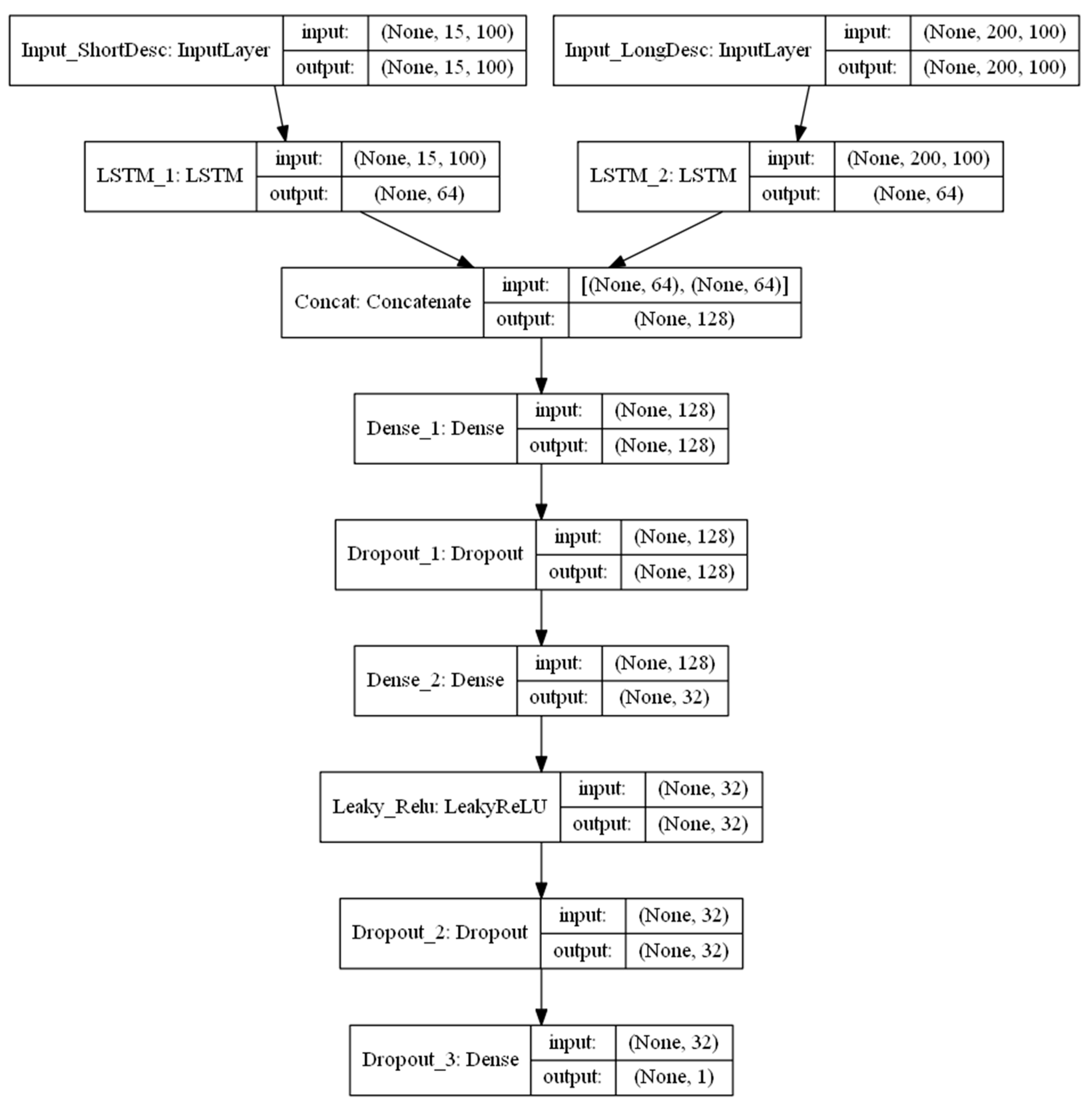
In this study, we first converted each word from the property descriptions into vector spaces using Global Vectors for Word Representation (GloVe) [32]. This step maps words with similar meanings (e.g., house and apartment) to similar vector representation. Next, because RNN requires each input batch to have the same length, we padded each description with zeros so that the resultant vectors had the same length. We respectively used 15 and 200 vector lengths to pad short descriptions and long descriptions. Then, vector spaces for short and long descriptions were connected to two long-short term memory networks (LSTM). LSTM is a particular architecture of RNN designed to minimize the vanishing gradients problem, which is caused by the fading memory of past learned patterns over time [33]. Outputs from the two LSTM models were concatenated and sent to a densely connected network for final predictions. The detailed scheme of the model is provided in Figure 1.
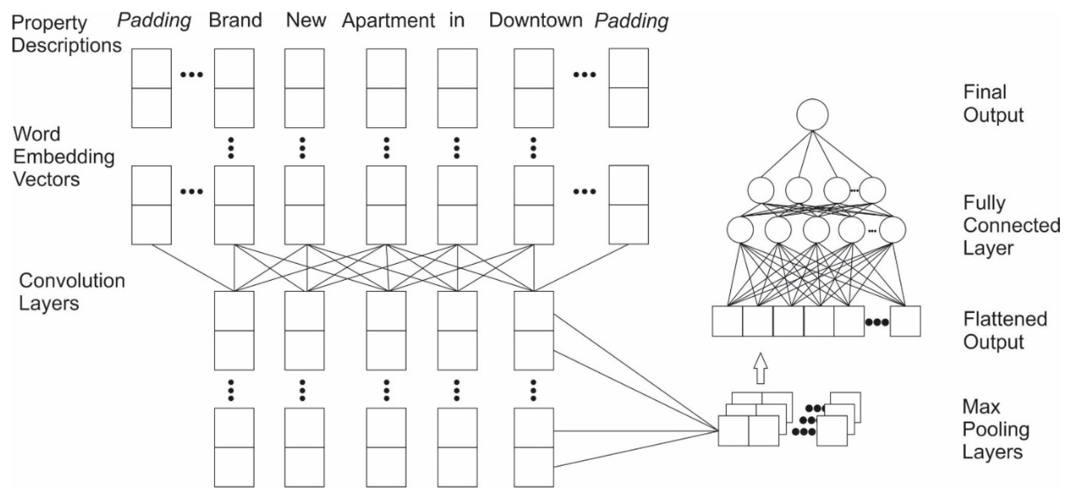
CNN. The convolutional neural network (CNN) is inspired by biological processes in the visual cortex of animals, and thus commonly applied to image recognition. Since a one-dimensional-CNN scans data in a one-dimensional and sequential manner, it can also be used to capture sequential textual information. We tested a 1D-CNN for capturing relationships between adjacent words. A typical CNN network usually contains a convolutional layer, a pooling layer, and a fully-connected layer. We created our network following this paradigm. First, as with LSTM-RNN, we converted the words in property descriptions into vector spaces using GloVe. Similarly, word sequences were padded to form a homogeneous vector space. We then employed a 1D convolution layer to slide the filter over each vector space. As the core building block of a CNN, the convolution layer partitions input into partially overlapping regions and utilizes convolution operations to explore these regions, which emulates the response of an individual cortical neuron to visual stimulus. We also applied the activation function ReLU (defined as ) to introduce non-linearity into the network (Figure 2).
Next, we applied a max pooling layer, which takes the maximum value in each one-dimensional window as the output. This process decreases the number of features while retaining the most important information. Finally, we flattened the combined outputs from pooling layers and concatenated layers from both short descriptions and long descriptions to construct a fully-connected network (Figure 3).
For both RNN and CNN, we used Adadelta as the optimizer and mean absolute error (MAE) as the loss function. Adadelta is a robust optimizer, which adapts the learning rates used in stochastic gradient descent [34]. Model performance was evaluated by cross-validation. In addition, for both RNN and CNN, we used Leaky ReLU (Equation (6)) at the second-to-last layer rather than the common ReLU activation function. Leaky ReLU allows a small, non-zero gradient when the neurons are not active. This change helped to maintain a small fraction rather than zero when the input was negative, which was helpful in Exp. III when we fed outputs from the second-to-last layers into other machine learning models (e.g., random forest).
2.4.3. Exp. III: Combined Models Using both Numeric and Textual Information
We combined numeric information (e.g., location, bedrooms, and square footage) and textual information (short and long property descriptions) derived from Exp. II to jointly model rental prices. We first kept the weights trained in Exp. II, transferring them directly to Exp. III. Notably, the second-to-last outputs of LSTM and 1D-CNN are 32-dimensional vectors that embed the information derived from apartment descriptions. In order to reduce the dimensionality of these vectors, we extracted the major components using principal component analysis (PCA). All features were trained on a number of models in order to evaluate model performance.
We used multiple indicators to assess the models; specifically, the mean absolute error (MAE), root-mean-square error (RMSE), and mean absolute percentage error (MAPE). Both MAE and RMSE evaluate absolute error, while MAPE measures relative error [35].
where Oi denotes the observed property price, Pi denotes the estimated property price, and N denotes the number of samples.
3. Results
A total of 351,230 raw records were collected from Craigslist for the Atlanta Metropolitan Area. After preprocessing as described in the methods section, we obtained 76,487 observations in total. Table 1 shows descriptive statistics for rental properties listed in the top ten counties as ranked by average listing price. Fulton, Dekalb, and Gwinnett are the most expensive areas, with average rental prices of $1509, $1301, and $1238, respectively. In all counties, properties with two bedrooms are the most common rental housing type on the market. Most of the rental properties are located in Fulton and Dekalb counties. Figure 4 shows the spatial distribution of rental price. In general, areas in central and northern Atlanta, such as Midtown, Buckhead, and Downtown, show higher rental prices than the rest of the metropolitan area.
Table 2 shows interpolation results from the IDW and kriging methods. We compared model performances for six models, i.e., three IDW methods, two kriging models based on only locational information, and one kriging (or Gaussian process regression) model incorporating location, bedroom number, and square footage. The Gaussian process regression (GPR) achieved the best accuracy, while ordinary kriging and universal kriging worked better than IDWs. Of the three IDW models, the first order IDW performed better than the second and third orders.
In addition, we evaluated model performance based on two groups of training-validation splits. The first group was a 10%–90% split for training and validation out of 16,000 randomly sampled data points, while the second group was an 80%–20% split for training and validation out of the full dataset. The reason we used two groups is because kriging, especially four-variable GPR, is a very computationally intensive method; sampling a small fraction of feature points for training reduces that burden. To ensure the kriging and machine learning models were comparable, we use the same training-validation splits for the common machine learning models. For the proposed deep neural network for review texts, we used a more traditional split proportion (i.e., 80% of observations in the training set) to include more data for training. Exp. II and Exp. III are all based on this 80%–20% split.
When comparing interpolation methods with machine learning approaches, the ensemble methods such as random forest, bagging, and gradient boost regression showed better performances. Nearest neighbor approaches were also slightly better than the interpolation methods. Comparing the small and large training sets revealed that, as we expected, the larger training set produces better accuracy (Table 3).
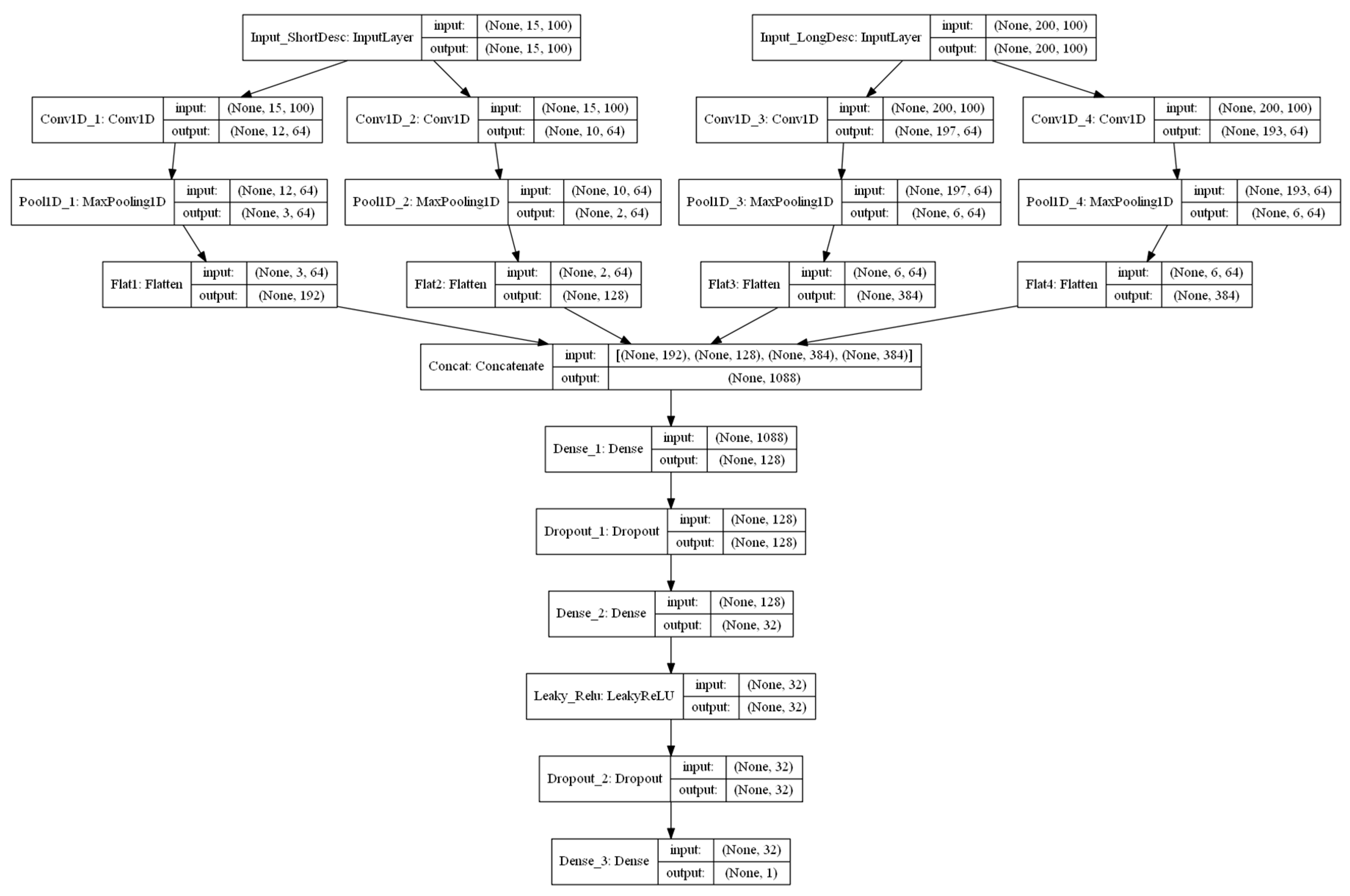
Similarly, we evaluated performances of the models from Exp. II. Figure 5 and Figure 6 show model structures and tensor dimensions for each layer in the CNN and RNN models respectively. In the CNN model, when conducting the 1D-convolution, we chose different lengths for the 1D convolution windows (i.e., kernel sizes) for short descriptions (four and six kernels) and long descriptions (four and eight kernels), respectively. In Figure 5, the layers Conv_1D, Conv_2D, Conv_3D, and Conv_4D have four, six, four, and eight kernels, respectively. After convolution and max-pooling, four layers were concatenated and connected with two densely-connected layers before the final output. In the RNN model, the short descriptions and long descriptions were connected with LSTM layers. Outputs from the LSTMs were concatenated and connected with two densely-connected layers before generating the final output. For both LSTM and 1D-CNN models, the final output was the predicted rental price, while the second-to-last layer was a 32-dimensional vector consisting of numerical information derived from textual descriptions.
Table 4 shows the results of Exp. II. Although the performance of models based on textual information was weaker than that of models based on numeric predictors, relatively good fits were achieved with textual information alone (without latitude and longitude, bedroom, and square footage). For latent semantic analysis (LSA), the MAE was 211.7 and the RMSE was 311.7. The RNN-LSTM and 1D-CNN models showed better performance than LSA, with MAE values of 196.8 and 208.9, respectively.
We tested whether the model prediction results were sensitive to the presence of keywords describing important characteristics of the property. Namely, we extracted certain keywords from the datasets and simulated records having the same long descriptions but different short descriptions (Table 5). We used the RNN model to predict prices. The model successfully captured textual information about bedroom numbers and important local destinations. The model also reflected that descriptive phrases such as “luxury apartment” tended to predict higher rent than phrases such as “good condition”.
In Exp. III, we considered textual information together with numeric variables. Specifically, we extracted model outputs from the second-to-last densely-connected layer as latent representations of property descriptions and concatenated these latent variables with the numeric variables. We then tested the ability of several models to predict rental prices from the concatenated variables (Table 6). Overall, the joint models with integration of textual and numeric information demonstrated better performance. The MAE of the best model was reduced to 145.4, and the average RMSE dropped to 227.967. Similarly, once we introduced textual information and extracted the top principal components, the performance of linear models increased significantly. This suggests that textual information played an important role in joint models.
4. Discussion and conclusion
The rental housing market is a very important part of the real estate market, and has received considerable attention from scholars. Many previous studies focused on identifying the driving factors of rental prices rather than modeling, predicting, and mapping the spatial distribution of prices [36]. Practically, models that accurately predict rental price can help property owners’ better price their rental properties and assist tenants in finding places to live with reasonable prices. In this study, we modeled rental prices in Atlanta based on Craigslist data. Craigslist is an important rental listings platform that has become increasingly popular for exchanging information related to rental housing; it provides rich rental information covering wide geographies, which makes the fine-scaled spatial-temporal assessment of rental value possible.
In summary, in this study, we tested a number of common machine learning approaches and developed deep learning models to predict rental prices. We utilized locations, house attributes, and textual descriptions in these predictions. Our experiments demonstrated that machine learning approaches can achieve good accuracy in estimating rental price solely based on Craigslist data. In particular, ensemble models achieve better accuracy than common interpolation methods. Deep learning approaches have advantages in handling textural information along with numeric information. Using only advertisement titles and descriptions, our models achieved an average MAE of 196.760. Another important lesson learned in the course of this study is to fuse different types of features through feature concatenation. Namely, by fusing textual data with numeric information, we effectively reduced the overall errors of our models.
In this study, some ensemble methods (random forest, bagged decision trees) performed better than the kriging, while other approaches (KNN, CART) were not as good. Kriging estimates the residual at a point of interest as the weighted sum of residuals at surrounding data points, and is based on the variogram technique. The main idea of the variogram relies on the assumption that the spatial relation of two sample points does not depend on their absolute geographic location, but only on their relative locations. However, real-world data may not follow this assumption. Such results are consistent with previous research comparing common machine learning approaches for interpolation tasks. Appelhans et al. (2015) found that machine learning approaches such as stochastic gradient boosting, random forest, and neural networks perform better than kriging in quantitative evaluations [37].
For the processing of textual information, we compared three methods, i.e., latent semantic analysis (LSA), recurrent neural network based on LSTM, and 1D-convolutional neural network (1D-CNN). The matrix decomposition method LSA achieved moderate accuracy, whereas the deep learning models LSTM and 1D-CNN achieved better results. The superior performance of deep learning models can be ascribed to their ability to capture sequential information. LSTM and 1D-CNN showed similar performance, with LSTM being slightly better. In addition, both LSTM and 1D-CNN tended to overfit the training model. Dropouts significantly improved the performance of both models.
There are a few limitations inherent in this study. First, the model was trained and tested based on data from the city of Atlanta. Patterns learned from this data may not be applicable to other contexts. Future studies can explore additional geographic areas and apply the model transferable learning capabilities to other cities. Second, most Craigslist rental posts also include images of the property, which were not used in our models. Images may provide valuable information concerning room/house condition and that otherwise predicts the rental price. In our future work, we will test whether adding such graphical information can improve the model fit.
In this study, we used data from Craigslist rental listings in Atlanta to predict rental prices. When constructing the models, we combined information including location, house attributes, and textual descriptions. Our experiments demonstrate that machine learning approaches can achieve high accuracy in estimating rental prices solely based on Craigslist data. In particular, textual information contributes to lower overall errors. LSTM and 1D-CNN performed better than LSA at modeling textual information. As a result, we used the model outcomes from LSTM together with numerical attributes to construct the final model. The final model achieved a mean absolute error of 145.358. Although the established model can effectively predict rental prices, its performance can be further improved by including data from multiple cities, such that the constructed model would be applicable to other geographic areas. In our future work, we will also consider using photo inputs and test if such information helps to further improve model performance. The results of this study can be used to model rental prices, assist research in housing dynamics, and provide practical references for home owners and renters to list and find properties at a reasonable price.
Author Contributions
Xiaolu Zhou conceived the ideas and collected the data. Xiaolu Zhou and Weitian Tong analyzed the data and interpreted the results. Xiaolu Zhou and Dongying Li prepared the manuscript and conducted critical revisions with input from Weitian Tong.
Acknowledgments
The authors thank reviewers for giving valuable suggestions and comments.
Conflicts of Interest
The authors declare no conflict of interest.
References
- Boeing, G.; Waddell, P. New insights into rental housing markets across the united states: Web scraping and analyzing craigslist rental listings. J. Plan. Educ. Res. 2017, 37, 457–476. [Google Scholar] [CrossRef]
- Xuegong, Z. Introduction to statistical learning theory and support vector machines. Acta Autom. Sin. 2000, 26, 32–42. [Google Scholar]
- Ramírez, K. Value of U.S. Housing Market Climbs to Record $31.8 Trillion. 2017. Available online: https://www.housingwire.com/articles/42176-value-of-us-housing-market-climbs-to-record-318-trillion (accessed on 4 May 2019).
- Alonso, W. A theory of the urban land market. Pap. Reg. Sci. 1960, 6, 149–157. [Google Scholar] [CrossRef]
- Clay, M.J.; Valdez, A. The Bid-rent Land Use Model of the simple, efficient, elegant, and effective model of land use and transportation. Transp. Plan. Technol. 2017, 40, 449–464. [Google Scholar] [CrossRef]
- Immergluck, D. Large redevelopment initiatives, housing values and gentrification: The case of the Atlanta Beltline. Urban Stud. 2009, 46, 1723–1745. [Google Scholar] [CrossRef]
- Lopez-Morales, E. Gentrification by Ground Rent Dispossession: The shadows cast by large-scale urban renewal in Santiago de Chile. Int. J. Urban Reg. Res. 2011, 35, 330–357. [Google Scholar] [CrossRef]
- Smith, N. Gentrification and the Rent Gap. Ann. Assoc. Am. Geogr. 1987, 77, 462–465. [Google Scholar] [CrossRef]
- Sirmans, G.; John, B. Determinants of market rent. J. Real Estate Res. 1991, 6, 357–379. [Google Scholar]
- Kee, K.; Walt, N. Assessing the rental value of residential properties: An abductive learning networks approach. J. Real Estate Res. 1996, 12, 63–77. [Google Scholar]
- Hussain, T.; Abbas, J.; Wei, Z.; Nurunnabi, M. The Effect of Sustainable Urban Planning and Slum Disamenity on The Value of Neighboring Residential Property: Application of The Hedonic Pricing Model in Rent Price Appraisal. Sustainability 2019, 11, 1144. [Google Scholar] [CrossRef]
- Donovan, G.H.; Butry, D.T. The effect of urban trees on the rental price of single-family homes in Portland, Oregon. Urban For. Urban Green. 2011, 10, 163–168. [Google Scholar] [CrossRef]
- Baranzini, A.; Schaerer, C.; Thalmann, P. Using measured instead of perceived noise in hedonic models. Transp. Res. Part D Transp. Environ. 2010, 15, 473–482. [Google Scholar] [CrossRef]
- Montero, J.; Larraz, B. Interpolation methods for geographical data: Housing and commercial establishment markets. J. Real Estate Res. 2011, 33, 233–244. [Google Scholar]
- Hu, S.; Cheng, Q.; Wang, L.; Xu, D. Modeling land price distribution using multifractal IDW interpolation and fractal filtering method. Landsc. Urban Plan. 2013, 110, 25–35. [Google Scholar] [CrossRef]
- Anselin, L.; Le Gallo, J. Interpolation of Air Quality Measures in Hedonic House Price Models: Spatial Aspects. Spat. Econ. Anal. 2006, 1, 31–52. [Google Scholar] [CrossRef]
- Lu, B.; Charlton, M.; Fotheringhama, A.S. Geographically weighted regression using a non-Euclidean distance metric with a study on London house price data. Procedia Environ. Sci. 2011, 7, 92–97. [Google Scholar] [CrossRef]
- Huang, B.; Wu, B.; Barry, M. Geographically and temporally weighted regression for modeling spatio-temporal variation in house prices. Int. J. Geogr. Inf. Sci. 2010, 24, 383–401. [Google Scholar] [CrossRef]
- Fan, G.Z.; Ong, S.E.; Koh, H.C. Determinants of House Price: A Decision Tree Approach. Urban Stud. 2006, 43, 2301–2315. [Google Scholar] [CrossRef]
- Chen, Y.; Liu, X.; Li, X.; Liu, Y.; Xu, X. Mapping the fine-scale spatial pattern of housing rent in the metropolitan area by using online rental listings and ensemble learning. Appl. Geogr. 2016, 75, 200–212. [Google Scholar] [CrossRef]
- Mullainathan, S.; Spiess, J. Machine Learning: An Applied Econometric Approach. J. Econ. Perspect. 2017, 31, 87–106. [Google Scholar] [CrossRef]
- Yang, T.; Xie, J.; Li, G.; Mou, N.; Li, Z.; Tian, C.; Zhao, J. Social Media Big Data Mining and Spatio-Temporal Analysis on Public Emotions for Disaster Mitigation. ISPRS Int. J. Geo-Inf. 2019, 8, 29. [Google Scholar] [CrossRef]
- Akita, R.; Yoshihara, A.; Matsubara, T.; Uehara, K. Deep learning for stock prediction using numerical and textual information. In Proceedings of the 2016 IEEE/ACIS 15th International Conference on Computer and Information Science (ICIS), Okayama-shi, Japan, 26–29 June 2016. [Google Scholar]
- Zhang, L.; Wang, S.; Liu, B. Deep learning for sentiment analysis: A survey. Wiley Interdiscip. Rev. Data Min. Knowl. Discov. 2018, 8, e1253. [Google Scholar] [CrossRef]
- Han, S.; Ren, F.; Wu, C.; Chen, Y.; Du, Q.; Ye, X. Using the TensorFlow Deep Neural Network to Classify Mainland China Visitor Behaviours in Hong Kong from Check-in Data. ISPRS Int. J. Geo-Inf. 2018, 7, 158. [Google Scholar] [CrossRef]
- DADS. D.A.D.S. American FactFinder Results. 2018. Available online: https://factfinder.census.gov/faces/tableservices/jsf/pages/productview.xhtml?pid=PEP_2017_PEPANNRES&prodType=table (accessed on 1 May 2019).
- Kanell, M.E. Atlanta Rent Growth among Nation’s Fastest. 2018. Available online: https://www.ajc.com/business/atlanta-rent-growth-among-nation-fastest/fZ7DCMDwjEjiH004ZqzP1L/ (accessed on 1 May 2019).
- Hu, Y.; Mao, H.; McKenzie, G. A natural language processing and geospatial clustering framework for harvesting local place names from geotagged housing advertisements. Int. J. Geogr. Inf. Sci. 2019, 33, 714–738. [Google Scholar] [CrossRef]
- Tobler, W.R. A computer movie simulating urban growth in the Detroit region. Econ. Geogr. 1970, 46, 234–240. [Google Scholar] [CrossRef]
- Krige, D.G. A statistical approach to some basic mine valuation problems on the Witwatersrand. J. S. Afr. Inst. Min. Met. 1951, 52, 119–139. [Google Scholar]
- Zhang, C.; Ma, Y. Ensemble Machine Learning: Methods and Applications; Springer: Manhattan, NY, USA, 2012. [Google Scholar]
- Pennington, J.; Socher, R.; Manning, C.D. GloVe: Global Vectors for Word Representation. In Proceedings of the 2014 Conference on Empirical Methods in Natural Language Processing (EMNLP), Doha, Qatar, 25–29 October 2014. [Google Scholar]
- Bengio, Y.; Simard, P.; Frasconi, P. Learning long-term dependencies with gradient descent is difficult. IEEE Trans. Neural Netw. 1994, 5, 157–166. [Google Scholar] [CrossRef]
- Zeiler, M.D. ADADELTA: An Adaptive Learning Rate Method. arXiv 2012, arXiv:1212.5701. [Google Scholar]
- Tong, W.; Li, L.; Zhou, X.; Hamilton, A.; Zhang, K. Learning Air Pollution with Bidirectional LSTM RNN. In Proceedings of the 11th EAI International Conference on Mobile Multimedia Communications, Qingdao, China, 21–22 June 2018; ICST (Institute for Computer Sciences, Social-Informatics and Telecommunications Engineering): Qingdao, China, 2018; pp. 245–249. [Google Scholar]
- Yao, Y.; Zhang, I.; Hong, Y.; Liang, H.; He, J. Mapping fine-scale urban housing prices by fusing remotely sensed imagery and social media data. Trans. GIS 2018, 22, 561–581. [Google Scholar] [CrossRef]
- Appelhans, T.; Mwangomo, E.; Hardy, D.R.; Hemp, A.; Nauss, T. Evaluating machine learning approaches for the interpolation of monthly air temperature at Mt. Kilimanjaro, Tanzania. Spat. Stat. 2015, 14, 91–113. [Google Scholar] [CrossRef] [Green Version]
Figure 1.
Visual representation of the long-short term memory networks (LSTM) structure used in this study.
Figure 1.
Visual representation of the long-short term memory networks (LSTM) structure used in this study.

Figure 2.
A visualization of the ReLU function .
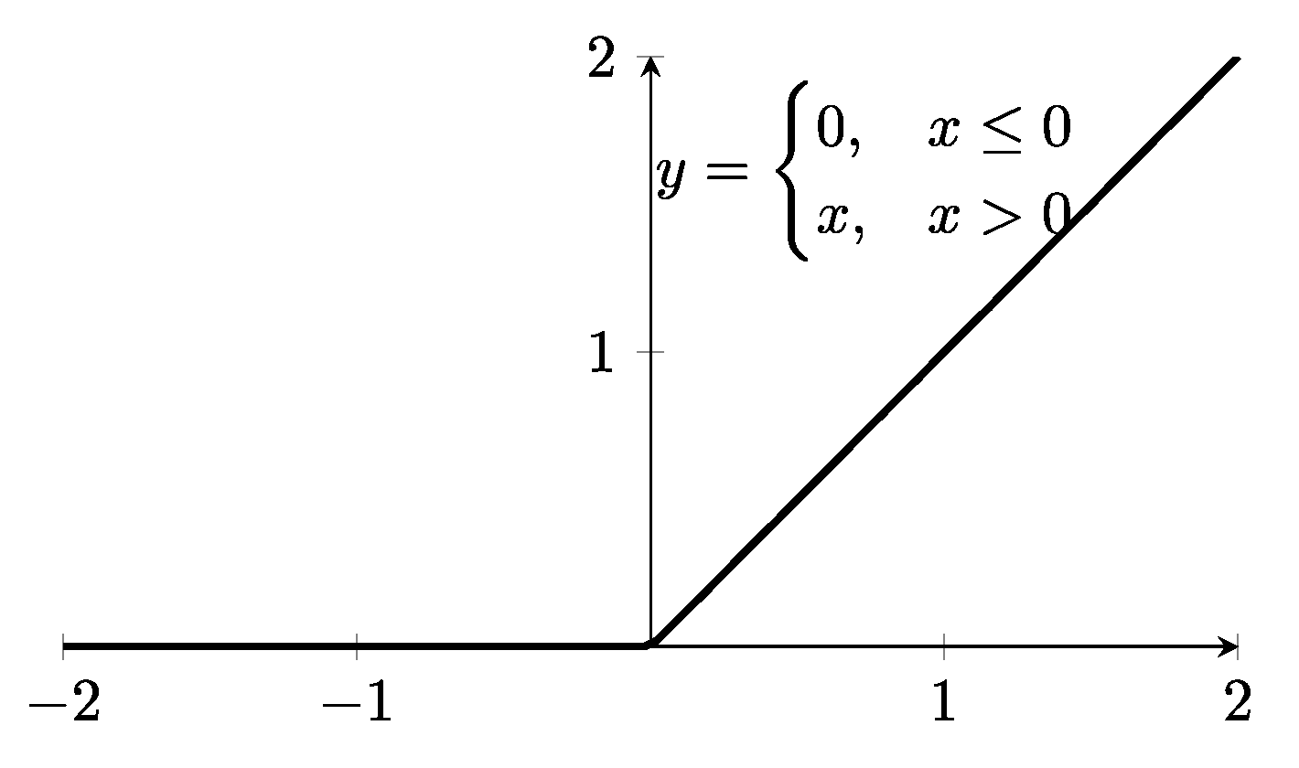
Figure 3.
Visual representation of the 1D-convolutional neural network structure used in this study.
Figure 3.
Visual representation of the 1D-convolutional neural network structure used in this study.

Figure 4.
Spatial distribution of housing rental prices in the Atlanta Metropolitan Area.
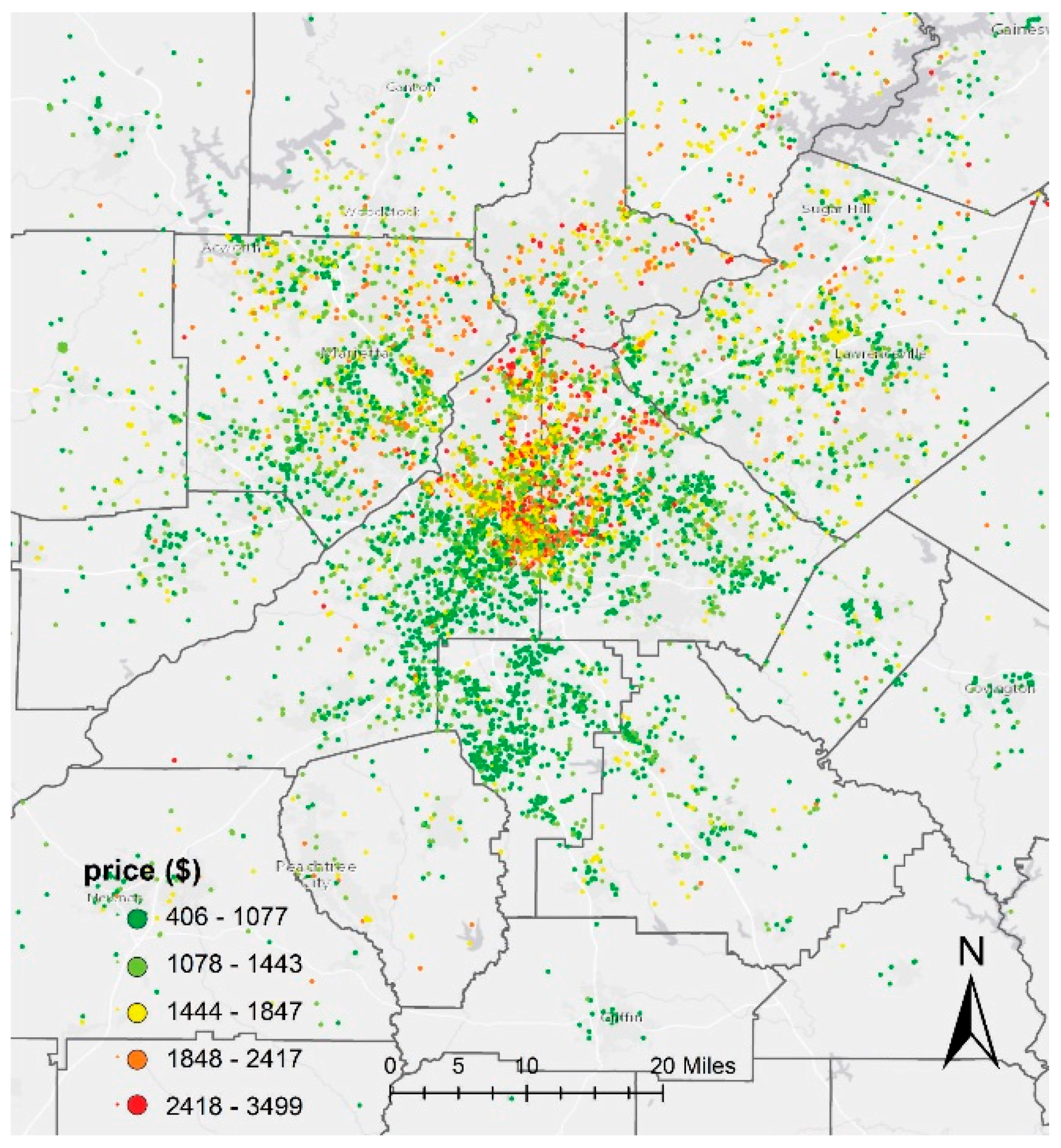
Figure 5.
Inputs, outputs, structural flows, and intermediate matrix dimensions of convolutional neural network (CNN) models. Each box represents a layer. Each layer has an input and an output. Within the parentheses in each box are the dimensions of the matrix.
Figure 5.
Inputs, outputs, structural flows, and intermediate matrix dimensions of convolutional neural network (CNN) models. Each box represents a layer. Each layer has an input and an output. Within the parentheses in each box are the dimensions of the matrix.

Figure 6.
Inputs, outputs, structural flows, and intermediate matrix dimensions of recurrent neural network (RNN) models. Each box represents a layer. Each layer has an input and an output. Within the parentheses in each box are the dimensions of the matrix.
Figure 6.
Inputs, outputs, structural flows, and intermediate matrix dimensions of recurrent neural network (RNN) models. Each box represents a layer. Each layer has an input and an output. Within the parentheses in each box are the dimensions of the matrix.


Table 1.
Descriptive statistics (price, bedroom number, and square footage) for the top ten counties (in terms of average prices) in the Atlanta Metropolitan Area.
Table 1.
Descriptive statistics (price, bedroom number, and square footage) for the top ten counties (in terms of average prices) in the Atlanta Metropolitan Area.
| Price ($) | Bedroom (#) | Square Footage | ||||||||
|---|---|---|---|---|---|---|---|---|---|---|
| County | Mean | Std | Median | Mean | Std | Median | Mean | Std | Median | Count |
| Clayton | 975.7 | 195.5 | 953.0 | 2.1 | 0.9 | 2 | 1114.0 | 338.5 | 1059.5 | 3728 |
| Rockdale | 1043.7 | 206.7 | 1000.0 | 2.1 | 0.9 | 2 | 1170.2 | 355.1 | 1156.0 | 853 |
| Coweta | 1099.0 | 242.6 | 1050.0 | 2.1 | 0.9 | 2 | 1176.3 | 367.5 | 1154.0 | 1046 |
| Henry | 1118.9 | 240.1 | 1074.0 | 2.1 | 0.9 | 2 | 1247.6 | 386.7 | 1204.0 | 2260 |
| Paulding | 1123.5 | 221.8 | 1106.0 | 2.2 | 1.0 | 2 | 1307.9 | 461.6 | 1210.0 | 1033 |
| Cherokee | 1205.5 | 254.3 | 1189.0 | 2.1 | 0.9 | 2 | 1217.4 | 385.4 | 1160.0 | 1321 |
| Cobb | 1217.4 | 322.4 | 1182.0 | 2.0 | 0.9 | 2 | 1133.9 | 404.8 | 1100.0 | 9722 |
| Gwinnett | 1238.0 | 312.5 | 1190.0 | 2.1 | 1.0 | 2 | 1266.1 | 476.6 | 1196.0 | 8873 |
| Dekalb | 1301.8 | 420.1 | 1243.0 | 1.8 | 0.8 | 2 | 1093.7 | 372.6 | 1072.0 | 14188 |
| Fulton | 1509.1 | 495.2 | 1433.0 | 1.7 | 0.8 | 2 | 1059.6 | 348.6 | 1046.0 | 30261 |
Table 2.
Interpolation results from inverse distance weighting (IDW) and kriging methods. IDW_{1,2,3} means IDW with 1st, 2nd, and 3rd order. KG_{ORD,UNIV} means ordinary and universal kriging. KG_FULL_VARIABLES means Gaussian process regression based on location, bedrooms, and square footage.
Table 2.
Interpolation results from inverse distance weighting (IDW) and kriging methods. IDW_{1,2,3} means IDW with 1st, 2nd, and 3rd order. KG_{ORD,UNIV} means ordinary and universal kriging. KG_FULL_VARIABLES means Gaussian process regression based on location, bedrooms, and square footage.
| idw_1 | idw_2 | idw_3 | kg_Ord | kg_Univ | kg_Full_Variables | |
|---|---|---|---|---|---|---|
| MAE | 264.702 | 284.214 | 293.514 | 256.261 | 255.491 | 219.004 |
| MAPE (%) | 20.742 | 22.072 | 22.658 | 20.172 | 20.138 | 17.749 |
| RMSE | 370.853 | 397.315 | 411.412 | 359.853 | 359.027 | 325.607 |
Table 3.
Performance metrics from models based on numeric predictors. RF: Random forest, BAG: Bagging, ET: Extra tree, KNN-{5,10}: 5(10) Nearest neighbors, GBM: Gradient boost regression, CART decision trees, ADA: Ada boost, MLP-20: neural network (20 hidden units).
Table 3.
Performance metrics from models based on numeric predictors. RF: Random forest, BAG: Bagging, ET: Extra tree, KNN-{5,10}: 5(10) Nearest neighbors, GBM: Gradient boost regression, CART decision trees, ADA: Ada boost, MLP-20: neural network (20 hidden units).
| Small Training | Large Training | |||||
|---|---|---|---|---|---|---|
| MAE | MAPE (%) | RMSE | MAE | MAPE (%) | RMSE | |
| RF | 194.925 | 15.846 | 300.877 | 151.587 | 12.425 | 255.293 |
| BAG | 194.767 | 15.849 | 301.457 | 151.237 | 12.402 | 255.191 |
| ET | 197.246 | 15.934 | 312.839 | 153.146 | 12.531 | 263.026 |
| KNN-5 | 223.442 | 18.196 | 334.660 | 175.726 | 14.499 | 287.57 |
| KNN-10 | 226.884 | 18.575 | 334.697 | 182.711 | 15.067 | 289.153 |
| GBM | 214.492 | 17.662 | 312.705 | 205.166 | 17.025 | 300.727 |
| CART | 245.931 | 19.389 | 393.507 | 180.132 | 14.407 | 323.132 |
| EXTRA | 254.196 | 20.137 | 411.971 | 182.634 | 14.619 | 326.941 |
| ADA | 281.724 | 24.656 | 369.236 | 250.227 | 21.551 | 344.863 |
| MLP-20 | 312.400 | 25.380 | 419.337 | 278.284 | 23.023 | 381.732 |
Table 4.
Performance metrics for models based on textual information. RNN: Recurrent neural network based on LSTM. CNN: 1D-convolutional neural network. LSA: Latent semantic analysis.
Table 4.
Performance metrics for models based on textual information. RNN: Recurrent neural network based on LSTM. CNN: 1D-convolutional neural network. LSA: Latent semantic analysis.
| MAE | MAPE (%) | RMSE | |
|---|---|---|---|
| LSTM | 196.760 | 15.452 | 288.370 |
| CNN | 208.886 | 17.030 | 300.103 |
| LSA | 211.701 | 15.655 | 311.688 |
Table 5.
Rental price predictions based on representative short descriptions.
| ShortDesc | Predicted Price |
|---|---|
| 1 BEDROOM APARTMENT AVAILABLE! | 1093.51 |
| 2 BEDROOM APARTMENT AVAILABLE! | 1210.22 |
| APARTMENTS WITH GOOD CONDITION FOR RENT | 1159.77 |
| LUXURY APARTMENTS FOR RENT, DO NOT MISS | 1318.34 |
| LUXURY APARTMENTS FOR RENT, CLOSE TO BUCKHEAD | 1351.13 |
Table 6.
Performance of models utilizing both numeric and textual information. RF: Random forest, BAG: Bagging, ET: Extra tree, KNN_{10,20}: 10(20) Nearest neighbors, GBM: Gradient boost regression, MLP-20: Neural network (20 hidden units), LR: Linear model, LASSO: Lasso regression, RIDGE: Ridge regression.
| MAE | MAPE (%) | RMSE | |
|---|---|---|---|
| bag | 145.358 | 11.703 | 227.967 |
| rf | 145.4 | 11.702 | 227.945 |
| et | 150.648 | 12.119 | 234.685 |
| gbm | 159.673 | 12.833 | 237.805 |
| knn-20 | 156.105 | 12.653 | 238.597 |
| knn-10 | 154.66 | 12.472 | 239.211 |
| mlp-20 | 172.668 | 13.859 | 254.023 |
| lr | 176.686 | 14.044 | 260.452 |
| lasso | 176.686 | 14.044 | 260.452 |
| ridge | 176.686 | 14.044 | 260.452 |
© 2019 by the authors. Licensee MDPI, Basel, Switzerland. This article is an open access article distributed under the terms and conditions of the Creative Commons Attribution (CC BY) license (http://creativecommons.org/licenses/by/4.0/).
Share and Cite
MDPI and ACS Style
Zhou, X.; Tong, W.; Li, D. Modeling Housing Rent in the Atlanta Metropolitan Area Using Textual Information and Deep Learning. ISPRS Int. J. Geo-Inf. 2019, 8, 349. https://0-doi-org.brum.beds.ac.uk/10.3390/ijgi8080349
AMA Style
Zhou X, Tong W, Li D. Modeling Housing Rent in the Atlanta Metropolitan Area Using Textual Information and Deep Learning. ISPRS International Journal of Geo-Information. 2019; 8(8):349. https://0-doi-org.brum.beds.ac.uk/10.3390/ijgi8080349
Chicago/Turabian StyleZhou, Xiaolu, Weitian Tong, and Dongying Li. 2019. "Modeling Housing Rent in the Atlanta Metropolitan Area Using Textual Information and Deep Learning" ISPRS International Journal of Geo-Information 8, no. 8: 349. https://0-doi-org.brum.beds.ac.uk/10.3390/ijgi8080349
Note that from the first issue of 2016, this journal uses article numbers instead of page numbers. See further details here.