Distributed Processing of Location-Based Aggregate Queries Using MapReduce

Department of Maritime Information and Technology, National Kaohsiung University of Science and Technology, 80543 Kaohsiung City, Taiwan
ISPRS Int. J. Geo-Inf. 2019, 8(9), 370; https://0-doi-org.brum.beds.ac.uk/10.3390/ijgi8090370
Submission received: 17 July 2019
/
Revised: 12 August 2019
/
Accepted: 19 August 2019
/
Published: 23 August 2019
(This article belongs to the Special Issue Distributed and Parallel Architectures for Spatial Data)
Abstract
:The location-based aggregate queries, consisting of the shortest average distance query (SAvgDQ), the shortest minimal distance query (SMinDQ), the shortest maximal distance query (SMaxDQ), and the shortest sum distance query (SSumDQ) are new types of location-based queries. Such queries can be used to provide the user with useful object information by considering both the spatial closeness of objects to the query object and the neighboring relationship between objects. Due to a large amount of location-based aggregate queries that need to be evaluated concurrently, the centralized processing system would suffer a heavy query load, leading eventually to poor performance. As a result, in this paper, we focus on developing the distributed processing technique to answer multiple location-based aggregate queries, based on the MapReduce platform. We first design a grid structure to manage information of objects by taking into account the storage balance, and then develop a distributed processing algorithm, namely the MapReduce-based aggregate query algorithm (MRAggQ algorithm), to efficiently process the location-based aggregate queries in a distributed manner. Extensive experiments using synthetic and real datasets are conducted to demonstrate the scalability and the efficiency of the proposed processing algorithm.
1. Introduction
With the fast advances of ubiquitous and mobile computing, processing the location-based queries on spatial objects [1,2,3,4,5,6] has become essential for various applications, such as traffic control systems, location-aware advertisements, and mobile information systems. Currently, most of the conventional location-based queries focus exclusively on a single type of objects (e.g., the nearest neighbor query finds a closest restaurant or hotel to the user). In other words, the different types of objects (termed the heterogeneous objects) are independently considered in processing the location-based queries, which means that the neighboring relationship between the heterogeneous objects is completely ignored. Let us consider a scenario where the user wants to stay in a hotel, have lunch in a restaurant, and go to the movies. Here, the hotel, the restaurant, and the theater refer to the heterogeneous objects. If the nearest neighbor queries are independently processed for the heterogeneous objects, the user is able to know his/her closest hotel, restaurant, and theater, which, however, may actually be far away from each other. Therefore, in addition to the spatial closeness of the heterogeneous objects to the query point, the neighboring relationship between the heterogeneous objects should also play an important role in determining the query result.
In the previous work [7], we present the location-based aggregate queries to provide information of the heterogeneous objects by taking into account both the neighboring relationship and the spatial closeness of the heterogeneous objects. In order to preserve the neighboring relationship between the heterogeneous objects, the location-based aggregate queries aim at finding the heterogeneous objects closer to each other by constraining their distance to be within a user-defined distance d. The set of objects satisfying the constraint of distance d is termed the heterogeneous neighboring object set (or HNO set). On the other hand, for maintaining the spatial closeness of the heterogeneous objects to the query point, four types of location-based aggregate queries are presented to provide information of HNO set according to specific user requirement. They are the shortest average-distance query (or SAvgDQ), the shortest minimal-distance query (or SMinDQ), the shortest maximal-distance query (or SMaxDQ), and the shortest sum-distance query (or SSumDQ), which are described respectively as follows.
- Consider the n types of objects, , , …, . Assume that there are mHNO sets, , , …, , where , , and . Given a query point q, a set of objects among these m HNO sets is determined, such that
- -
- for the SAvgDQ, the average distance of to q is equal towhere refers to the distance between objects and q.
- -
- for the SMinDQ, the distance of an object to q is equal to
- -
- for the SMaxDQ, the distance of an object to q is equal to
- -
- for the SSumDQ, the traveling distance from q to is equal towhere is the shortest distance that, starting from q, visits each object in exactly once.
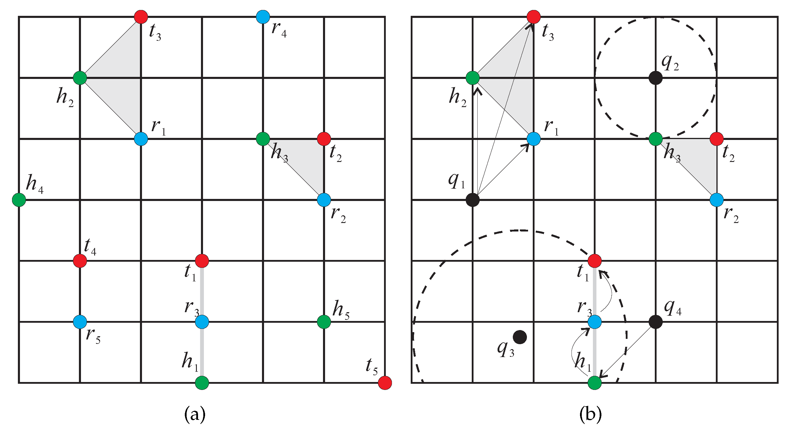
Let us use Figure 1 to illustrate how to process the four types of location-based aggregate queries (i.e., the SAvgDQ, the SMinDQ, the SMaxDQ, and the SSumDQ). As shown in Figure 1a, there are three types of data objects in the space, the hotels to , the restaurants to , and the theaters to . Assume that the user-defined distance d is set to 2 (that is, the distance between any two objects should be less than or equal to 2), which leads to three HNO sets, , , and (shown as the gray areas). Take the query point in Figure 1b, issuing the SAvgDQ, as an example. For each HNO set, the distance between each object in the HNO set and the query point needs to be first computed and then the HNO set with the shortest average-distance to is the result set of the SAvgDQ (i.e., the set ). Meanwhile, the SMinDQ and the SMaxDQ issued by the query points and , respectively, also need to be evaluated. When the SMinDQ is considered, the distances of the objects closest to in , , and , respectively, are compared to each other, and then the HNO set (i.e., ) containing ’s nearest neighbor is returned as the result set. In contrast to the SMinDQ, the SMaxDQ takes the furthest object in each HNO set into account. For the query point , its furthest objects in the three HNO sets are , , and , respectively. Among them, object has the shortest distance to , and hence the SMaxDQ retrieves the set because it contains . Consider the SSumDQ issued from the query point , which is processed simultaneously by the system. The shortest traveling path for each of the three HNO sets , , and has to be determined so as to find the HNO set resulting in a shortest traveling distance from . Finally, the set can be the SSumDQ result because of its shortest path .
The processing techniques developed in [7] focus only on efficiently processing a location-based aggregate query (corresponding to SAvgDQ, SMinDQ, SMaxDQ, or SSumDQ). However, in highly dynamic environments, where users can obtain object information through the portable computers (e.g., laptops, 3G mobile phones, and tablet PCs), multiple location-based aggregate queries must be issued by the users from anywhere and anytime (For instance, in Figure 1, the SAvgDQ, the SMinDQ, the SMaxDQ, and the SSumDQ are issued from different query points at the same time.) It means that, when there is a large number of location-based aggregate queries processed concurrently, the time spent on sequentially evaluating the location-based aggregate queries would dramatically increase. Even worse, at the time at which a location-based aggregate query terminates, the query result may already be outdated. As a result, it is necessary to design the distributed processing techniques to rapidly evaluate multiple location-based aggregate queries.
To achieve the objective of distributed processing of location-based aggregate queries, we adopt the most notable platform, MapReduce [8], for processing multiple queries over large-scale datasets by involving a number of share-nothing machines. For data storage, an existing distributed file system (DFS), such as Google File System (GFS) or Hadoop Distributed File System (HDFS), is usually used as the underlying storage system. Based on the partitioning strategy used in the DFS, data are divided into equal-sized chunks, which are distributed over the machines. For query processing, the MapReduce-based algorithm executes in several jobs, each of which has three phases: map, shuffle, and reduce. In the map phase, each participating machine prepares information to be delivered to other machines. As for the shuffle phase, it is responsible for the actual data transfer. In the reduce phase, each machine performs calculation using its local storage. The current job finishes after the reduce phase. If the process has not been completed, another MapReduce job starts. Depending on the applications, the MapReduce job may be executed once or multiple times.
In this paper, we focus on developing the MapReduce-based methods to efficiently answer multiple location-based aggregate queries (consisting of numerous SAvgDQ, SMinDQ, SMaxDQ, and SSumDQ issued concurrently from different query points) in a distributed manner. We first utilize a grid structure to manage the heterogeneous objects in the space by taking into account the storage balance, and information of the partitioned object data in each grid cell is stored in the DFS. Next, we propose a distributed processing algorithm, namely the MapReduce-based aggregate query algorithm (MRAggQ algorithm for short), which is composed of four phases: the Inner HNO set determining phase, the Outer HNO set determining phase, the Aggregate-distance computing phase, and the Result set generating phase, each of which executes a MapReduce job to finish the procedure. Finally, we conduct a comprehensive set of experiments over synthetic and real datasets, demonstrating the efficiency, the robustness, and the scalability of the proposed MRAggQ algorithm, in terms of the average running time in performing different workloads of location-based aggregate queries.
The rest of this paper is organized as follows. In Section 2, we review the previous work on processing various types of location-based queries in centralized and distributed environments. Section 3 describes the grid structure used for maintaining information of the heterogeneous objects. In Section 4, we present how the MRAggQ algorithm can be used to process multiple location-based aggregate queries efficiently. Section 5 shows extensive experiments on the performance of the proposed methods. In Section 6, we conclude the paper with directions on future work.
2. Related Works
Efficient processing of the location-based queries is an emerging research topic in recent years. Here, we first review the centralized methods for processing the location-based queries on a single object type and multiple types of objects (i.e., the heterogeneous objects). Then, we discuss the MapReduce programming technique and survey some works on processing the location-based queries using MapReduce.
2.1. Centralized Processing Techniques for Location-Based Queries
Most of the conventional location-based queries on a single data type concentrate on discovering the spatial closeness of objects to the query object. The range query [9,10] is a well-known query, used to find a set of objects that are inside a spatial region specified by the user. If the spatial region is constructed according to the location of the query object q, another variation of range query, the within query [11,12], is presented to find the objects whose distances to q are less than or equal to a user-given distance d (i.e., finding the objects within the region centered at q with radius d). Recently, many efforts have been made on processing the range and within queries in different research domains, such as mobile information systems [3,13] and uncertain database systems [2,14]. The nearest neighbor query [15,16] is the most common type of location-based queries, as it has important applications to the provision of location-based services. Many variations of nearest neighbor query have been proposed in numerous applications. To address the issue of scalability, the KNN join query [17,18] is presented to find the K-nearest neighbors for all objects in a query set. To express requests by groups of users, the aggregate nearest neighbor (ANN) query (a.k.a. group nearest neighbor query) is proposed by Papadias et al. [19]. Given a set of query objects Q and a set of objects O, ANN query returns the object in O minimizing an aggregate distance function (e.g., sum or max) with respect to the objects in Q. A variation of nearest neighbor query with asymmetric property is the reverse nearest neighbor (RNN) query [1]. Given the query object q, the RNN query retrieves the set of objects whose nearest neighbor is q. The skyline query, also known as the maximal vector problem [20,21], is first studied in the area of computational geometry. Then, Borzsonyi et al. [22] introduce the skyline operator into database systems. If an object is not dominated by any other objects in terms of multiple attributes, then it is a skyline point. By taking into account the object locations, the spatial skyline query [4] is proposed, where the distance of objects plays an important role in determining the skyline points. Given a set of m query objects and a set of n data objects, each data object has m attributes, each of which refers to its distance to a query object. The spatial skyline query retrieves the skyline points that are not dominated in terms of the m attributes.
Some related work on processing the location-based queries tries to keep the neighboring relationship between the heterogeneous objects. Given two types of data objects A and B, the K closest pair query [23] finds the K closest object pairs between A and B (that is, the K pairs , where and , with the smallest distance between them). Another type of location-based queries on the two data sources is the spatial join query [24], which maintains a set of object pairs (each pair has one item from the two data sources respectively) satisfying a given spatial predicate (e.g., overlap or coverage). Papadias et al. [25] further extend the spatial join query to the multiway spatial join query, in which the spatial predicate is a function over m data sources (where ). Zhang et al. [26] present the KNG query to determine the query result based on (1) the minimum distance between the heterogeneous objects and the query object (referred to as inter-group distance) and (2) the maximum distance among the heterogeneous objects (referred to as inner-group distance). Given a spatial database with m types of data objects and a query object q, the KNG query returns the K groups (each of which consists of one object from each data type) with the minimum sum of the inner-group distance and the inter-group distance. However, due to the fact that the KNG query considers the sum of inner-group and inter-group distances, the object group retrieved by executing the KNG query is likely to be close to the query object but far away from each other (i.e., the inter-group distance dominates the query result), or close to each other but far away from the query object (i.e., the inner-group distance affects the result). To appropriately keep the spatial closeness and the neighboring relationship of objects, in our previous work [7], the location-based aggregate queries are presented to obtain information of the NHO sets.
2.2. Distributed Processing Techniques for Location-Based Queries
As mentioned in Section 1, MapReduce is a popular programming framework, which can be used to support the distributed processing of location-based queries. A MapReduce algorithm proceeds in several jobs, each of which has the map, the shuffle, and the reduce phases. In the map phase, for each participating machine, a list of key-value pairs is generated from its local storage, where the key k is usually numeric and the value v corresponds to arbitrary information. According to the key k, each pair is transmitted to another machine in the shuffle phase. More specifically, the shuffle phase distributes the key-value pairs across the machines following the rule that pairs with the same key are delivered to the same machine. In the reduce phase, each machine incorporates the key-value pairs received form the shuffle phase into its local storage, and performs the task using the local data. When the reduce phases of all machines are completed, the current MapReduce job terminates.
There has been considerable interest on supporting location-based queries over MapReduce framework. Cary et al. [27] present the techniques for building R-trees based on MapReduce, which, however, do not address the issues of processing the location-based queries. Zhang et al. [28] show how the location-based queries can be naturally expressed in MapReduce framework, including the spatial selection queries, the spatial join queries, and the nearest neighbor queries. Ji et al. [29] propose a MapReduce-based approach, in which an inverted grid structure is built to index data objects, to answer the KNN queries. Furthermore, in [30], they extend their approach to process a variant of KNN queries, the RKNN query. Akdogan et al. [31] focus on processing various types of location-based queries (including RNN, MaxRNN, and KNN queries), by creating a Voronoi diagram based on the MapReduce programming model for data objects. In their method, each data object is represented as a pivot which is then used to partition the space. Yokoyama et al. [32] propose a method that decomposes the given space into cells and evaluates the AKNN queries using MapReduce in a distributed and parallel manner. Zhang et al. [33] present the exact and approximate MapReduce-based algorithms to efficiently perform parallel KNN join queries on a large-scale dataset. To improve the performance of KNN join queries, Lu et al. [34] further design an effective mapping mechanism, by exploiting pruning rules for distance filtering, to reduce both the shuffling and computational costs.
Recently, Eldawy et al. [35,36] focus on developing a MapReduce framework, the SpatialHadoop, which is a comprehensive extension of Hadoop. The SpatialHadoop provides an expressive high level language for spatial objects, adapts a set of spatial index structures (e.g., Grid structure, R-tree, and R-tree) which is built-in HDFS, and supports the traditional location-based queries (including the range, KNN, and spatial join queries). Moreover, in [37], they address the issue of processing the skewed distributed datasets in the SpatialHadoop, by presenting a box counting function to detect the degree of skewness of a spatial dataset. The SpatialHadoop is carefully designed for the location-based queries, in which the spatial closeness of a single type of objects to the query point is a main concern in determining the query result. However, it cannot directly be applied for answering the location-based aggregate queries because (1) the query result consists of the heterogeneous objects, rather than a single type of objects, and (2) whether the heterogeneous objects satisfy the constraint of distance d (i.e., with the better neighboring relationship) should be taken into account.
3. Grid Structure
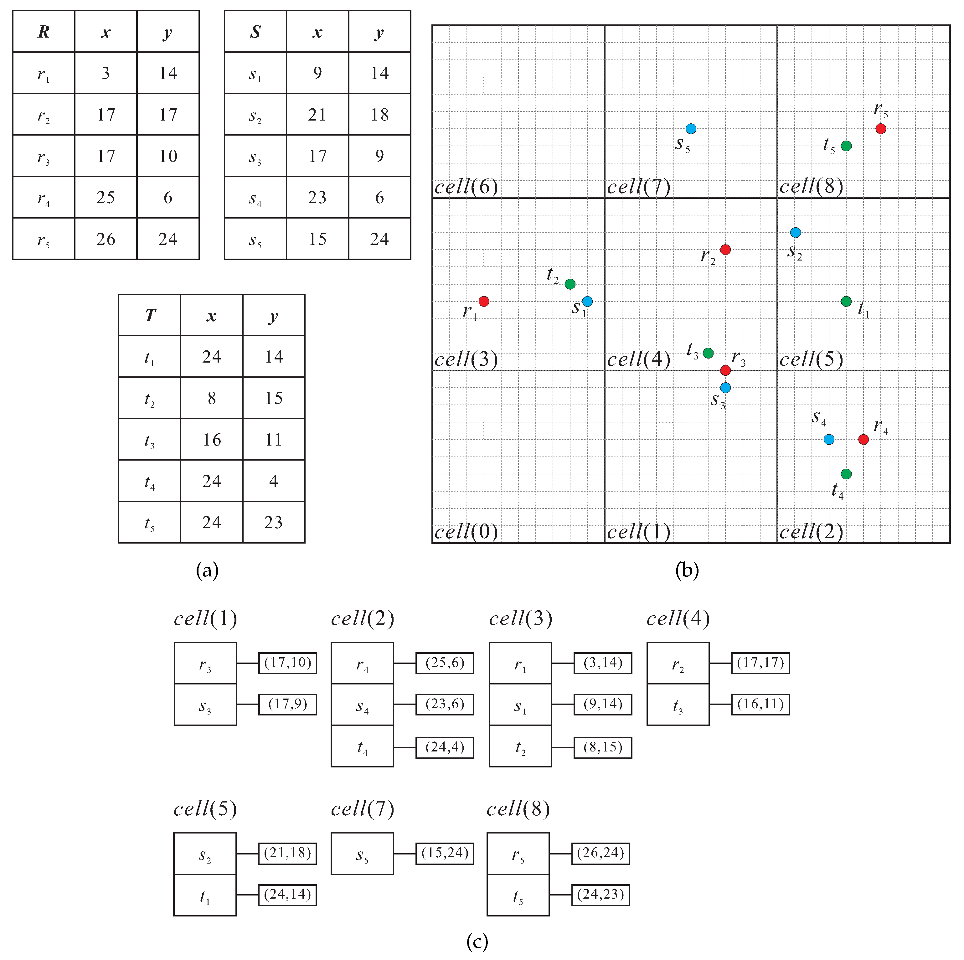
In our model, there are n types of data objects (i.e., the heterogeneous objects) in the space. As the location database contains large amounts of information that need to be maintained, a grid structure is used to manage such information by partitioning the space into multiple gird cells, each of which stores data of objects enclosed in it. In order to balance the storage load of each grid cell, the data space is partitioned into equal-sized cells by considering a pre-defined parameter . Initially, all the heterogeneous objects are grouped into cells. Then, the number of objects enclosed in a cell is compared with the parameter . Once the object number is greater than , the data space covering all objects is repartitioned into cells. Similarly, if there still exists a cell within which the object number exceeds , then the data space needs to be repartitioned into cells. This partitioning process continues until each cell satisfies the condition that the number of objects in is less than or equal to . By exploiting the parameter , the storage overhead for maintaining information of objects can be evenly distributed among the cells. Figure 2 shows an example of how the data space is divided by taking into account the storage load of each cell. As shown in Figure 2a, there are three types of data objects, R, S, and T in the space, each of which has five objects with coordinate (e.g., object ’s coordinate refers to ). Suppose that the pre-defined parameter is set to 3. The data space would be divided into cells, so as to guarantee that the number of objects in each cell does not exceed 3. The final divided grid cells, which are numbered from 0 to 8, are shown in Figure 2b.
In order to provide parallel processing of the heterogeneous objects using MapReduce, information of the grid structure is stored in a distributed storage system, the HDFS, by default. The HDFS consists of multiple DataNodes for storing data and a NameNode for monitoring all DataNodes. In the HDFS, a file is broken into multiple equal-sized chunks and then the NameNode allocates the data chunks among the DataNodes for query processing. Returning to the example in Figure 2, the cells, to , are treated as the chunks and kept on the HDFS. Take the cell as an example, as objects and are enclosed in , in the HDFS, the chunks with respect to will store and with their coordinates and , respectively. Note that the cells and need not be kept on the HDFS because there is no object in them. Figure 2c shows how the grid structure for the heterogeneous objects is stored on the HDFS.
4. Mapreduce-Based Aggregate Query Algorithm
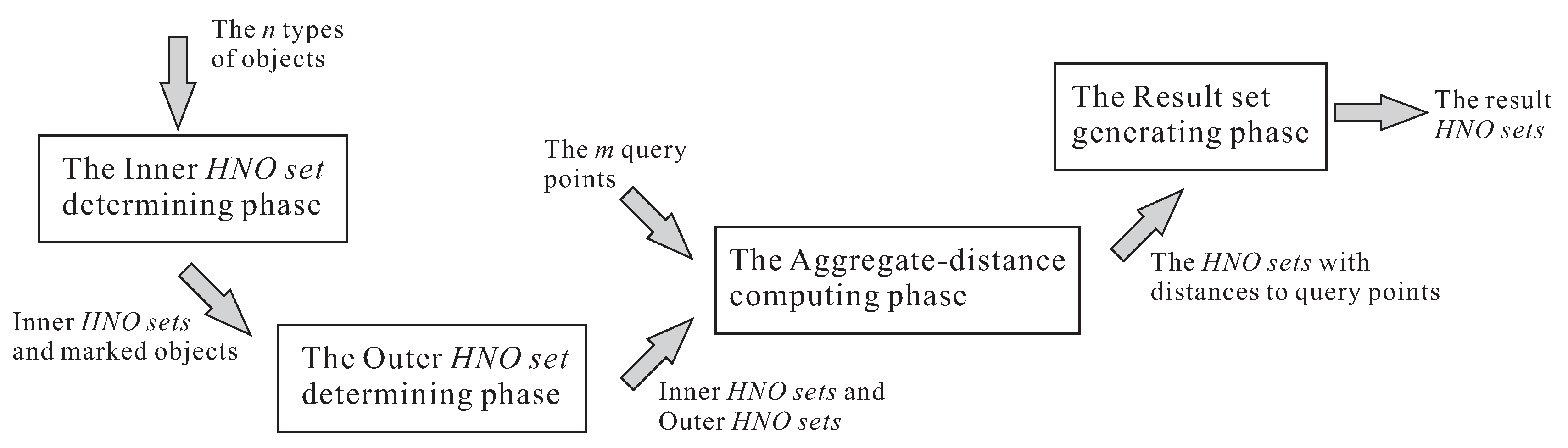
Given the n types of data objects, , , …, , a set of query points Q (where a query point corresponds to a SAvgDQ, a SMinDQ, a SMaxDQ, or a SSumDQ), and the user-defined distance d, the main goal of the MapReduce-based aggregate query (MRAggQ) algorithm is to efficiently determine, for each query point q, the HNO set with the shortest distance in a distributed manner. Recall that a set of objects (where and ) can be included in the result set of the location-based aggregate queries only if the following two conditions hold: (1) the distance between any two objects in is less than or equal to d (as a necessary condition) and (2) has the shortest average, minimal, maximal, or sum distance to the query point. As a result, the MRAggQ algorithm is developed according to the two conditions. The proposed MRAggQ algorithm consists of four phases, in which the first and last two phases are in charge of checking the conditions (1) and (2), respectively. In the following, we briefly describe the purposes of the four phases and then discuss the details separately. To provide an overview of the MRAggQ algorithm, a flowchart and a pseudo code for the four phases are also given in Figure 3 and Algorithm 1, respectively:
- The first phase, the Inner HNO set determining phase, aims at finding, for each cell , the sets of objects that are enclosed in and are within the distance d from each other. Here, we term the object sets found in this phase the Inner HNO sets.
- The second phase, the Outer HNO set determining phase, focuses on finding the HNO sets that have not been discovered from the previous phase. It means that the objects constituting a HNO set determined in this phase cannot be fully enclosed in a cell. Instead, the objects are distributed over different cells. We term the HNO sets discovered in this phase the Outer HNO sets.
- The third phase, the Aggregate-distance computing phase, is responsible for computing the aggregate-distances of all HNO sets obtained from the previous two phases to each query point contained in the query set Q, according to the type of location-based aggregate queries (i.e., the aggregate-distance may be the average, the minimal, the maximal, or the sum distance).
- The last phase, the Result set generating phase, sorts the aggregate-distances of all HNO sets computed in the previous phase, so as to output the HNO set with the shortest aggregate-distance for each query point in Q.
| Algorithm 1: The MRAggQ algorithm | |
| Input: The n types of objects, and the set of m query points | |
| Output: The result HNO set for each query point | |
| /* The Inner HNO set determining phase | */ |
| finding the Inner HNO sets enclosed in ; | |
| determining the marked objects for ; | |
| /* The Outer HNO set determining phase | */ |
| finding the Outer HNO sets based on the marked objects; | |
| combing the Inner and the Outer HNO sets; | |
| /* The Aggregate-distance computing phase | */ |
| computing the average, min, max, or sum distances of the HNO sets to the m query points; | |
| /* The Result set generating phase | */ |
| sorting the HNO sets according to their distances to each query point; | |
| returning the HNO set with the shortest distance to each query point; | |
4.1. Inner HNO Set Determining Phase
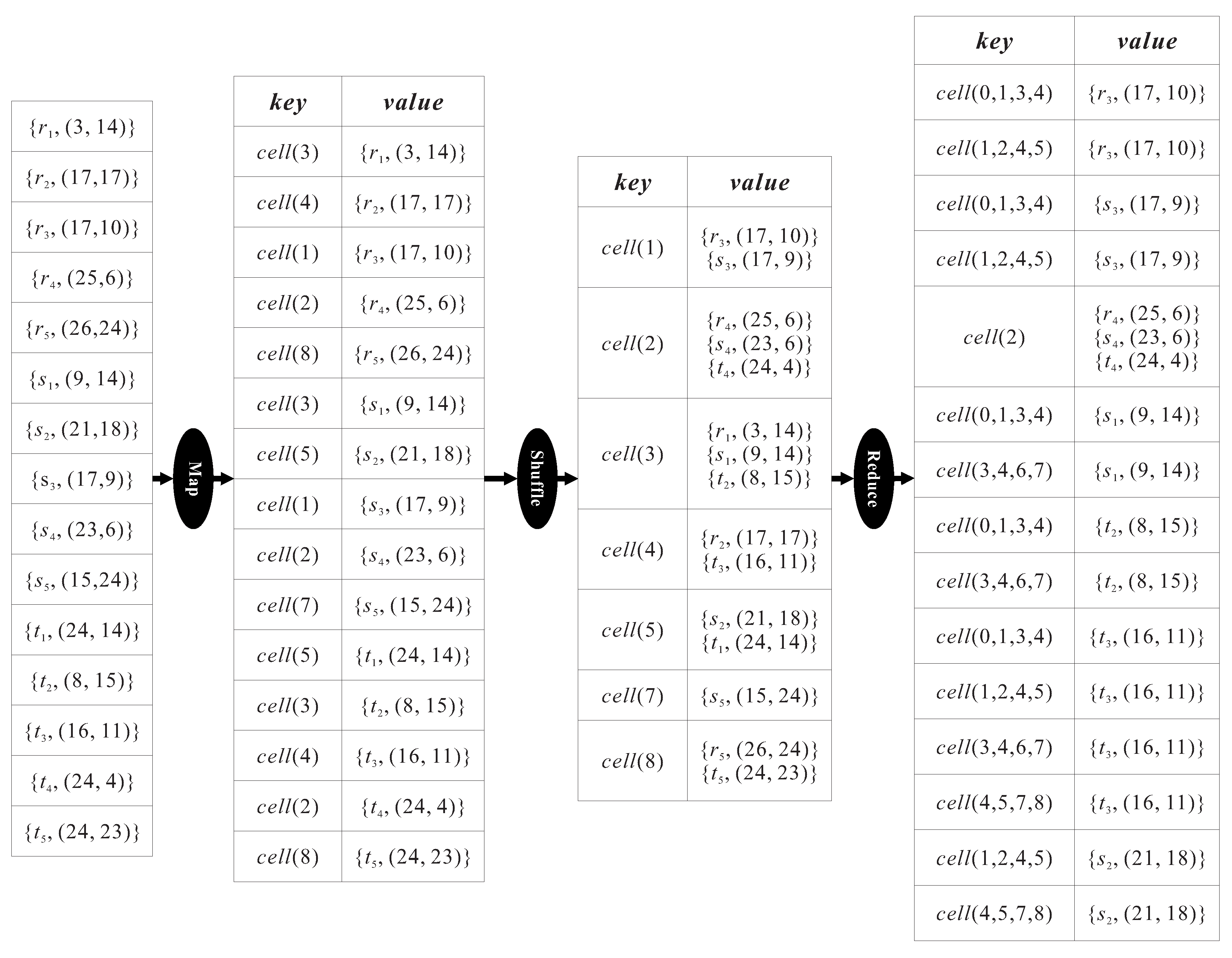
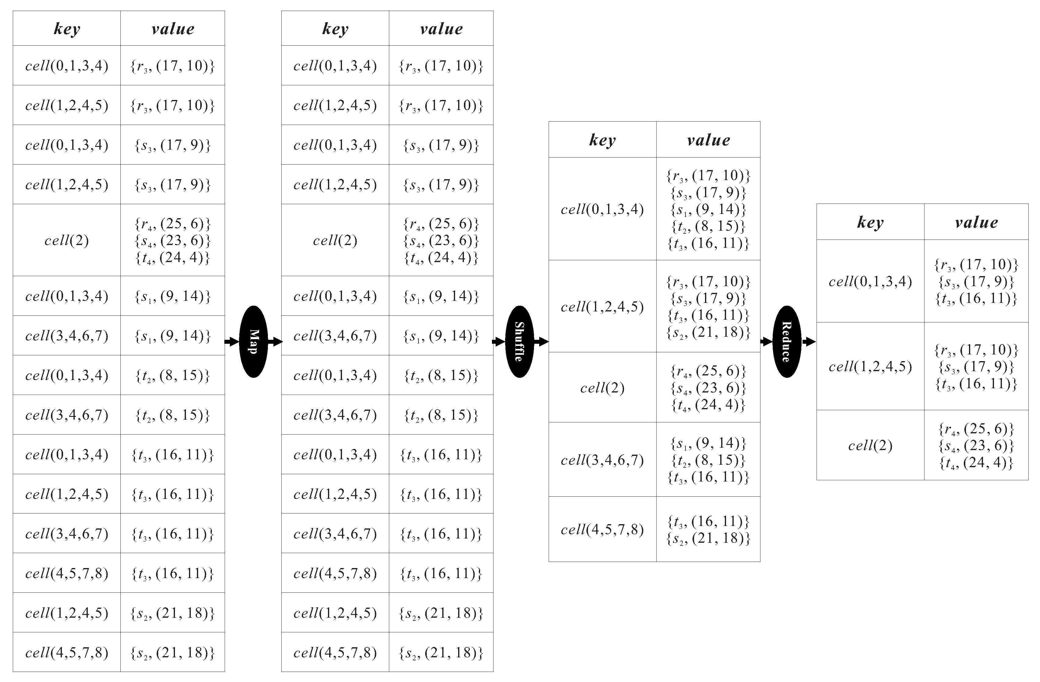
Given the n types of objects stored on the HDFS, the goal of the Inner HNO set determining phase is to process in parallel, determining the Inner HNO sets for each cell , each of which is composed of n types of objects enclosed in . In this phase, a MapReduce job consisting of the map step, the shuffle step, and the reduce step is executed to finish the procedure. In the map step, each cell in the form of (i.e., pair) is extracted from the HDFS as input. The pair generated by the map step is then transmitted to another machine in the shuffle step, where the recipient machine is determined solely by value of . That is, if the pairs have a common key , all of them will arrive at an identical machine for processing in the reduce step. This is because for the n pairs (where ) with the same key , a set composed of the n objects , , …, has a chance to be the Inner HNO set as all the objects are enclosed in the cell . In the reduce step, two processing tasks are carried out in each participating machine, by taking into account the key-value pairs received from the shuffle step.
- The first task is to compute the distance between any two objects and enclosed in , where and , based on their coordinates and . Consider a set of objects enclosed in the cell . If the computed distances of all object pairs are less than or equal to the distance d, then is an Inner HNO set of . Hence, a key-value pair in the form of , is returned as output.
- The second task, as a preliminary to the next phase, the Outer HNO set determining phase, focuses on marking some objects enclosed in cell that may constitute an Outer HNO set with the other objects enclosed in different cells. We term the objects determined by the second task the marked objects. For an object enclosed in , it can be the marked object only if the circle centered at with radius d is not fully contained in . Otherwise (i.e., the circle is enclosed by ), there exists no object enclosed in another cell and whose distance to object is less than or equal to d, and thus must not be contained in the Outer HNO sets. Suppose that the data space is divided into cells, where each equal-sized cell is represented as a rectangle with widths and on the x-axis and y-axis, respectively. An object with coordinates is a marked object in cell if the following condition holds:Similar to the first task, a key-value pair with respect to each marked object (i.e., ) will be generated after executing the second task. The generated key is mainly used to guarantee that the n types of objects constituting an Outer HNO set can be processed in the same machine. Note that, if such objects are considered in different machines, some of the Outer HNO sets may be lost. In order to give each marked object enclosed in the cell a key , we first merge cells into a rectangle R bounding the cell , where the parameters and are estimated based on the following equation:Then, the key of the marked object is set to the union of the ids of these cells. To establish better understanding of the main idea behind Equation (2), we take the cell in Figure 2b as an example, where the user-defined distance and both the widths and of each cell are equal to 10. Based on Equation (2), a rectangle R consisting of cells is constructed to enclose the cell (here, R can be represented as , , , and ). Let us consider the rectangle R corresponding to . As the minimal distance between and each of the other three cells, , , and is less than or equal to d, it is possible that an Outer HNO set is composed of one or more marked objects in and the rest in the other three cells. As such, we should give all the marked objects enclosed in the rectangle R a common key, , so as to process them in the same machine. In addition, the keys , , and are assigned to the marked objects enclosed in their corresponding rectangle R in the same way.
Figure 4 is a concrete example, which continues the previous example in Figure 2, illustrating the data flow of the MapReduce job for the Inner HNO set determining phase. In the map step, a key for each object is extracted and transformed into key-value pair, (e.g., for the object ). Then, the key-value pairs with the same key are shuffled to the same machine for processing. For example, and arrive at the same machine because of their common key . In the reduce step, each participating machine carries out the first task (i.e., determining the Inner HNO sets) by computing the distance between objects received from the shuffle step to compare with the distance . In this figure, , is output, so that is an Inner HNO set enclosed in the cell . Meanwhile, the second task (i.e., finding the marked objects) is executed in each machine to find the marked objects enclosed in a cell based on Equation (1) and give each marked object a key according to Equation (2). Take the marked object enclosed in the cell as an example. Four key-value pairs, , , , , and , will be output from the machine in charge of , as there is a chance that constitutes an Outer HNO set with the other marked objects enclosed in its surrounding cells. Finally, the Inner HNO sets and the marked objects with respect to each cell, discovered in the Inner HNO set determining phase, are passed to the next phase.
4.2. Outer HNO Set Determining Phase
The Outer HNO set determining phase focuses on finding the HNO sets that have not been discovered (i.e., the Outer HNO sets), by exploiting information of the marked objects obtained from the previous phase. Similarly, a MapReduce job is applied in the Outer HNO set determining phase, where (1) the map step receives the result of the previous phase and the key-value pairs are emitted, (2) the shuffle step dispatches the pairs with the same key to an identical machine for checking whether the Outer HNO sets exist, and (3) the reduce step computes the distance between the marked objects to compare with the distance d. Having executed the Outer HNO set determining phase, each key-value pair in the form of , is returned as output, where c refers to either a cell id (meaning that , is an Inner HNO set) or multiple cell ids (that is, an Outer HNO set). Continuing the example in Figure 4, the key-value pairs corresponding to an Inner HNO set, , , and the marked objects, and so on, are emitted in the map step of the Outer HNO set determining phase, as shown in Figure 5. In the shuffle step, the marked objects with the common key are assigned to the same machine for computing the distance between any two marked objects based on their coordinates. For instance, five marked objects , , , , and with the key will be considered in the same machine. In the reduce step, each participating machine computes the distance between the marked objects assigned by the shuffle step (note that only the distances between different types of marked objects are computed), and then outputs the Outer HNO sets. In this figure, the key-value pairs, and , are returned as they satisfy the constraint of distance d. As we can see, is a duplicate set and needs to be eliminated. The duplicate elimination will be carried out in the last phase, the Result set generating phase.
4.3. Aggregate-Distance Computing Phase
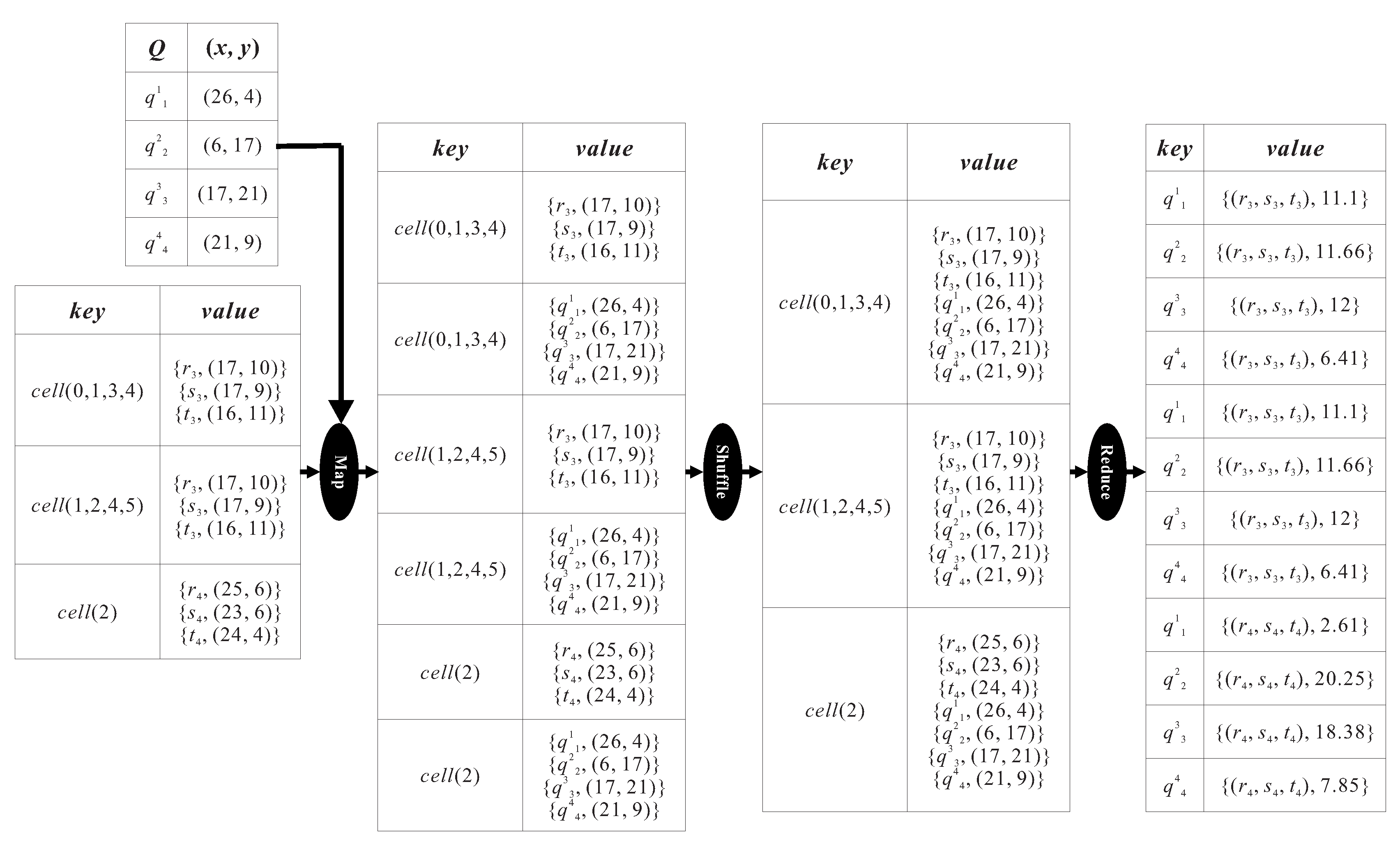
After executing the first two phases (i.e., the Inner HNO set determining phase and the Outer HNO set determining phase), all of the HNO sets in the space can be discovered in a distributed manner. In the sequel, the third phase, the Aggregate-distance computing phase, is designed to compute in parallel the aggregate-distance of each HNO set according to the type of location-based aggregate queries. Suppose that Q is a set of m query points, , , …, , at which a SAvgDQ, a SMinDQ, a SMaxDQ, or a SSumDQ is issued. A query table with respect to Q needs to be broadcast to each machine so as to estimate the aggregate-distances between the HNO sets processed by this machine and each query point in Q. Each tuple of the query table has two fields: the query id (where j can be 1, 2, 3, and 4, indicating SAvgDQ, SMinDQ, SMaxDQ, and SSumDQ, respectively) and the coordinates . In the map step of the Aggregate-distance computing phase, in addition to the key-value pair , for each HNO set, a key-value pair , , …, with regard to the query points is also emitted, so that the query set Q can be transmitted along with each HNO set to the same machine for query processing. Having executed the shuffle step, the HNO set and the query set with the same key are grouped together. For each participating machine, the task of computing the aggregate-distance between each HNO set and each query point assigned by the shuffle step is carried out in the reduce step, in which the aggregate-distance refers to the average, minimal, maximal, or sum distance according to the query type (i.e., the value of j). Finally, each key-value pair in the form of is returned as output, where is the aggregate-distance between the HNO set and the query point .
As shown in Figure 6, continuing the example of Figure 5, the query table maintains four query points to with their coordinates and query types, in which , , , and issue the SAvgDQ, the SMinDQ, the SMaxDQ, and the SSumDQ, respectively. In the map step, the key-value pairs , , , , and , , , obtained from the previous phase (i.e., the Outer HNO set determining phase) are emitted. For the sake of grouping the HNO sets and the query points, the key-value pairs, , , and so on, are also generated based on the keys , , and . The shuffle step dispatches the pairs with the same key to the same machine for computing the aggregate-distance between the HNO sets and the query points. Take the key-value pair with regard to the key as an example. The machine in charge of runs the reduce step to compute the average distance of the HNO set to the query point as the query type . Then, a key-value pair is output, meaning that the average distance is equal to . Similarly, in the reduce step, the min, max, and sum distances of to , , and , are estimated as , 12, and , respectively. After the key-value pairs have been output by all the participating machines, the last phase, the Result set generating phase, will sort the HNO sets in ascending order of their aggregate-distance to determine the query result.
4.4. Result Set Generating Phase
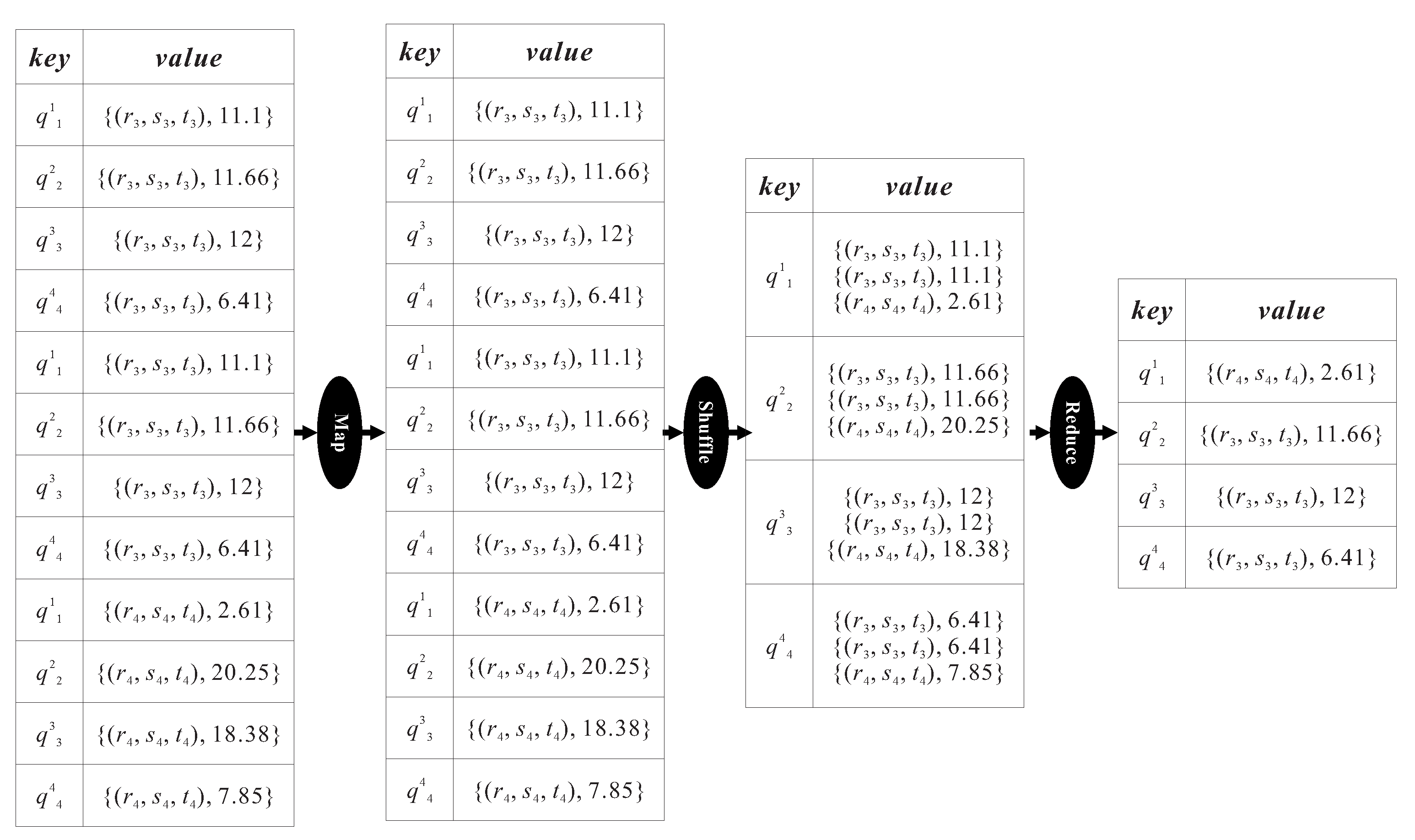
The goal of the last phase, the Result set generating phase, is to determine the HNO set with the shortest aggregate-distance for each query point in a distributed manner. Once a MapReduce job starts, the key-value pairs received from the previous phase are directly emitted in the map step. According to the key , the HNO sets having the same will be assigned to an identical machine in the shuffle step because their aggregate-distances to the query point need to be compared so as to determine the query result for . For the machine receiving the key-value pairs with respect to , the first task of the reduce step is to eliminate the duplicate value in the form of . Then, the second task is to sort the HNO sets in ascending order of their aggregate-distance , and finally output the HNO set with smallest as the query result.
Figure 7 gives an illustration of how the Result set generating phase is executed using the key-value pairs generated from the previous phase (shown in Figure 6). In the map step, all key-value pairs which use the query id as the key (e.g., ) are emitted so that the pairs with the same key can be grouped together for processing after the shuffle step. For instance, the pairs and are assigned to the same machine because of their common key . By executing the reduce step in each machine, the duplicates are first removed and then the HNO set with the shortest aggregate-distance for each query point is output. In this figure, the HNO set is the result for the query point , and the HNO set is the result for the other three query points , , and .
5. Performance Evaluation
In this section, we conduct a series of experiments to evaluate the performance of the proposed MRAggQ algorithm. We first study the effect of the used grid structure on the performance of processing the location-based aggregate queries, so as to decide an appropriate number of heterogeneous objects enclosed in each cell for query processing. Then, we demonstrate the efficiency and the scalability of the proposed MRAggQ algorithm by measuring its running time with respect to various important factors.
5.1. Performance Settings
All of the experiments are performed on a cluster of four computing machines. Each computing machine is a PC with Intel 2.70 GHz CPU and 16 GB RAM, and runs 32-bit Ubuntu 15.10. The algorithms are implemented in JAVA and allocate 4 GB RAM to the Java Virtual Machine. The computing machines are connected by a 1000 Mbps Ethernet and Hadoop 2.6.0 is used as the default distributed file system. One synthetic dataset and four real datasets are evaluated in our simulation. The synthetic dataset consists of n types of objects, where n varies from 1 to 5, and the total number of objects ranges from 1000 K to 5000 K. The objects are spread over a region of 1,000,000 × 1,000,000 with the Uniform distribution. As for the real datasets, we consider the Beijing, Manchester, Pittsburgh, and Charlotte files (containing about 400 K, 1000 K, 1200 K, and 1500 K objects, respectively) extracted from the OpenStreetMap [38]. The data space is divided into multiple cells by considering the parameter (i.e., the maximum number of objects enclosed in a cell), which varies from 250 to 2000 in the experiments, and then a grid structure is built to manage the heterogeneous objects enclosed in the cells. In the experimental space, we also generate a set of m query points (where m varies from K to 10 K). Each of the query points issues a SAvgDQ, a SMinDQ, a SMaxDQ, or a SSumDQ to the server, where the user-defined distance d ranges from to of the width of the cell.
The performance of the MRAggQ algorithm is measured by the average running time in performing workloads of the location-based aggregate queries issued from the m query points. We investigate the effects of five important factors on the performance of processing the location-based aggregate queries, including the parameter α (used for the grid index), the number of objects, the number of object types (i.e., n), the user-defined distance d, and the number of query points. Table 1 summarizes the parameters under investigation, along with their default values and ranges. In the sequel, we show the experimental results with detailed discussions for these important factors, respectively.
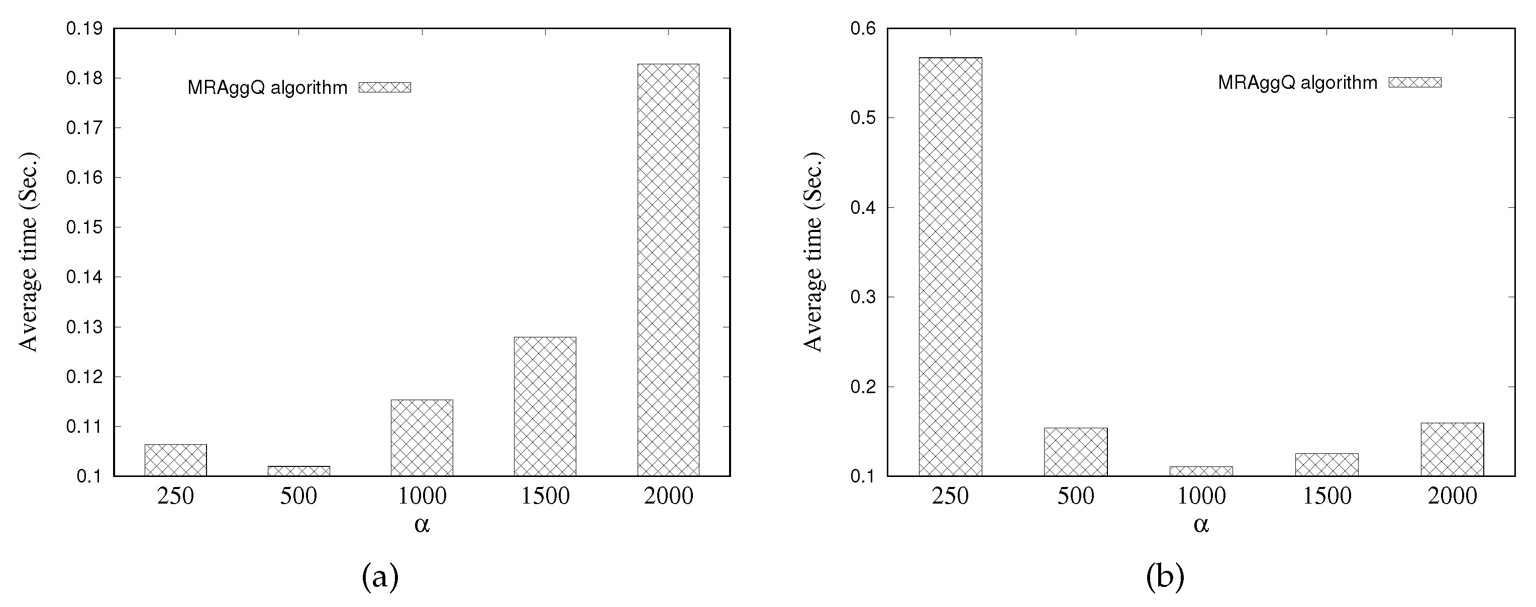
5.2. Effect of Parameter
The first set of experiments studies the effect of the number of objects enclosed in each cell (i.e., the parameter ) on the performance of processing the location-based aggregate queries, using the Uniform dataset and the Manchester dataset. In the experiments, we vary the value of the parameter from 250 to 2000 and evaluate the average running time for the proposed MRAggQ algorithm. For both the Uniform dataset and the Manchester dataset, the average running time first decreases and then increases with the increasing value of , as shown in Figure 8a,b, respectively. This is mainly because (1) for a smaller (i.e., fewer number of objects in each cell), more cells need to be generated for storing object information, and thus each participating machine (i.e., the DataNode) spends more time on processing the increasing number of cells assigned by the NameNode, while (2) for a greater (meaning that the number of cells decreases but the storage overhead for each cell increases), computing the distances between objects to determine the Inner and the Outer HNO sets with respect to each cell takes more processing time. As the parameter dominates the performance of processing the location-based aggregate queries, we need to decide an appropriate value of used to partition the data space. As we can see, for both the Uniform dataset and the Manchester dataset, the average running time increases noticeably after . The experimental result shows that is a better choice than the others, and hence will be used as the default value in all the rest experiments.
5.3. Effect of Number Of Objects
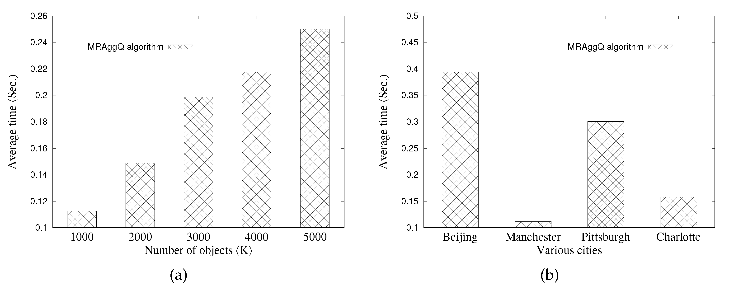
The second set of experiments illustrates the performance of processing the location-based aggregate queries using the Uniform dataset (in which the number of objects varies from 1000 K to 5000 K) and the real dataset (including the Beijing, Manchester, Pittsburgh, and Charlotte files). As shown in Figure 9a, the average running time for the MRAggQ algorithm increases with the increasing number of objects. The reason is that a larger number of objects results in more cells to be processed, so that a majority of the running time is spent on executing the Inner HNO set determining phase and the Outer HNO set determining phase. Nevertheless, benefited from processing the location-based aggregate queries in a distributed manner, the average running time for all cases remains below s. As for the real dataset, shown in Figure 9b, the Beijing file contains fewer objects than the Manchester, Pittsburgh, and Charlotte files, but incurs the highest average running time. This is because the Beijing file has a denser object distribution (compared to the other three files), thus leading to more HNO sets to be considered in the Aggregate-distance computing phase and the Result set generating phase.
5.4. Effect of Number of Object Types
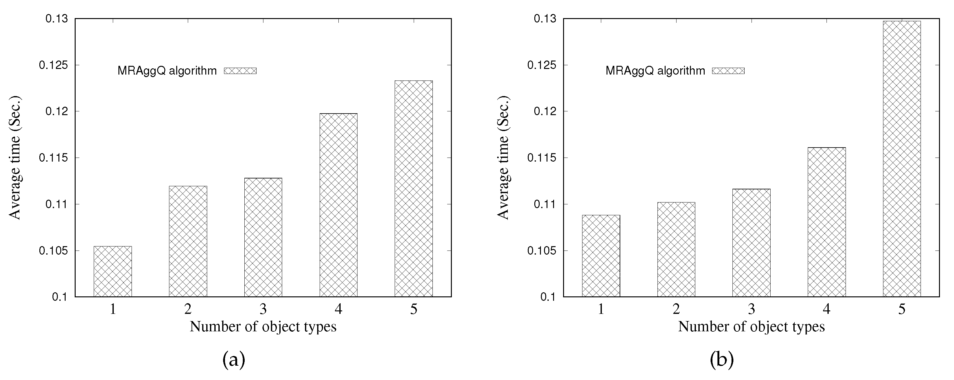
The third set of experiments is conducted to investigate the impact of the number of object types (i.e., the value of n) on the performance of the MRAggQ algorithm. Figure 10a,b measure the average running time of the MRAggQ algorithm for the Uniform dataset and the Manchester dataset, respectively, by varying n from 1 to 5. In the case where , implying that only single type of objects is considered, the processing cost required for determining whether the road distance between different types of objects exceeds the distance d can be completely avoided (that is, the first two phases of the MRAggQ algorithm do nothing). Moreover, the problem of processing the SAvgDQ, the SMinDQ, the SMaxDQ, and the SSumDQ is reduced to finding the nearest neighbor of the query object (i.e., the object with the shortest distance). In the case that n gets larger than 1, the Inner HNO set determining phase and the Outer HNO set determining phase need to be executed to find the HNO sets, as more than one type of object is processed. This is why the average running time of processing the location-based aggregate queries grows as the value of n increases. The experimental results also show that (1) the nearest neighbor query is a special case of location-based aggregate queries, where and , and (2) the proposed MRAggQ algorithm can be successfully applied to process the nearest neighbor query in a distributed manner.
5.5. Effect of Distance D
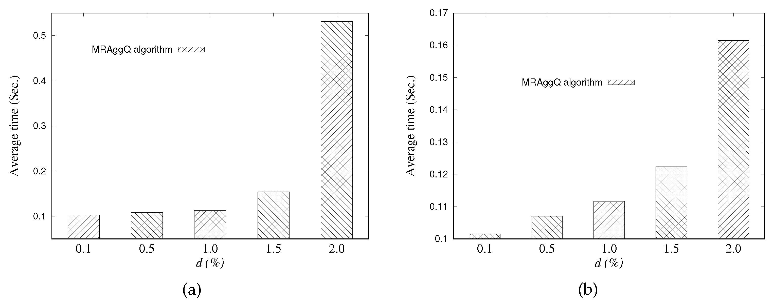
The fourth set of experiments illustrates the average running time of the MRAggQ algorithm as a function of the distance d (ranging from to of the width of the cell). As shown in Figure 11a,b, for both the Uniform dataset and the Manchester dataset, the larger the distance d, the higher the overhead in processing the location-based aggregate queries. This is attributed to the fact that, (1) for a smaller distance d, most of the object pairs cannot satisfy the constraint of distance d, reducing a lot of redundant distance computations in determining whether an object set can be the HNO set or not, and (2) a larger distance d makes the distance constraint easier to be satisfied for each object pair, incurring higher cost of computing object distances (in the Inner HNO set determining phase and the Outer HNO set determining phase) and more HNO sets to be considered (in the Aggregate-distance computing phase and the Result set generating phase).
5.6. Effect of Number of Query Points
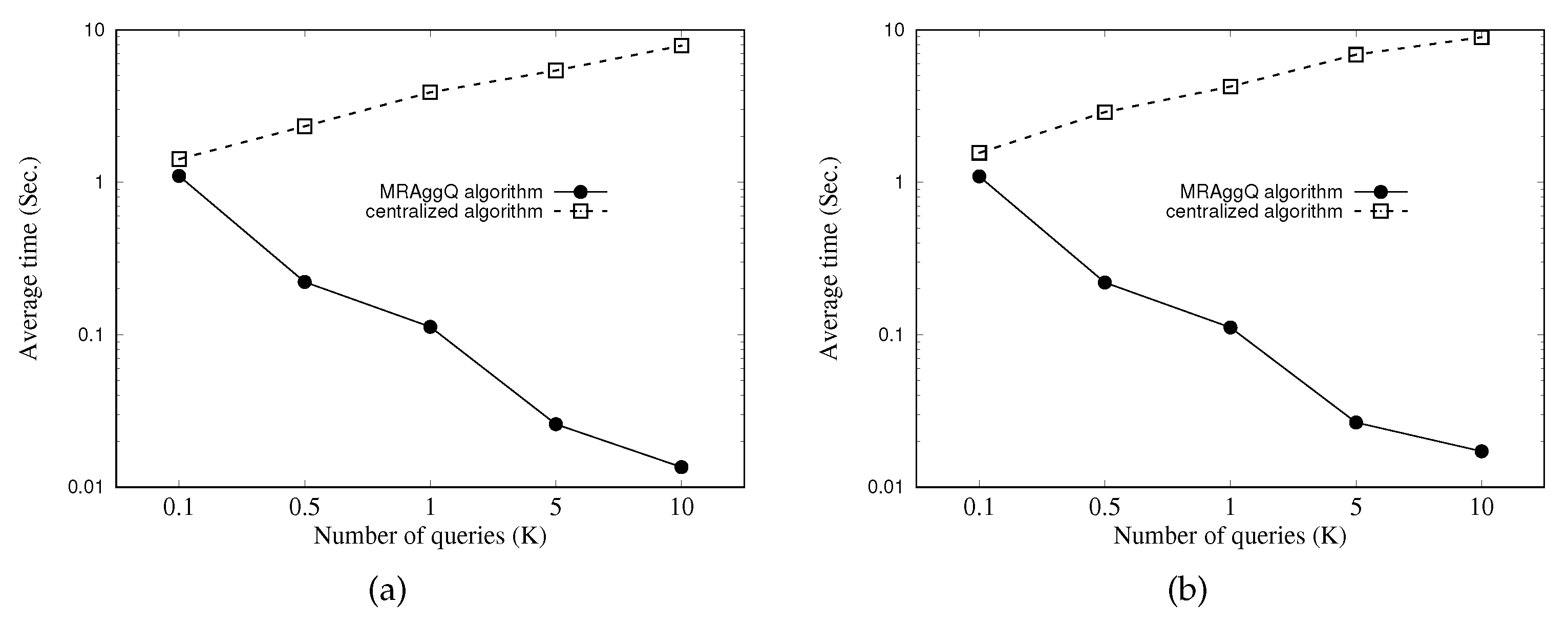
As the main focus of this paper is to process multiple location-based aggregate queries in a distribute manner, the scalability is the most important performance metric for the proposed MRAggQ algorithm—that is, the average CPU time it takes for the MRAggQ algorithm to simultaneously process multiple location-based aggregate queries. Therefore, in this subsection, a centralized approach proposed in the previous work [7], termed the centralized algorithm, is used as a competitor. The set of experiments demonstrates the scalability of the MRAggQ algorithm, compared to the centralized algorithm, by studying the effect of the number of location-based aggregate queries in terms of the average running time. Figure 12a,b evaluate the processing overhead for the Uniform dataset and the Manchester dataset, respectively, under various numbers of query points (varying from K to 10 K). Note that the two figures use a logarithmic scale for the y-axis. As we can see, both curves for the centralized algorithm exhibit the increasing trends with the increase of number of queries. This is because, in the centralized algorithm, the location-based aggregate queries need to be processed sequentially. It is very likely that the overall performance suffers from some time-consuming queries, and hence the average CPU time drastically increases for a large number of queries. Conversely, an interesting observation from the experimental results is that a larger number of queries results in a lower average running time for the MRAggQ algorithm. The reason for this improvement is that the increasing number of queries imposes only the computational burden on the last two phases (i.e., the Aggregate-distance computing phase and the Result set generating phase), instead of all the four phases of the MRAggQ algorithm. As a result, processing more queries would reduce more running time from the average perspective. The experimental results also show that there is a wide gap between the MRAggQ algorithm and the centralized algorithm, which confirms that the MRAggQ algorithm is scalable and efficient in highly dynamic environments where multiple location-based aggregate queries have to be processed concurrently.
6. Conclusions
In this paper, we focus on efficiently processing multiple location-based aggregate queries (including the SAvgDQ, the SMinDQ, the SMaxDQ, and the SSumDQ) in a distributed manner. We adopt the most notable MapReduce platform for parallelizing location-based aggregate query processing. A grid structure is first utilized to manage the heterogeneous objects by taking into account the storage balance, and then the MRAggQ algorithm is developed based on MapReduce, in which four MapReduce jobs are executed, to provide distributed processing of multiple location-based aggregate queries.
There are several interesting avenues for the future extensions of this work. One important research direction is to further improve the overall performance of the MRAggQ algorithm. For a heavy query load, the different keys may not be processed by different computing machines in parallel, thus decreasing the query performance. Therefore, our next step is to enhance the query performance by considering different clusters and/or Hadoop configurations (e.g., applying the SpatialHadoop). Then, an important avenue is to extend the distributed processing technique to be suitable for the environment where the heterogeneous objects move with time. Moreover, an extension is to address the issue of modifying the distributed processing technique to answer the location-based aggregate queries in road networks. Finally, a further extension is how to answer other variations of the location-based aggregate queries using a MapReduce platform.
Funding
This work was supported by the Ministry of Science and Technology of Taiwan under Grant MOST 107-2119-M-992-304 and Grant MOST 108-2621-M-992-002.
Conflicts of Interest
The author declares no conflict of interest.
References
- Benetis, R.; Jensen, C.S.; Karciauskas, G.; Saltenis, S. Nearest Neighbor and Reverse Nearest Neighbor Queries for Moving Objects. VLDB J. 2006, 15, 229–249. [Google Scholar] [CrossRef]
- Chen, J.; Cheng, R. Efficient Evaluation of Imprecise Location-Dependent Queries; ICDE: Oslo, Norway, 2007; pp. 586–595. [Google Scholar]
- Mokbel, M.F.; Xiong, X.; Aref, W.G. SINA: Scalable Incremental Processing of Continuous Queries in Spatio-temporal Databases. In Proceedings of the 2004 ACM SIGMOD, Paris, France, 13–18 June 2004; pp. 623–634. [Google Scholar]
- Sharifzadeh, M.; Shahabi, C. The Spatial Skyline Queries. In Proceedings of the International Conference on Very Large Data Bases, Seoul, Korea, 12–15 September 2006; pp. 751–762. [Google Scholar]
- Sistla, A.P.; Wolfson, O.; Chamberlain, S.; Dao, S. Modeling and Querying Moving Objects; ICDE: Oslo, Norway, 1997; pp. 422–432. [Google Scholar]
- Tao, Y.; Papadias, D. Time-parameterized queries in spatio-temporal databases. In Proceedings of the 2002 ACM SIGMOD, Madison, WI, USA, 3–6 June 2002; pp. 334–345. [Google Scholar]
- Huang, Y.K. Location-Based Aggregate Queries for Heterogeneous Neighboring Objects. IEEE Access 2017, 5, 4887–4899. [Google Scholar] [CrossRef]
- Dean, J.; Ghemawat, S. MapReduce: Simplified data processing on large clusters. In Proceedings of the 6th Symposium on Operating System Design and Implementation (OSDI 2004), San Francisco, CA, USA, 6–8 December 2004; pp. 137–150. [Google Scholar]
- Guttman, A. R-Trees: A Dynamic Index Structure for Spatial Searching. In Proceedings of the 1984 ACM SIGMOD, Boston, MA, USA, 18–21 June 1984; pp. 47–57. [Google Scholar]
- Papadopoulos, A.; Manolopoulos, Y. Multiple Range Query Optimization in Spatial Databases. In Proceedings of the ADBIS ’98, Poznan, Poland, 7–10 September 1998; pp. 71–82. [Google Scholar]
- Huang, Y.K.; Lin, L.F. Continuous Within Query in Road Networks. In Proceedings of the IWCMC 2011, Istanbul, Turkey, 5–8 July 2011; pp. 1176–1181. [Google Scholar]
- Iwerks, G.; Samet, H.; Smith, K. Continuous K-Nearest Neighbor Queries for Continuously Moving Points with Updates. In Proceedings of the International Conference on Very Large Data Bases, Berlin, Germany, 9–12 September 2003; pp. 512–523. [Google Scholar]
- Kalashnikov, D.V.; Prabhakar, S.; Hambrusch, S.; Aref, W. Efficient Evaluation of Continuous Range Queries on Moving Objects. In Proceedings of the International Conference on Database and Expert Systems Applications, Linz, Austria, 26–29 August 2002; pp. 731–740. [Google Scholar]
- Chung, B.S.; Lee, W.C.; Chen, A.L. Processing Probabilistic Spatio-Temporal Range Queries over Moving Objects with Uncertainty. In Proceedings of the EDBT 2009, Saint-Petersburg, Russia, 23–26 March 2009; pp. 60–71. [Google Scholar]
- Hjaltason, G.R.; Samet, H. Distance browsing in spatial databases. ACM Trans. Database Syst. 1999, 24, 265–318. [Google Scholar] [CrossRef]
- Roussopoulos, N.; Kelley, S.; Vincent, F. Nearest neighbor queries. In Proceedings of the 1995 ACM SIGMOD, San Jose, CA, USA, 22–25 May 1995; pp. 71–79. [Google Scholar]
- Chen, Y.; Patel, J.M. Efficient Evaluation of All-Nearest-Neighbor Queries; ICDE: Oslo, Norway, 2007; pp. 1056–1065. [Google Scholar]
- Xia, C.; Lu, H.; Ooi, B.C.; Hu, J. GORDER: An Efficient Method for KNN Join Processing. In Proceedings of the VLDB 2004, Toronto, ON, Canada, 31 August–3 September 2004. [Google Scholar]
- Papadias, D.; Shen, Q.; Tao, Y.; Mouratidis, K. Group Nearest Neighbor Queries; ICDE: Oslo, Norway, 2004; pp. 301–312. [Google Scholar]
- Bentley, J.L.; Kung, H.T.; Schkolnick, M.; Thompson, C.D. On the average number of maxima in a set of vectors and applications. J. ACM 1978, 25, 536–543. [Google Scholar] [CrossRef]
- Kung, H.T.; Luccio, F.; Preparata, F.P. On finding the maxima of a set of vectors. J. ACM 1975, 22, 469–476. [Google Scholar] [CrossRef]
- Borzsonyi, S.; Kossmann, D.; Stocker, K. The skyline operator. In Proceedings of the 17th International Conference on Data Engineering, Heidelberg, Germany, 2–6 April 2001; pp. 421–430. [Google Scholar]
- Hjaltason, G.R.; Samet, H. Incremental Distance Join Algorithms for Spatial Databases. In Proceedings of the International Conference on ACM SIGMOD, Seattle, WA, USA, 2–4 June 1998; pp. 237–248. [Google Scholar]
- Brinkhoff, T.; Kriegel, H.P.; Seeger, B. Efficient Processing of Spatial Joins Using R-trees. In Proceedings of the International Conference on ACM SIGMOD, Washington, DC, USA, 26–28 May 1993; pp. 237–246. [Google Scholar]
- Mamoulis, N.; Papadias, D. Multiway Spatial Joins. ACM Trans. Database Syst. 2001, 26, 424–475. [Google Scholar] [CrossRef]
- Zhang, D.; Chan, C.Y.; Tan, K.L. Nearest Group Queries. In Proceedings of the International Conference on SSDBM, Baltimore, MD, USA, 29–31 July 2013. [Google Scholar]
- Cary, A.; Sun, Z.; Hristidis, V.; Rishe, N. Experiences on processing spatial data with mapreduce. In Proceedings of the International Conference on Scientific and Statistical Database Management, New Orleans, LA, USA, 2–4 June 2009; pp. 302–319. [Google Scholar]
- Zhang, S.; Han, J.; Liu, Z.; Wang, K.; Feng, S. Spatial queries evaluation with mapreduce. In Proceedings of the International Conference on Grid and Cooperative Computing, Lanzhou, China, 27–29 August 2009; pp. 287–292. [Google Scholar]
- Ji, C.; Dong, T.; Li, Y.; Shen, Y.; Li, K.; Qiu, W.; Qiu, W.; Guo, M. Inverted grid-based knn query processing with mapreduce. In Proceedings of the ChinaGrid Annual Conference, Beijing, China, 20–23 September 2012; pp. 25–32. [Google Scholar]
- Ji, C.; Hu, H.; Xu, Y.; Li, Y.; Qu, W. Efficient multi-dimensional spatial RKNN query processing with mapreduce. In Proceedings of the ChinaGrid Annual Conference, Jilin, China, 22–23 August 2013; pp. 63–68. [Google Scholar]
- Akdogan, A.; Demiryurek, U.; Banaei-Kashani, F.; Shahabi, C. Voronoi-based geospatial query processing with mapreduce. In Proceedings of the International Conference on Cloud Computing Technology and Science, Indianapolis, IN, USA, 30 November–3 December 2010; pp. 9–16. [Google Scholar]
- Yokoyama, T.; Ishikawa, Y.; Suzuki, Y. Processing all k-nearest neighbor queries in hadoop. In Proceedings of the International Conference on Web-Age Information Management, Harbin, China, 18–20 August 2012; pp. 346–351. [Google Scholar]
- Zhang, C.; Li, F.; Jestes, J. Efficient Parallel kNN Joins for Large Data in MapReduce. In Proceedings of the EDBT 2012, Berlin, Germany, 27–30 March 2012. [Google Scholar]
- Lu, W.; Shen, Y.; Chen, S.; Ooi, B.C. Efficient processing of k nearest neighbor joins using mapreduce. In Proceedings of the International Conference on Very Large Data Bases, Istanbul, Turkey, 27–31 August 2012; pp. 1016–1027. [Google Scholar]
- Eldawy, A.; Alarabi, L.; Mokbel, M.F. Spatial Partitioning Techniques in SpatialHadoop. In Proceedings of the 41st International Conference onVery Large Data Bases, Kohala Coast, HI, USA, 31 August–4 September 2015. [Google Scholar]
- Eldawy, A.; Mokbel, M.F. SpatialHadoop: A MapReduce Framework for Spatial Data. In Proceedings of the 2015 IEEE 31st International Conference on Data Engineering, Seoul, Korea, 13–17 April 2015. [Google Scholar]
- Belussi, A.; Migliorini, S.; Eldawy, A. Detecting Skewness of Big Spatial Data in SpatialHadoop. In Proceedings of the 26th ACM SIGSPATIAL, Seattle, WA, USA, 6–9 November 2018. [Google Scholar]
- OpenStreetMap. Available online: http://www.openstreetmap.org/ (accessed on 23 August 2019).
Figure 1.
Example of processing the location-based aggregate queries. (a) Heterogeneous objects; (b) Multiple queries.
Figure 1.
Example of processing the location-based aggregate queries. (a) Heterogeneous objects; (b) Multiple queries.

Figure 2.
Illustration of grid structure and HDFS. (a) Heterogeneous objects; (b) Grid structure; (c) Data on HDFS.
Figure 2.
Illustration of grid structure and HDFS. (a) Heterogeneous objects; (b) Grid structure; (c) Data on HDFS.

Figure 3.
Flowchart of the MRAggQ algorithm.

Figure 4.
Illustration of the Inner HNO set determining phase.

Figure 5.
Illustration of the Outer HNO set determining phase.

Figure 6.
Illustration of the Aggregate-distance computing phase.

Figure 7.
Illustration of the Result set generating phase.

Figure 8.
Effect of the parameter . (a) Uniform dataset; (b) Manchester dataset.

Figure 9.
Effect of the number of objects. (a) Uniform dataset; (b) Real dataset.

Figure 10.
Effect of the number of object types. (a) Uniform dataset; (b) Manchester dataset.

Figure 11.
Effect of the distance d. (a) Uniform dataset; (b) Manchester dataset.

Figure 12.
Effect of the number of queries. (a) Uniform dataset; (b) Manchester dataset.


Table 1.
System parameters.
| Parameter | Default | Range |
|---|---|---|
| Parameter | 1000 | 250, 500, 1000, 1500, 2000 |
| Number of objects (K) | 1000 | 1000, 2000, 3000, 4000, 5000 |
| Number of object types | 3 | 1, 2, 3, 4, 5 |
| Distance d (%) | 1 | , , 1, , 2 |
| Number of query points (K) | 1 | 0.1, 0.5, 1, 5, 10 |
© 2019 by the author. Licensee MDPI, Basel, Switzerland. This article is an open access article distributed under the terms and conditions of the Creative Commons Attribution (CC BY) license (http://creativecommons.org/licenses/by/4.0/).
Share and Cite
MDPI and ACS Style
Huang, Y.-K. Distributed Processing of Location-Based Aggregate Queries Using MapReduce. ISPRS Int. J. Geo-Inf. 2019, 8, 370. https://0-doi-org.brum.beds.ac.uk/10.3390/ijgi8090370
AMA Style
Huang Y-K. Distributed Processing of Location-Based Aggregate Queries Using MapReduce. ISPRS International Journal of Geo-Information. 2019; 8(9):370. https://0-doi-org.brum.beds.ac.uk/10.3390/ijgi8090370
Chicago/Turabian StyleHuang, Yuan-Ko. 2019. "Distributed Processing of Location-Based Aggregate Queries Using MapReduce" ISPRS International Journal of Geo-Information 8, no. 9: 370. https://0-doi-org.brum.beds.ac.uk/10.3390/ijgi8090370
Note that from the first issue of 2016, this journal uses article numbers instead of page numbers. See further details here.