Article

A Filtering-Based Approach for Improving Crowdsourced GNSS Traces in a Data Update Context

by
Stefan S. Ivanovic
1,*,
Ana-Maria Olteanu-Raimond
1,
Sébastien Mustière
1 and
Thomas Devogele
2
1
Univ. Paris-Est, LASTIG, MEIG, IGN, ENSG, F-94160 Saint-Mandé, France
2
Université de Tours, Laboratoire D'informatique LIFAT, 41000 Tours, France
*
Author to whom correspondence should be addressed.
ISPRS Int. J. Geo-Inf. 2019, 8(9), 380; https://0-doi-org.brum.beds.ac.uk/10.3390/ijgi8090380
Submission received: 4 July 2019 / Revised: 14 August 2019 / Accepted: 21 August 2019 / Published: 30 August 2019

Abstract

:
Traces collected by citizens using GNSS (Global Navigation Satellite System) devices during sports activities such as running, hiking or biking are now widely available through different sport-oriented collaborative websites. The traces are collected by citizens for their own purposes and frequently shared with the sports community on the internet. Our research assumption is that crowdsourced GNSS traces may be a valuable source of information to detect updates in authoritative datasets. Despite their availability, the traces present some issues such as poor metadata, attribute incompleteness and heterogeneous positional accuracy. Moreover, certain parts of the traces (GNSS points composing the traces) are results of the displacements made out of the existing paths. In our context (i.e., update authoritative data) these off path GNSS points are considered as noise and should be filtered. Two types of noise are examined in this research: Points representing secondary activities (e.g., having a lunch break) and points representing errors during the acquisition. The first ones we named secondary human behaviour (SHB), whereas we named the second ones outliers. The goal of this paper is to improve the smoothness of traces by detecting and filtering both SHB and outliers. Two methods are proposed. The first one allows for the detection secondary human behaviour by analysing only traces geometry. The second one is a rule-based machine learning method that detects outliers by taking into account the intrinsic characteristics of points composing the traces, as well as the environmental conditions during traces acquisition. The proposed approaches are tested on crowdsourced GNSS traces collected in mountain areas during sports activities.

1. Introduction

With the development of Web 2.0 techniques for sharing information or the increasing ease of positioning thanks to the Global Navigation Satellite System (GNSS), citizens can act as sensors and produce geographic data, which is emphasized by the word ‘producer’ proposed by [1]. In geographic information science (GIS), various concepts are being used to define that trend [2], such as neogeography [3], volunteered geographic information (VGI) [4], user generated spatial content [5], or crowdsourcing and community sourcing [6].
In particular, the increasing amount of crowdsourced GNSS traces shared by citizens in the context of their sports and spare time activities, like hiking or biking, provides rich information about the use of roads and paths. These traces may be explored in various contexts such as behaviour analysis, the estimation of human pressure on protected natural areas, or the improvement of displacement facilities [7,8,9]. The research work presented in this paper focuses on the use of crowdsourced traces aiming to improve the actuality of authoritative data. Our research assumption is that crowdsourced traces may be used by data producers, such as national mapping agencies (NMAs), to detect potential changes on the ground, in particular when changes occur quickly and detection by image analysis is costly or even not possible (e.g., in forest area where footpaths cannot be seen on images or in cloudy areas where it is difficult to capture aerial or satellite images). Crowdsourced traces may highlight missing footpaths in authoritative datasets or confirm that some footpaths are still in use.
However, crowdsourced traces have limitations. First, data made available through website or social networks are usually poorly described: Citizens share only the main information (latitude, longitude, altitude and timestamp of each point) but do not save and share metadata that could help to determine their quality (e.g., number of visible satellites when collecting the data or type of GNSS device used). Second, even if the quality has been increasing continuously through the years, this data still contain too many outliers and sometimes insufficient positional accuracy for some purposes [10]. In some contexts, such as updating major road networks from GNSS traces collected by devices imbedded in cars, the limited quality of GNSS data may be counteracted by the huge amount of available traces. In the footpath context, it may be expected that data are rich enough for detecting potential updates. However, few GNSS traces follow the same path, with poor metadata, attribute incompleteness and heterogeneous accuracies. In some cases, there are no protocols for collecting crowdsourced data, whereas in some other cases, protocols exist but they are not always detailed or respected by contributors [11]. The lack of protocols implies a spatial, thematic and semantic heterogeneity of collected crowdsourced data. Moreover, the significant variety of sensors and methods applied for data acquisition results in a random distribution of quality. Crowdsourced data present four main characteristics rising issues in our context: High spatial and temporal heterogeneity, incompleteness, lack of metadata, and lack of redundancy.
In this research work, a crowdsourced trace is composed of a set of trace points that have geographic coordinates, timestamps and elevation. The points are captured during the movement of a person from an origin A to a destination B. Each point represents the location of a contributor at a given time (see Figure 1a).
On the one hand, during the movement, different activities may be made such as walking by following an existent path or going off an existing path (off-road movements) for different reasons (e.g., having a break in the nearby meadow or visiting an area of interest). Two types of behaviour are identified: Main behaviour (i.e., the contributor sticks to the previously planned itinerary) and secondary behaviour (i.e., the contributor makes activities out of the main path such as taking a break, taking pictures, or seeing a view). The latter is named in this paper secondary human behaviour (SHB) and is considered as local geometric noise of a trace containing irrelevant information for purposes focused on displacement.
On the other hand, many factors may influence the accuracy of a point during the acquisition process generating errors with respect to the real position of the contributor. These errors are named in the following “outliers”.
The goal of this paper is to detect and filter both secondary human behaviour and outliers in order to improve the smoothness of the crowdsourced traces. The result is a smooth trace that has geometric characteristics closer to topographic paths, as illustrated in Figure 1b.
The main question of this paper is: Is it feasible to filter GNSS traces to obtain traces that have enough accuracy to detect updates in authoritative data? Knowing the two types of noise to filter, the secondary questions are: How can one detect secondary human behaviour in traces that have an aleatory presence of timestamps and poor semantic information? Which are the indicators and thresholds to take into account to detect outliers in heterogeneous traces? Finally, is it feasible to define a generic method based on these indicators?
This paper is organized as follows. First, the relevant literature on detecting stops and outliers as well as on factors influencing GNSS measurements is presented in Section 2. The proposed approach for filtering crowdsourced traces is described in Section 3. Before concluding in Section 5, experimental results are presented in Section 4.

2. Literature Review
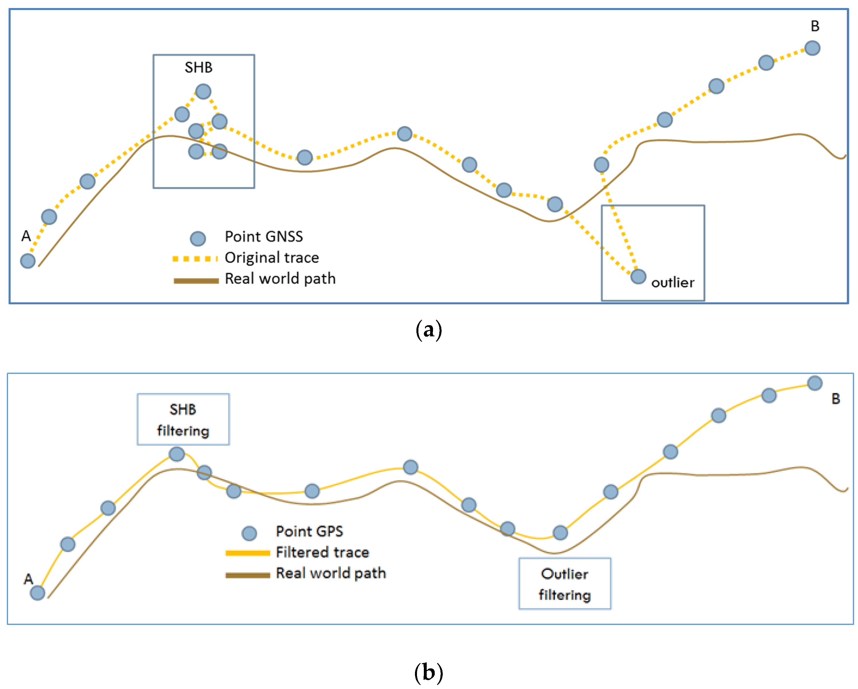
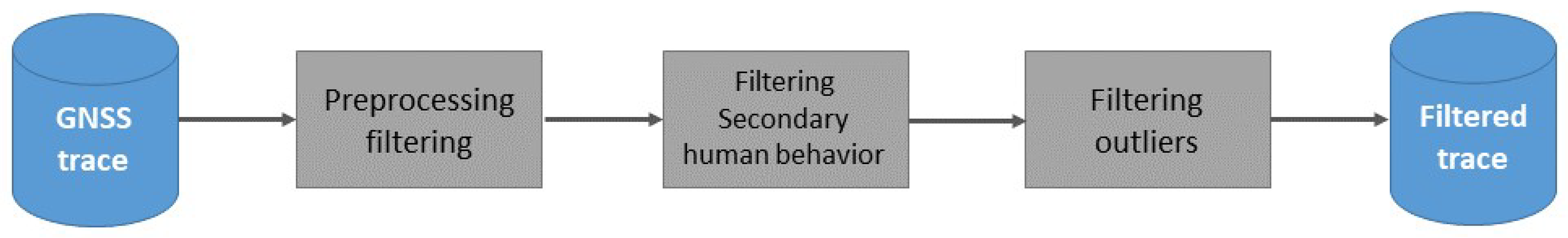
As previously mentioned, crowdsources traces come from human sports activities following existing roads or footpaths and according to planned itineraries.
Detecting SHB and hiding it is useful in the context of authoritative data update. This phenomenon is broadly known as stops in human mobility [12]. Most of the methods for detecting stops rely on spatial information [13,14], spatiotemporal information [15,16,17,18] and temporal information [19,20]. However, those methods cannot be applied to detect SHB when a considerable amount of points are affected by missing timestamps or when the high spatiotemporal resolution heterogeneity makes difficult to determine threshold settings.
To detect outliers, we focused our review of the literature on two topics. The first concerned the methods proposed in the literature to detect outliers in traces. The second concerned the factors that may be considered as sources of errors in GNSS measurements.
GNSS traces are sometimes significantly degraded by the presence of outliers. Several outlier detection approaches may be distinguished: Some based on detecting GNSS measurement errors that lead to outliers and others based on detecting outstanding geometries anomalies among several traces. In the first group, the assumption is that outlying observation conditions produce geometric incorrectness and anomalies in GNSS data. Considering this assumption, some approaches consider measurements of pseudo-ranges as the most successful indicator for detecting outliers in GNSS measurements [21,22]. Other approaches consider speed and timestamp for detecting outliers provoked by the effects of GNSS data logging errors, i.e., sudden signal loss, data spiking, signal white noise, and zero speed drift [23,24,25] applied a Kalman filter for refining traces geometry especially on the outlier points. In the second group of approaches, an outlier is a point, segment or trace, which differs from the mean shape of other traces following the same path [26,27]. Outliers may be found by means of 3D axis calculated based on intersections of traces and perpendicular planes along the path [26]. A point is then considered an outlier if the distance to the mean axis is greater than a threshold.
The former approach needs complete and reliable raw measurements, whereas the latter requires a sufficient number of traces following the same itinerary. Regarding the footpath update study we are conducting, none of these conditions were fulfilled. First, publicly available crowdsourced data do not often contain raw GNSS measurements and have missing metadata. Second, in some harsh areas such as mountains, there is a lack of crowdsourced traces and the number of traces following the same itinerary is low (from one-to-three in our test area). A Kalman filter is also difficult to adapt in the mountain context, since the effect of its application can be the exaggerated smoothing of winding roads.
The quality of trace depends on the quality of the GNSS device being used and the spatial context. Hence, our idea was to define a set of intrinsic and extrinsic indicators to possibly characterize errors in GNSS data. Defining indicators based on different characteristics is also a common approach when dealing with crowdsourced data quality assessment [28]. For example, [29] proposed a set of intrinsic (i.e., based on analysing solely characteristics of crowdsourced data) and extrinsic (i.e., based on comparing crowdsourced data to authoritative data) indicators. The intrinsic indicators are ad-hoc defined. They describe local knowledge defined as familiarity of the user to an area [30], reliability [31,32], and expertise [33]. Extrinsic indicators are based on the quality elements proposed by International Organization for Standardization ISO 19157 [34,35,36,37] or other types of data characterizing the spatial context of traces [28,32,37,38]
The sources of errors of GNSS receivers, such as ionospheric and tropospheric effects, errors of receiver clocks, number and spatial distribution of visible satellites, or reflections of the signal, are well known [39]. In practice, those errors arise in different configurations. Studies performed in the scientific literature were carried out under various conditions, still comparing an impact of each factor is not straightforward. In the framework of outdoor sports activities, the most influencing configurations affecting the quality of traces seem to be the following: Canopy cover, type of GNSS device, position of receiver, topography, and measurement duration.
Canopy cover and its density are recognized as the most influencing factors on GNSS collection process [40,41,42]. The number of satellites and the signal quality varies depending on the characteristics of the canopy cover, which has a direct impact on the position accuracy [42] or the length of collected traces [41].
Different types of GNSS devices exist based on electronic components with different qualities or based on different technics. Among those technics, a significant difference exists between differential and non-differential GNSS (i.e., without position corrections from base station), with the former producing a greater positional accuracy as well as a greater number of acquired positions, particularly in challenging environmental conditions [40].
The position of receiver while collecting data also has a significant effect. Studies show that the orientation of a device consistently influences both the fix rate (from 100% to 80%) and positional accuracy (from a few meters to twenty meters) according to some experiments performed under dense canopy cover. However, this tends to have a negligible effect on GNSS errors in open areas. [43,44,45,46] similarly showed that positional accuracy is impacted by how a GNSS receiver was carried while collecting data (e.g., in a pocket or in a hand).
The conclusions of studies evaluating the influences of topography (e.g., local slope) are divided. Some showed no statistically significant differences between the positional error of points acquired in locations with different topographic characteristics [47,48], whereas others detected a relation between positional accuracy and topographic conditions [41,42,49]. Finally, some studies showed negative effects of topography on the success of acquiring 3D positions [42,49].
Additionally, some studies showed that the fix success rate decreases gradually as measurement duration rose (e.g., from 99.6% for 15 min of measurement time to 92% for 13 h) [40,49]. To go further, such studies should be extended because they do not sufficiently prove the influence of measurement duration in different configurations.

3. Methodology

This section describes the approach proposed for filtering both secondary human behaviour and outliers in crowdsourced traces in order to obtain a smooth trace that is more suitable for usages such as updating authoritative data. The variety of sources of errors on the one hand and the fact that publicly available data are poorly described and very heterogeneous on the other hand led us to propose a general approach which relies only on the shape and temporal aspects of traces without any prior knowledge about data capture conditions.
The proposed methodology consists of three main steps, as illustrated in Figure 2. The first step is the pre-processing filtering. The second step consists of detecting the points representing secondary human behaviour. Finally, the outliers are detected and eliminated by applying a rule-based filtering. The result of the methodology is a filtered trace with more accurate geometry.

3.1. Pre-Processing Filtering

As described in [50], each trace has to undergo preliminary filtering, including deleting redundant points (i.e., consecutive points at the same position) and negative speed values, as well as correcting values for timestamp and elevation. In some traces—Besides regular and NULL elevation and timestamp values—One may get a zero value or an identical value for all points, certainly due to GNSS receiver errors or data format issues when downloading or uploading traces. To avoid introducing errors, every timestamp and elevation value is replaced with a NULL value in these cases.

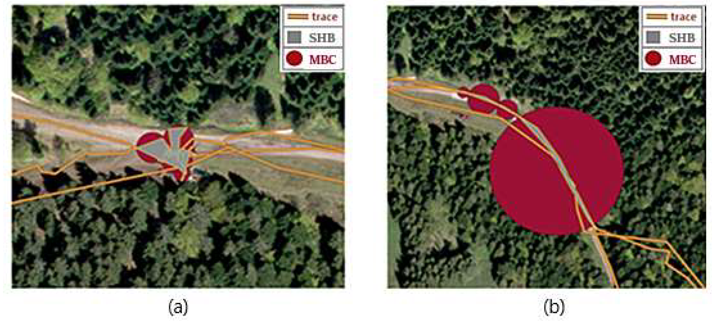
3.2. Filtering Secondary Human Behaviour

Secondary human behaviour bears two characteristics: A relevant change of direction between segments and trace self-intersection. To identify SHB, polygons defined by the parts of the trace that self-intersect are built (see Figure 3a). Then, both area and elongation are computed for each polygon. Finally, polygons that have area and elongation less than thresholds TA (threshold area) and TE (threshold elongation) respectively are identified as SHB, and all the points composing these polygons are considered to be results of SHB. To avoid new self-interactions after having filtered points identified as SHBs, the process is carried out iteratively until eliminating all self-intersections.
The elongation is defined for each polygon as the ratio between the area of the polygon and the area of the minimum bounding circle (MBC) of the polygon.
Figure 3 illustrates the computed polygons of a real SHB and a round-trip trace. The elongation criterion allows us to differentiate real SHBs (Figure 3a) from other configurations (e.g., round trips), as illustrated in Figure 3b.
Note that, in our approach, the points identified as results of an SHB are filtered and the trace is rebuilt.

3.3. Filtering Outliers

As proposed in [50], an outlier can be defined as a point whose metric and geometric characteristics differ significantly from the characteristics of other points composing its full trace. The method consists of first defining intrinsic and extrinsic indicators describing each point of a trace; second, examples of outliers and not-outliers are manually labelled; finally, a rule-based learning algorithm is applied. The choice is motivated by the fact that a rule-based learning algorithm allows for interactive modifications or improvements of learnt rules, which is not possible with non-symbolic classification algorithms. The indicators are defined and discussed in the next section.

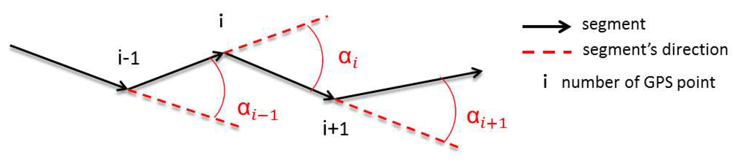
Definition of Intrinsic and Extrinsic Indicators for Describing GNSS Points

The intrinsic indicators are calculated by using traces themselves, whereas the extrinsic indicators are derived from an analysis of the spatial context in which trace points are collected, such as the type and density of forest, the slope or the proximity of obstacles (e.g., cliffs and buildings). Globally, 15 indicators are defined: eight of them are intrinsic (see Table 1), whereas seven are extrinsic.
AngleMean measures the change of direction of a trace over consecutive segments (see Figure 4). It is an important characteristic of outliers, since most of them make a significant direction change in a trace. Inasmuch as the geometry of a regular trace can have significant direction changes (e.g., when turning), our indicator considers changes of direction for the preceding and succeeding points in the trace.
DistDiffN and SpeedDiffN register sudden changes in speed and distance between consecutive points. Di and Vi represent, respectively, the distance and the speed between points i, and i − 1. Similarly, SpeedRate represents the velocity change rate as suggested by [51].
SpeedMean and DistMean represent the average speed and distance values to preceding and following points, respectively.
DistDiffMed is the ratio between the local segment lengths (average of lengths of preceding and succeeding segments) and the median length of every segment of the trace. In this way, the spatial resolution of a given trace is taken into account, and its discrepancies are modelled.
DiffEle is the maximum difference in elevation from one point to the preceding and following points, as determined by elevation (Z) values in GNSS data.
The extrinsic indicators are listed in Table 2 and described in the following. They model factors influencing GNSS measurements as described in Section 2. To compute the extrinsic indicators, three types of authoritative data coming from the topographic database (named BDTopo), produced by the French National Mapping Agency (IGN), and with metric accuracy and are used: Digital Terrain Model (DTM) raster data and building and land cover vector data.
DiffEleDTM is an extrinsic indicator and assesses the accuracy of GNSS elevation on one point. This indicator is based on the idea that significant errors in elevation are usually related to significant errors in 2D position [52]. It requires using a precise DTM of the area to be measured: The elevation of GNSS data is compared to the elevation at the same x, y position on the DTM.
Slope is the gradient of altitude at the location derived from the underlying referential DTM.
The Obstacles indicator provides an estimate of the multipath effect, one of the most influential factors in GNSS accuracy. It considers the proximity of obstacles (e.g., within 10 m) that contribute to multipath within our test environment, namely buildings and forests. Building- and land-cover maps from an authoritative dataset are used to compute this indicator. The threshold for defining close features is related to the average precision expected from a smartphone GNSS and the precision of the reference data. This could be refined with distance thresholds related to the height of obstacles.
Curvature represents the convexity of slope.
Vegetation represents the land cover class at the position of the point, as defined by a reference land cover map (LCM).
CanopyCover states whether the point is in the forest or not, according to a reference LCM.
InBuildingWater is an indicator that identifies inconsistencies. Due to the imprecision of GNSS, some points can be located in water or on building surfaces according to an authoritative dataset. This reflects an inconsistency with normal hiking/cycling activities and is therefore a clue for an outlier.
A majority of these indicators were defined by the authors of this paper to appropriately model the most important metric and geometric characteristics of the outliers. Some other indicators such as speed rate were used since they have already been successfully used in trace analytics.

4. Experimental Results

The proposed approach was applied to real data representing crowdsourced GNSS traces collected in mountain area. For visualization purposes, authoritative roads from BDTopo produced by the French Mapping Agency (noted as IGN in figures) were used.

4.1. Test Data Description

The test area was in the Vosges Mountains (France). It was chosen for its interesting characteristics: It is a small, mountain-mixing, dense forest with different canopies and open areas. For our study, a total of 437 traces (9773 km) were downloaded from hikers and mountain bikers’ websites (randoGPS, tracesGPS, visuGPS, and VTTour) sharing GNSS traces. The traces were collected while performing sports activities such as running, hiking and cycling. Since traces were collected without a data collection protocol and since no metadata were available, no distinction was made according to the transportation mode (e.g., walking, running, or biking), and no information was available about their expected spatiotemporal resolution.
The completeness and heterogeneity of this data are described below. Points were theoretically described by, at least, 2D coordinates (World Geodetic System 1984-WGS-84), timestamps, and elevation. Among 300,000 points, 106,206 points (36.3%) lack timestamps, and 6580 points (2.2%) lacked elevation. Regarding the traces, 157 of them (35.9%) had no timestamps at all, whereas 287 (65.6%) had at least one missing timestamp. Timestamps are important information necessary for different analyses (e.g., speed or acceleration). This random distribution of timestamps and a particularly huge number of traces with no timestamps at all (35.9%) were significant issues when trying to use this data and assessing their quality.
To evaluate the heterogeneity of crowdsourced traces, the distributions of data frequency, speed (if timestamped) and distance between consecutive points within each trace were studied. Statistical tests such as Shapiro—Wilk, skewness and kurtosis (K) tests showed that speed and distance are rarely normally distributed. For example, less than 7% of traces were normally distributed for speed, and no traces were normally distributed for distance. Moreover, it was noticed that different distributions of speed values between traces existed (see Figure 5).
Figure 6 illustrates the variation of skewness of speed values for all traces. The variety of speed distribution within each trace is illustrated by the variety of skewness estimation for all traces. This may be explained by frequent changes in the speed during a trip (e.g., by bike and on foot) required, for example, by rough relief in a mountainous area as well as different sampling rates. This is a critical point for detecting outliers in crowdsourced traces because simple thresholds on length or speed to determine outliers or low accuracy points are not sufficient.

4.2. Detection of Secondary Human Behaviour

The algorithm presented in Section 4.2 allowed us to detect 11,746 (4%) points as results of SHB. The algorithm was run until no points belonging to SHB remained (three iterations). The thresholds for areas and elongation criteria were empirically, respectively, set to 200 m2 and 0.13. The method was successful in various types of SHB. Both simple and very complex SHBs were eliminated. Typical results are shown in Figure 7.
A detailed and quantitative validation of the results was conducted on 14 randomly selected traces representing 265 km. Overall, 204 SHB points were detected by the method—three falsely—but 16 real SHB points remained undetected. Hence, both the precision (98%) and recall (93%) of the method are high.

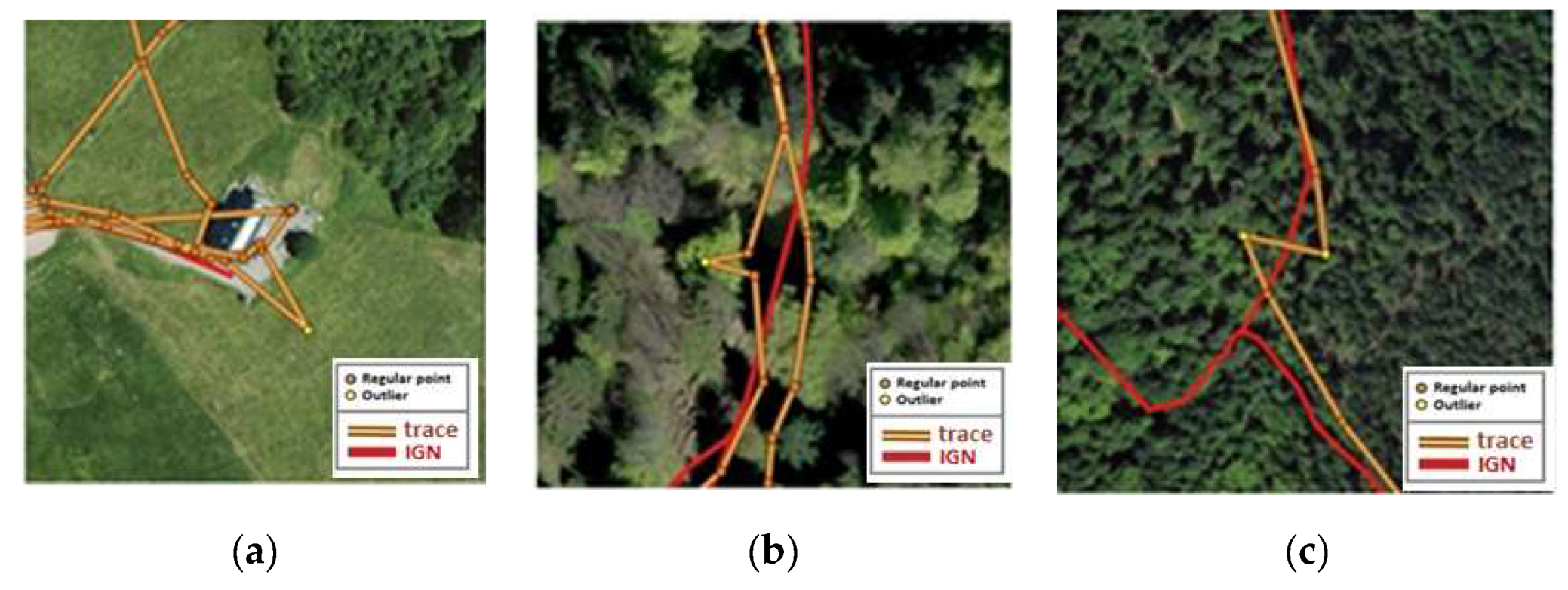
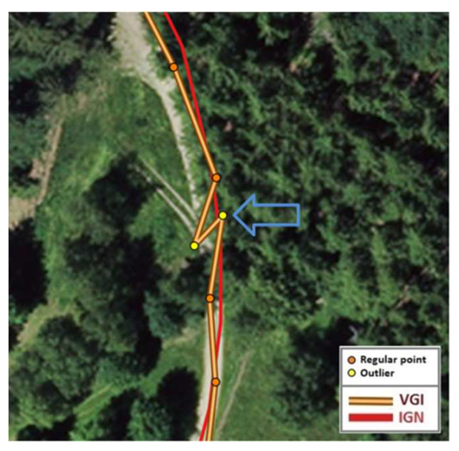
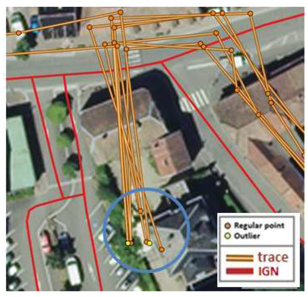
4.3. Detection of Outliers

The detection of outliers was carried out by following four steps: (i) Defining training examples, (ii) applying a machine learning algorithm, (iii) a quantitative validation, and (iv) a qualitative validation.
The first step consisted of defining training examples. Thus, a training area was selected, and each training example was manually labelled with two values: Outlier or regular point. In the sampling zone illustrated in Figure 8 (black boxes), 2342 points were selected and manually labelled as outliers or regular points. Among the total number of points, 35 (3%) points were labelled as outliers and 2265 (97%) were labelled as regular points. Clearly, the learning dataset was very imbalanced (one outlier within 66 regular points). To reduce the bias, 77 examples of outliers beyond the sampling zone were added to the training dataset. In this way, the statistical representativeness of the examples was lost, but more examples of outliers were obtained with limited effort.
The second step was the learning process. As stated before, a rule-based learning algorithm was chosen to enable interactive modifications or improvements of learnt rules, which is impossible with non-symbolic classification algorithms. In addition, they are known as efficient and able to deal with examples described by numeric, qualitative, and possibly missing attributes [53]. By using Weka software package, four different rule-based algorithms were applied: Repeated Incremental Pruning to Produce Error Reduction (RIPPER), Projective adaptive resonance theory (PART), M5Rules, and One attribute rule (OneR).
The third step was the quantitative validation. The validation of results was performed using 10-fold cross validation in order to ensure a statistically unbiased evaluation knowing the low number of examples. Validation results of the four applied algorithms are presented in the Table 3.
Overall, the RIPPER algorithm performed best. The validation results gave both precision and recall equal to 79%, and the F1 measurement equalled 0.79.
The results confirmed the performance of the approach and learnt rules, in spite of the lack of metadata as well as the presence of missing attributes. Finally, five following rules were learnt to detect outliers (see Table 4).
The learnt rules were applied individually on unclassified points from the test area (i.e., all the GNSS points not used for learning rules). As a result, 9303 points (3%) were detected as outliers.
Finally, the last step was the qualitative validation performed by visual interpretation of different Web Map Tile Services (orthophotos and maps) coming from the French geoportal (https://www.geoportail.gouv.fr/).
Rule 1 detected outliers with a sharp direction change, close to 90° and corresponding distances slightly greater than the mean value of spatial resolution of the entire trace (see Figure 9a). This rule could be applied to traces, whether they had timestamps or not. In total, 1461 points were detected by Rule 1.
Rule 2 detected outliers with notable speed and direction changes, as shown in Figure 9b. The application of Rule 2 resulted in 2076 points detected as outlying.
Rule 3 detected a sharp deformation in trace geometry—sharp in terms of direction—but not distant from the trace main axis (see Figure 9c). The rule was applicable to traces whether they had timestamps or not. Overall, 3622 outliers were detected by this rule.
Rule 4 detected 2135 outliers, those similar in a geometric sense to the outliers detected by the Rule 3, however Rule 4 was more successful with the traces not affected by missing timestamps. Finally, Rule 5 detected outlying points being very distant from the trace main axis; those cases were rare (only nine points) but had a strong adverse effect on the smoothness of the trace.
In the following, some false-positive and false-negative results are illustrated. The analysis of the false-positive outliers showed that they mainly resulted from side-effect caused by the AngleMean indicator. This is not surprising, since the outliers affect significantly intrinsic indicators of neighbouring points in a trace, especially direction changes measured by the AngleMean indicator. A typical example of false positive outlying point is labelled by the blue arrow in Figure 10.
As illustrated in Figure 11, traces with low spatial resolution and high sinuosity contained most of the false positive results in outlier detection. Points composing such traces were very similar to outliers regarding their metric characteristics. Such points were mainly falsely detected as outliers despite them having accurate positions. All five GNSS points (represented in yellow—figure on the left) were wrongly identified as outliers. However, we noticed that the results were different for high sinuosity paths and good spatial resolution of traces (see Figure 11). The method performed better for traces with good spatial resolution whatever the sinuosity of paths.
An analysis of false negative results showed they were mostly inducted by a sensibility of thresholds. Figure 12 shows outlying points not detected as outliers (orange points within the blue circle) due to a slight difference between the values of the indicator AngleMean and the learnt threshold. All differences for the orange points blue circle are less than 1°. This result confirms the difficulty to define thresholds for detecting outliers in crowdsourced traces.

5. Discussion and Conclusions

More and more contributors are using smartphone GNSS devices in their sports and leisure activities. The amount of crowdsourced data is increasing day by day, as is the number of possible usages. One of them is to use crowdsourced trace to update authoritative data. In this context, it is essential to filter the noise of traces in order to obtain smooth traces that have closer geometric properties to a topographic path. As far as we know, little research has dealt with crowdsourced GNSS traces in real conditions where there is little or no metadata at all, few redundant data (traces following the same path), and high heterogeneity within the data.
In this paper, we proposed an approach for improving the geometry of crowdsourced GNSS traces by filtering secondary human behaviour and outliers. The method proposed for detecting SHB is a geometric-based approach. The method for detecting outliers is based on machine learning techniques to determine relevant indicators and thresholds. Both methods were tested on real data in a mountainous area.
The SHB method proved to be efficient in in this study by filtering 10,315 points representing 3.6% of the total points. Good precision and recall were obtained (P = 98%, R = 93%). Furthermore, its limitations were offset by the fact it performed well even on poor data with missing timestamps, spatial heterogeneities, and no metadata. Moreover, the method was independent of transportation mode classification and missing attributes compared to most of existing stop detection methods.
In the context of updating authoritative data, SHB was considered noise. This is not necessarily the case for other purposes such as human mobility analysis or land cover changes detection. For these studies involving any mobile object such as humans, animals, cars, detecting places where an activity is carried out is very useful and currently studied in the literature. Our method could be used for those purposes, but more research would then be necessary to determine the shape of the stop and to assign semantic information such as the types of activities. This is a difficult task when a timestamp is missing, since the type of activity is closely linked to the duration of stops. If a better completeness of attributes (especially timestamps) was had, identifying the mode of transportation (e.g., walking or cycling) and comparing the accuracies of traces with respect to the transportation mode would be relevant research in the field of human mobility. Using the spatial context or matching traces with its textual description where available, as in [54], may also be explored.
The method proposed for detecting outliers defines intrinsic and extrinsic indicators and uses machine learning techniques to generate rules and thresholds. Five different rules combining five different indicators were learnt, filtering 3% of points detected as outliers. This confirms that detecting outliers in crowdsourced GNSS traces is a complex task that cannot be solved through a single threshold on only one indicator. One other important finding is that intrinsic indicators are sufficient for outlier detection. This may be surprising regarding the current understanding of the effect of external conditions, particularly canopy cover [42,55]. However, this may be explained by the lack of accuracy and poor resolution of the geographic data sources used (digital terrain model and land cover map). It may also be that external conditions alone, without information on GNSS receivers, are not sufficient. For example, the same obstacle may reflect the GNSS signal and subsequently produce an outlier when collecting data with low quality GNSS, whereas it is not the case with high precision GNSS under the same conditions. Among intrinsic criteria, the criteria based on change direction between consecutive points (i.e., AngleMean) proved to be the most relevant, which is not surprising since geometric anomalies of a trace have significant direction changes.
The main advantage of the proposed method is that it is not affected by: (1) The transportation mode of traces—generally the first step of the majority of outlier and stop detection methods in traces analysis; (2) data redundancies, since the traces are analysed one by one, and, as such, no redundancies in traces following the same path are needed; (3) missing attributes, since the methods can be applied on traces with missing attributes. Let us mention that if timestamps are available, they may be taken into account and improve results, but, if not, other rules may be used to detect some outliers.
Regarding the training data, ideally, the sampling zone should be as wide as possible and should represent the state and heterogeneities of the entire test area and the entire pattern of points as much as possible. In practice, because this task is relatively time-consuming and the number of non-outlier points is largely greater than the number of outlier points, there may be an issue. In fact, determining a sufficient number of outlier examples would require examining a very large amount of points, which is difficult in practice. Moreover, our data were imbalanced, which was reported as an issue many times when applying machine data learning [56]. Two actual methods can address this issue. The first one is to assign distinct costs to train examples to avoid the misclassification of rare classes [57]. The second one involves re-sampling the original dataset [58]; rare cases may be over-sampled, or the most common cases may be under-sampled. The two methods may be combined. Other authors reported that learning based on imbalanced data is not an issue when the classes are diametrically opposed regarding their characteristics, with no class overlapping [59], as in our case. In our approach, oversampling outliers was done by adding some outliers outside of the main sampling area to the training data. A manual classification of a sufficient number of examples may be the main limitation of the work. In order to overcome this issue, some machine learning approaches like active learning may be considered. Those approaches automatically choose a limited but pertinent set of examples for manual classification in order to minimize the manual classification effort.
The proposed filtering methods have been applied to GNSS traces collected in mountain areas. Without the full availability of metadata, it is difficult to know exactly which sensor was used (e.g., GPS) for each trace acquisition. The same is for the type of sports activity. Nevertheless, as a result of analysing the websites and the traces themselves, we observed that in our dataset different activities were performed. We consider that both secondary human behaviours and outlier detection are independent of a sensor type and performed activity as well as of the transportation mode (e.g., walking or cycling). Due to the fact that the method for filtering secondary human behaviour is only a geometry-based method, it is expected to be applicable on various types of secondary human behaviour, regardless of environmental characteristics. Concerning the method for outlier detection, from the technical point of view, the method is applicable to GNSS traces collected in other environments such as urban or rural. However, it is expected that its performance would vary between opposite environments such as mountain and urban. The reason for that is that the model was trained only on mountainous GNSS traces which have some metric and geometric differences compared to those collected in urban or rural areas.

Author Contributions

Conceptualization, S.S.I.; data curation, S.S.I.; formal analysis, S.S.I.; investigation, S.S.I.; methodology, S.S.I.; resources, S.S.I.; supervision, A.-M.O.-R., S.M. and T.D.; validation, A.-M.O.-R., S.M. and T.D.; writing—original draft, A.-M.O.-R. and S.M.; writing—review & editing, S.S.I. and T.D..

Funding

This research received no external funding.

Conflicts of Interest

The authors declare no conflicts of interest.

References

  1. Bruns, A. Blogs, Wikipedia, Second Life, and Beyond: From Production to Produsage; Peter Lang: New York, NY, USA, 2008. [Google Scholar]
  2. See, L.; Mooney, P.; Foody, G.; Bastin, L.; Comber, A.; Estima, J.; Fritz, S.; Kerle, N.; Jiang, B.; Laakso, M.; et al. Crowdsourcing, Citizen Science or Volunteered Geographic Information? The Current State of Crowdsourced Geographic Information. ISPRS Int. J. Geo Inf. 2016, 5, 55. [Google Scholar] [CrossRef]
  3. Turner, A. Introduction to Neogeography; O’Reilly Media: Newton, MA, USA, 2006; p. 54. [Google Scholar]
  4. Haklay, M. How good is volunteered geographical information? A comparative study of OpenStreetMap and Ordnance Survey datasets. Environ. Plan. B Plan. Des. 2010, 37, 682–703. [Google Scholar] [CrossRef]
  5. Antoniou, V.; Morley, J.; Haklay, M. The Role of User Generated Spatial Content in Mapping Agencies. In Proceedings of the GISRUK Conference, Durham, UK, 1–3 April 2009. [Google Scholar]
  6. Estellés-Arolas, E.; González-Ladrón-De-Guevara, F. Towards an integrated crowdsourcing definition. J. Inf. Sci. 2012, 38, 189–200. [Google Scholar] [CrossRef] [Green Version]
  7. Spink, A.; Cresswell, B.; Koelzsch, A.; Langevelde, F.; Neefjes, M.; Noldus, L.; Oeveren, H.; Prins, H.; van der Wal, T.; de Weerd, N.; et al. Animal Behaviour Analysis with GPS and 3D Accelerometers. In Proceedings of the 6th European Conference on Precision Livestock Farming, Leuven, Belgium, 10–12 September 2013. [Google Scholar]
  8. Fuentes, A.; Heaslip, K.; Sisneros-Kidd, A.M.; D’Antonio, A.; Kelarestaghi, K.B. Decision Tree Approach to Predicting Vehicle Stopping from GPS Tracks in a National Park Scenic Corridor. Transp. Res. Rec. J. Transp. Res. Board 2019, 2673, 86–96. [Google Scholar] [CrossRef]
  9. D’Antonio, A.; Monz, C.; Lawson, S.; Newman, P.; Pettebone, D.; Courtemanch, A. GPS-based measurements of backcountry visitors in parks and protected areas: Examples of methods and applications from three case studies. J. Park Recreat. Admi. 2010, 28, 11–13. [Google Scholar]
  10. Bauer, C. On the Accuracy of GPS Measures of Smartphones: A Study of Running Tracking Applications. In Proceedings of the ACM International Conference Proceeding, Niagara, ON, Canada, 25–28 August 2013. [Google Scholar]
  11. Mooney, P.; Minghini, M.; Laakso, M.; Antoniou, V.; Olteanu-Raimond, A.-M.; Skopeliti, A. Towards a Protocol for the Collection of VGI Vector Data. ISPRS Int. J. Geo Inf. 2016, 5, 217. [Google Scholar] [CrossRef]
  12. Thierry, B.; Chaix, B.; Kestens, Y. Detecting activity locations from raw GPS data: A novel kernel-based algorithm. Int. J. Health Geogr. 2013, 12, 14. [Google Scholar] [CrossRef]
  13. Ester, M.; peter Kriegel, H.; Sander, J.; Xu, X. A Density-Based Algorithm for Discovering Clusters in Large Spatial Databases with Noise; AAAI Press: Menlo Park, CA, USA, 1996; pp. 226–231. [Google Scholar]
  14. Buard, E. Dynamiques des Interactions Espèces Espace, Mise en Relation des Pratiques de Déplacement des Populations D’herbivores et de L’évolution de L’occupation du Sol Dans le Parc de Hwange; Université Paris: Paris, France, 2013. (In Zimbabwe) [Google Scholar]
  15. Alvares, L.O.; Bogorny, V.; Kuijpers, B.; De Macedo, J.A.F.; Moelans, B.; Vaisman, A. A Model for Enriching Trajectories with Semantic Geographical Information. In Proceedings of the 15th Annual ACM International Symposium, Seattle, WA, USA, 7–9 November 2007. [Google Scholar]
  16. Zimmermann, M.; Kirste, T.; Spiliopoulou, M. Finding Stops in Error-Prone Trajectories of Moving Objects with Time-Based Clustering. In Creativity in Intelligent Technologies and Data Science; Springer Science and Business Media LLC: Berlin, Germany, 2009; Volume 53, pp. 275–286. [Google Scholar]
  17. Rocha, J.A.M.R.; Times, V.C.; Oliveira, G.; Alvares, L.O.; Bogorny, V. DB-SMoT: A Direction-Based Spatio-Temporal Clustering Method. In Proceedings of the 2010 5th IEEE International Conference Intelligent Systems, London, UK, 7–9 July 2010. [Google Scholar]
  18. Olteanu Raimond, A.M.; Couronné, T.; Fen-Chong, J.; Smoreda, Z. Le Paris des visiteurs étrangers, qu’en disent les téléphones mobiles ? Inférence des pratiques spatiales et fréquentations des sites touristiques en Île-de-France. Rev. Int. Géomatique 2012, 22, 413–437. [Google Scholar] [CrossRef]
  19. Palma, A.T.; Bogorny, V.; Kuijpers, B.; Alvares, L.O. A Clustering-Based Approach for Discovering Interesting Places in Trajectories. In Proceedings of the 2008 ACM Symposium, Fortaleza, Brazil, 16–20 March 2008. [Google Scholar]
  20. Yan, Z.; Parent, C.; Spaccapietra, S.; Chakraborty, D. A Hybrid Model and Computing Platform for Spatio-Semantic Trajectories. In Information Security Applications; Springer Science and Business Media LLC: Berlin, Germany, 2010; Volume 6088, pp. 60–75. [Google Scholar]
  21. Knight, N.L.; Wang, J. A Comparison of Outlier Detection Procedures and Robust Estimation Methods in GPS Positioning. J. Navig. 2009, 62, 699–709. [Google Scholar] [CrossRef]
  22. Galán, C.O.; Rodriguez-Perez, J.R.; Torres, J.M.; Nieto, P.G. Analysis of the influence of forest environments on the accuracy of GPS measurements by using genetic algorithms. Math. Comput. Model. 2011, 54, 1829–1834. [Google Scholar] [CrossRef]
  23. Duran, A.; Earleywine, M. GPS Data Filtration Method for Drive Cycle Analysis Applications. SAE Tech. Paper Ser. 2012, 4–5. [Google Scholar]
  24. Eliasson, M. A Kalman Filter Approach to Reduce Position Error for Pedestrian Applications in Areas of Bad GPS Reception; Universitet Umea: Umea, Sweden, 2014. [Google Scholar]
  25. Gomez-Gil, J.; Ruiz-González, R.; Alonso-Garcia, S.; Gomez-Gil, F.J. A Kalman Filter Implementation for Precision Improvement in Low-Cost GPS Positioning of Tractors. Sensors 2013, 13, 15307–15323. [Google Scholar] [CrossRef] [PubMed] [Green Version]
  26. Gil, P.; Ariza-Lopez, F.; Mozas, A. Detection of Outliers in Sets of Gnss Tracks from Volunteered Geographic Information. In Proceedings of the 18th AGILE International Conference on Geographic Information Science, Lisbon, Portugal, 9–12 June 2015. [Google Scholar]
  27. Etienne, L.; Devogele, T.; Buchin, M.; McArdle, G. Trajectory Box Plot: A new pattern to summarize movements. Int. J. Geogr. Inf. Sci. 2016, 30, 835–853. [Google Scholar] [CrossRef]
  28. Goodchild, F.M.; Li, L. Assuring the Quality of Volunteered Geographic Information. Spat. Stat. 2012, 1, 110–120. [Google Scholar] [CrossRef]
  29. Barron, C.; Neis, P.; Zipf, A. A Comprehensive Framework for Intrinsic OpenStreetMap Quality Analysis. Trans. GIS 2014, 18, 877–895. [Google Scholar] [CrossRef]
  30. van Exel, M.V.; Dias, E.; Fruijtier, S. The impact of Crowdsourcing on Spatial Data Quality Indicators. Proc. GiSci. 2011. [Google Scholar]
  31. Comber, A.; See, L.; Fritz, S.; Van Der Velde, M.; Perger, C.; Foody, G. Using control data to determine the reliability of volunteered geographic information about land cover. Int. J. Appl. Earth Obs. Geoinf. 2013, 23, 37–48. [Google Scholar] [CrossRef] [Green Version]
  32. Jolivet, L.; Olteanu-Raimond, A.M. Crowd and Community Sourced Data Quality Assessment. Lect. Notes Geoinf. Cartogr. 2017, 47–60. [Google Scholar]
  33. Flanagin, A.J.; Metzger, M.J. The credibility of volunteered geographic information. GeoJournal 2008, 72, 137–148. [Google Scholar] [CrossRef]
  34. ISO. ISO 19157:2013, Geographic Information—Data Quality; ISO: Geneva, Switzerland, 2013. [Google Scholar]
  35. Arsanjani, J.J.; Zipf, A.; Mooney, P.; Helbich, M. OpenStreetMap in GIScience: Experiences, Research, and Applications; Springer: Berlin/Heidelberg, Germany, 2015. [Google Scholar]
  36. Antoniou, V.; Skopeliti, A. Measures and Indicators of Vgi Quality: An Overview. ISPRS Ann. Photogramm. Remote Sens. Spat. Inf. Sci. 2015, II-3/W5, 345–351. [Google Scholar] [CrossRef]
  37. Touya, G.; Girres, J.F.; Girres, J. Quality Assessment of the French OpenStreetMap Dataset. Trans. GIS 2010, 14, 435–459. [Google Scholar]
  38. Touya, G.; Antoniou, V.; Olteanu-Raimond, A.-M.; Van Damme, M.-D. Assessing Crowdsourced POI Quality: Combining Methods Based on Reference Data, History, and Spatial Relations. ISPRS Int. J. Geo Inf. 2017, 6, 80. [Google Scholar] [CrossRef]
  39. Kaplan, E.D.; Hegarty, C. Understanding GPS: Principles and Applications, 2nd ed.; Artech House: Norwood, MA, USA, 2006. [Google Scholar]
  40. Janeau, G.; Adrados, C.; Joachim, J.; Gendner, J.-P.; Pépin, D. Performance of differential GPS collars in temperate mountain forest. Comptes Rendus Biol. 2004, 327, 1143–1149. [Google Scholar] [CrossRef]
  41. DeCesare, N.J.; Squires, J.R.; Kolbe, J.A. Effect of forest canopy on GPS-based movement data. Wildl. Soc. Bull. 2005, 33, 935–941. [Google Scholar] [CrossRef]
  42. Lewis, J.S.; Rachlow, J.L.; Garton, E.O.; Vierling, L.A. Effects of habitat on GPS collar performance: Using data screening to reduce location error. J. Appl. Ecol. 2007, 44, 663–671. [Google Scholar] [CrossRef]
  43. Jiang, Z.; Sugita, M.; Kitahara, M.; Takatsuki, S.; Goto, T.; Yoshida, Y. Effects of habitat feature, antenna position, movement, and fix interval on GPS radio collar performance in Mount Fuji, central Japan. Ecol. Res. 2008, 23, 581–588. [Google Scholar] [CrossRef]
  44. Blunck, H.; Kjærgaard, M.B.; Toftegaard, T.S. Sensing and Classifying Impairments of GPS Reception on Mobile Devices. In Computer Vision–ECCV 2012; Springer Science and Business Media LLC: Berlin, Germany, 2011; Volume 6696, pp. 350–367. [Google Scholar]
  45. Liu, C.; Xiong, L.; Hu, X.; Shan, J. A Progressive Buffering Method for Road Map Update Using OpenStreetMap Data. ISPRS Int. J. Geo Inf. 2015, 4, 1246–1264. [Google Scholar] [CrossRef] [Green Version]
  46. Heard, D.; Ciarniello, L.; Seip, D. Grizzly Bear Behaviour and Global Positioning System Collar Fix Rates. J. Wildl. Manage. 2008, 72, 596–602. [Google Scholar] [CrossRef]
  47. Klimanek, M. Analysis of the accuracy of GPS Trimble JUNO ST measurement in the conditions of forest canopy. J. For. Sci. 2010, 56, 84–91. [Google Scholar] [CrossRef] [Green Version]
  48. Tucek, J.; Ligoš, J. Forest canopy influence on the precision of location with GPS receivers. J. For. Sci. 2002, 48, 399–407. [Google Scholar] [CrossRef]
  49. Cain, J.W.; Krausman, P.R.; Jansen, B.D.; Morgart, J.R. Influence of topography and GPS fix interval on GPS collar performance. Wildl. Soc. Bull. 2005, 33, 926–934. [Google Scholar] [CrossRef]
  50. Ivanovic, S.; Olteanu Raimond, A.M.; Mustiere, S.; Devogele, T. Detection of Outliers in Crowdsourced GPS Traces. In Proceedings of the Spatial Accuracy 2016 Symposium, Montpellier, France, 5–8 July 2016. [Google Scholar]
  51. Van Winden, K.; Biljecki, F.; Van Der Spek, S. Automatic Update of Road Attributes by Mining GPS Tracks. Trans. GIS 2016, 20, 664–683. [Google Scholar] [CrossRef]
  52. Heselton, R.R.; Carstensen, L.W.; Campbell, J.B.; Oderwald, R. Elevation Effects on GPS Positional Accuracy. Master Sci. Geogr. 1998, 22. [Google Scholar]
  53. Thangaraj, M.; Vijayalakshmi, C.R. Performance Study on Rule-based Classification Techniques across Multiple Database Relations. Int. J. Appl. Inf. Syst. 2013, 5, 1–7. [Google Scholar]
  54. Medad, A.; Gaio, M.; Mustiere, S.; Mustiere@ensg, S. Appariement Automatique de Données Hétérogènes: Textes, Traces GPS et Ressources Géographiques. In Proceedings of the 14th Spatial Analysis and Geomatics Conference, Montpellier, France, 6–9 November 2018. [Google Scholar]
  55. Camp, M.J.; Rachlow, J.L.; Cisneros, R.; Roon, D.; Camp, R.J. Evaluation of Global Positioning System telemetry collar performance in the tropical Andes of southern Ecuador. Nat. Conserv. 2016, 14, 128–131. [Google Scholar] [CrossRef] [Green Version]
  56. Kubat, M.; Holte, R.C.; Matwin, S. Machine Learning for the Detection of Oil Spills in Satellite Radar Images. Mach. Learn. 1998, 30, 195–215. [Google Scholar] [CrossRef] [Green Version]
  57. Pazzani, M.; Merz, C.; Murphy, P.; Ali, K.; Hume, T.; Brunk, C. Reducing Misclassification Costs. In Machine Learning Proceedings 1994; Cohen, W.W., Hirsh, H., Eds.; Morgan Kaufmann: San Francisco, CA, USA, 1994; pp. 217–225. [Google Scholar]
  58. Japkowicz, N. Learning from Imbalanced Data Sets: A Comparison of Various Strategies; AAAI: Nova Scotia, Canada, 2000. [Google Scholar]
  59. Batista, G.E.; Prati, R.C.; Monard, M.C. A Study of the Behaviour of Several Methods for Balancing Machine Learning Training Data. Sigkdd Explor. Newsl. 2004, 6, 20–29. [Google Scholar] [CrossRef]
Figure 1. Example of a Global Navigation Satellite System (GNSS) trace following a path and making a picnic activity during the displacement from a point A to a point B: (a) Original trace; (b) expected result of our approach.
Ijgi 08 00380 g001
Figure 2. The proposed approach for filtering a crowdsourced GNSS trace.
Ijgi 08 00380 g002
Figure 3. Illustration of the relevance of the elongation criterion for the secondary human behaviour (SHB) approach: (a) Computed polygons of a real SHB; (b) computed polygons of roundtrip also resulting in a self-intersecting trace.
Ijgi 08 00380 g003
Figure 4. AngleMean calculation; α i represents the angle between the segment starting at point i and the segment starting at point i − 1.
Ijgi 08 00380 g004
Figure 5. Examples of speed distributions: (a) Skewed left and high kurtosis (K); (b) normal and high K; (c) skewed right and low K. One figure represents one single trace.
Ijgi 08 00380 g005
Figure 6. Distribution of skewness of speed values per trace in the test area.
Ijgi 08 00380 g006
Figure 7. Typical GNSS traces: (a) Before and (b) after SHB filtering.
Ijgi 08 00380 g007
Figure 8. Training dataset for supervised machine learning.
Ijgi 08 00380 g008
Figure 9. Typical outliers successfully detected: (a) By Rule 1; (b) by Rule 2; and (c) by Rule 3.
Ijgi 08 00380 g009
Figure 10. Illustration of a false positive outlier pointed out by the blue arrow.
Ijgi 08 00380 g010
Figure 11. Outliers detection for high sinuosity paths: (a) False-positive outliers (b) and correctly detected non-outlier points.
Ijgi 08 00380 g011
Figure 12. Example of false negative results.
Ijgi 08 00380 g012
Table 1. Definition of intrinsic indicators.
IndicatorsDescriptionFormula
AngleMeanAverage value of 3 direction change (see Figure 4)   ( α i 1 + α i + α i + 1 ) / 3  
DistDiffNNormalized distance( D i 1 D i ) / ( D i 1 + D i )  
DistDiffMedRelation between distance and median distance of a trace   D i 1 + D i 2 Median ( Trace )  
DistMeanMean distance   ( D i 1 + D i ) /   2
SpeedDiffNNormalized speed( V i 1 V i ) / ( V i 1 + V i )  
SpeedMeanMean speed   ( V i 1 + V i ) /   2
SpeedRateSpeed rate   ( V i 1 + V i ) / V i  
DiffElevMaximal height differencemax| Z i + 1 Z i , Z i Z i 1 |
Table 2. Extrinsic indicators.
IndicatorsDescriptionFormula
DiffElevDTMCorrelation between elevation (GNSS and DTM)|ZDTM − ZGNSS|
SlopeGradient of linetan(Ɵ), −90° < Ɵ < 90°
ObstaclesProximity of obstaclestrue if close to obstacles, false otherwise
CurvatureConvexity of slope1/R
VegetationType of forestf (Landcover)
CanopyCoverPoint in the forest?f (Landcover), boolean
InBuildingWaterPoint in building or water?f (Topographic data), boolean
Table 3. Validation results among algorithms applied.
AlgorithmPrecisionRecallF1
PART0.670.780.72
OneR0.720.690.7
RIPPER0.790.790.79
M5Rules0.750.720.73
Table 4. Learnt rules.
Rule NumberDescription
Rule 1IF DistDiffMed >= 1.05 AND AngleMean >= 87.54 → outlier OR
Rule 2IF AngleMean >= 71.25 AND SpeedRate >= 1.50 → outlier OR
Rule 3IF AngleMean >= 74.80 AND DistDiffN <= 0.21→ outlier OR
Rule 4IF AngleMean >= 83.15 AND SpeedRate <= 0.85→ outlier OR
Rule 5IF AngleMean >= 56.43 AND DistMean >= 8847.31 → outlier

