Building Change Detection Using a Shape Context Similarity Model for LiDAR Data


1
School of Remote Sensing and Information Engineering, Wuhan University, Wuhan 430079, China
2
NASG Key Laboratory of Land Environment and Disaster Monitoring, China University of Mining and Technology, Xuzhou 221116, China
3
Department of Land Surveying and Geo-Informatics, Smart Cities Research Institute, The Hong Kong Polytechnic University, Hong Kong 999077, China
*
Author to whom correspondence should be addressed.
ISPRS Int. J. Geo-Inf. 2020, 9(11), 678; https://0-doi-org.brum.beds.ac.uk/10.3390/ijgi9110678
Submission received: 4 September 2020
/
Revised: 26 October 2020
/
Accepted: 13 November 2020
/
Published: 15 November 2020
Abstract
:In this paper, a novel building change detection approach is proposed using statistical region merging (SRM) and a shape context similarity model for Light Detection and Ranging (LiDAR) data. First, digital surface models (DSMs) are generated from LiDAR acquired at two different epochs, and the difference data D-DSM is created by difference processing. Second, to reduce the noise and registration error of the pixel-based method, the SRM algorithm is applied to segment the D-DSM, and multi-scale segmentation results are obtained under different scale values. Then, the shape context similarity model is used to calculate the shape similarity between the segmented objects and the buildings. Finally, the refined building change map is produced by the k-means clustering method based on shape context similarity and area-to-length ratio. The experimental results indicated that the proposed method could effectively improve the accuracy of building change detection compared with some popular change detection methods.
1. Introduction
Building change detection from remote sensing data is an important technology in land cover change, disaster assessment, and city monitoring [1,2,3]. Buildings constitute the main component of a city, and the building extraction and building change detection remain challenging tasks due to the complexity of urban scenes [4]. Since traditional manual visual interpretation and vectorization methods are time-consuming and expensive, automatic and robust building change detection methods have become a research hotspot in the field of photogrammetry and remote sensing [5].
Over the past few years, a series of automatic building change detection methods have been developed from remote sensing data. The most commonly used data sources for building change detection are images and LiDAR data. In the image-based method, the spectral, contextual, geometrical features of images, and the morphological building index (MBI) are used to extract buildings [4]. However, the state-of-the-art methods based on images still face the following major challenges: (1) occlusion and shadows between buildings; (2) being easily affected by factors such as seasons and registration accuracy; (3) difficulty to distinguish buildings from other man-made constructions, such as roads; (4) lack of height information, which limits the development of three-dimensional building change detection [6].
With the increasing acquisition of LiDAR data, many building change detection studies have been conducted based on the LiDAR point cloud [7]. The LiDAR-based methods include a DSM-based, point cloud-based, and data fusion-based method [8]. Each method has its advantages and disadvantages. The DSM-based method can effectively use the height information generated from LiDAR data without the effects of shadows and season changes. However, it may suffer from interpolation errors and loss of information. The point cloud-based method directly uses the geometric attributes of the original data. The point cloud generally needs to be divided into voxels, supervoxels, or segmented objects. The point cloud segmentation and classification is still a challenging task. The data fusion method makes full use of geometric information of the point cloud and spectral information of the image, which can distinguish buildings from vegetation effectively. Nevertheless, there are uncertainties in the registration of multi-source data, and it is difficult to obtain the LiDAR data and images of two phases that cover the same area and were acquired at the same time.
With the limitation of data sources, this paper focuses on building change detection based on DSMs. DSMs generated by LiDAR data at different times can provide valuable height information for building change detection. Additionally, the building changes can be detected using a set of image processing techniques. The DSM-based building change detection methods can be grouped into three categories. The first category is the DSM differencing method, which detects changed building areas by a simple subtraction between DSMs [9,10,11,12]. The final change detection accuracy may be affected by the quality of DSMs and miscoregistration. Post-processing steps are always proposed to refine the building change detection map. The second category is the information fusion method [13,14,15,16,17]. It integrates height information from DSMs with other information, such as spectral or textural information from remote sensing images. This approach can achieve good results, but other information is not always available in many cases. The third category is the post-classification method [18,19,20], which depends on the accuracy of building extraction. Firstly, segmentation and classification are applied to extract buildings, and the change area and change type of the buildings are then determined by examining the consistency of buildings at two time instances. This method can reach a high accuracy, but it is determined by the building extraction accuracy and is not very effective for detecting small buildings.
Object-based image analysis uses the segmentation object as the basic unit of analysis, which can improve the accuracy of building change detection results based on DSMs. Numerous image segmentation algorithms have been proposed for different image processing tasks, including (1) the thresholding method [21], (2) the region growing method [22], (3) the edge-based method [23], and (4) methods based on other theories [24]. Different segmentation methods are suitable for different purposes. Considering that statistical region merging (SRM) can cope with significant noise corruption, handle occlusions, and perform scale-sensitive segmentations [25], it is applied in this paper.
In this paper, a novel object-oriented building change detection approach is proposed that uses statistical region merging (SRM) and a shape context similarity model. First, difference processing is performed on the DSM data at two time instances to generate the difference data D-DSM. The difference data D-DSM is then segmented using the SRM algorithm with different scales . Third, the average values of the segmented objects are calculated and a threshold is set for initial change detection. Assuming that the building changes are usually rectangular, the shape context similarity model is used to calculate the shape similarity between the objects of the initial change detection result and the buildings, and obtain the similarity index and match cost. Finally, the k-means clustering method is implemented based on the similarity index and area-to-length ratio to cluster the changed objects into changed buildings and others. The SRM segmentation can reduce the “salt-and-pepper” noise caused by the pixel-based method. The shape context can distinguish building changes from other types of changes, and the area-to-length ratio can further remove the false detection changes caused by the registration errors of high-rise buildings. Therefore, the proposed method can effectively improve the accuracy of building change detection results.
2. Materials and Methods
2.1. Data
The study site was located in Lianyungang City, Jiangsu Province, China. The center of the study area was located near 118°56′20"E and 34°43′08"N. The experimental data sets were two DSMs generated from the LiDAR data captured in 2017 and 2018, with 1,122,573 and 1,062,337 points, respectively. The LiDAR point data were saved in LAS format 1.2 and the LiDAR point density was between 2–3 points/m2 (ppm). The LiDAR data were interpolated into 0.5m resolution DSM using TerrascanTM. The DSMs (2126 × 1426) are shown in Figure 1a,b, and the difference data D-DSM generated by difference processing is shown in Figure 1c. The ground truth created through the visual analysis is shown in Figure 1d. The land cover of this study area includes buildings (mostly rectangular), roads, bare soil, and vegetation (grass and trees).
2.2. Methodology
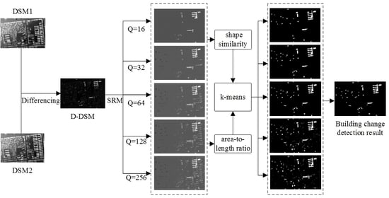
The schedule of the proposed building change detection method is summarized in Figure 2. The approach consists of three main steps: SRM segmentation, shape similarity calculation, and building change detection. The details of each step are described in the following sections.
2.2.1. Segmentation of D-DSM Using SRM
Difference processing is performed on the DSM data at two time instances to generate the difference data D-DSM. Image segmentation is then implemented [25]. First, SRM is conducted on D-DSMs to generate objects, and then the object-oriented building change detection is carried out. In SRM, the observed image X, contains pixels with L bands, and each pixel value belongs to the set (in practice, we would have ). Assuming that X* is the optimal segmentation result, each band value of the pixel in observed image X is obtained by Q-level resampling of each pixel in X*. The pixel value of X* ranges from 0 to g/Q. Q is an independent random variable that tunes the segmentation scale. More objects are segmented as the Q value increases.
SRM mainly achieves image segmentation by iterating between the merging predicate and merging order. The merging predicate can be defined as:
where and denote regions in image X, and denote the average values of band in and , respectively. is formulated as:
where is a constant, and denote the pixel numbers of and , respectively. We set , and denotes the pixel number of image X.
If , and are merged. For the merging order, the function can be used to sort the pixels in X:
where and are the pixels in X, and are the gray values of pixels and in band respectively. Image segmentation can be achieved by simple iteration. The average values of segmented objects are calculated based on D-DSM and a threshold is set for initial change detection. In this experiment, the threshold value was set to 41 (the mean value plus the standard deviation).
2.2.2. Shape Similarity Calculation Using Shape Context Model
Building shapes are usually regular and mostly rectangular. Therefore, the shape context proposed by Ling and Jacobs [26] is introduced to calculate the shape similarity between the changed objects and buildings. It is worth noting that only buildings of rectangular shapes are used to calculate the similarity for changed objects in this test site. If the changed buildings have other shapes, more prior building shapes should be used to generate more accurate detection results. The specific steps of shape context similarity are as follows:
(1) Remove isolated points in changed objects generated by SRM segmentation, and generate sample points in the boundary of objects to represent the shape of the changed objects.
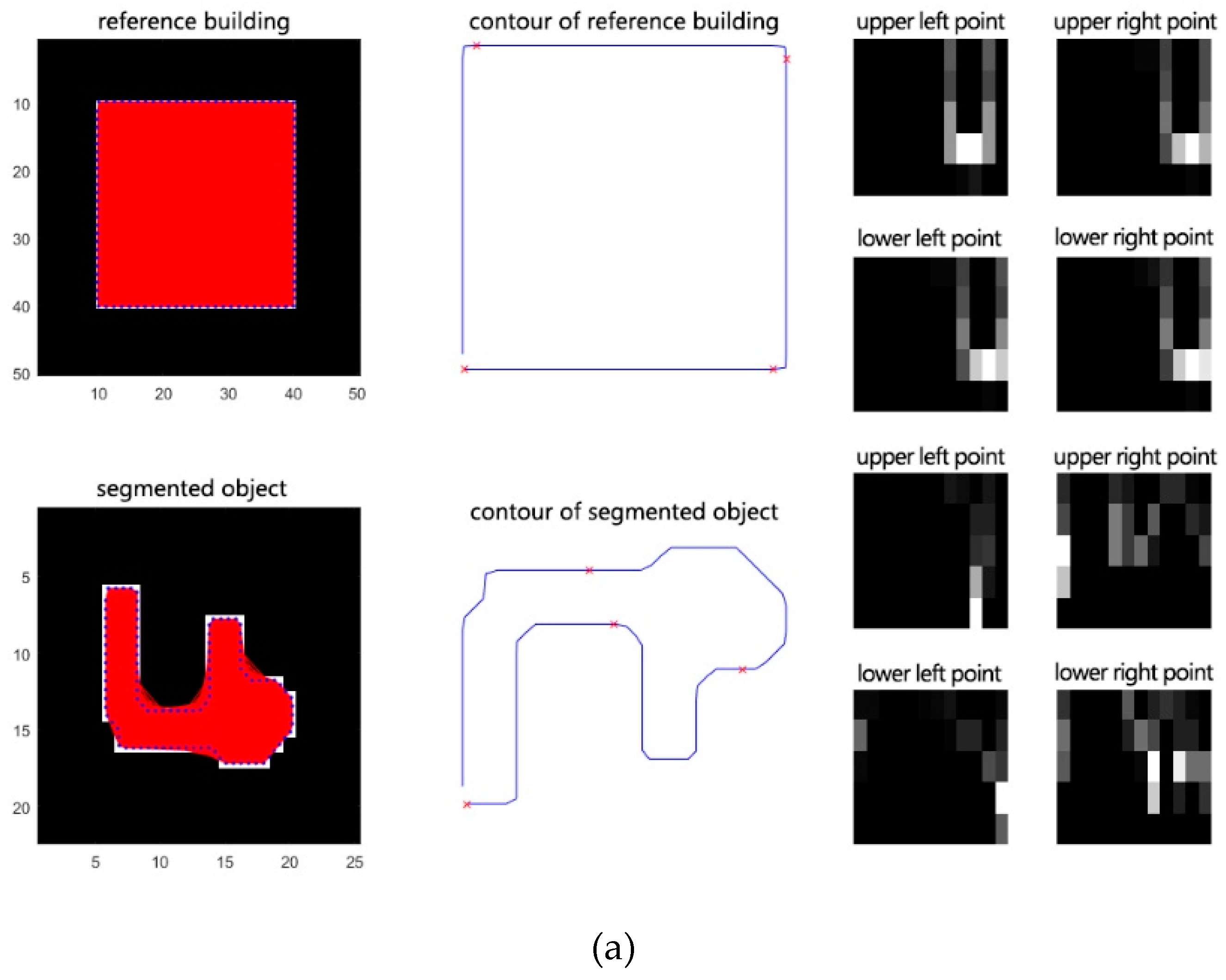
(2) Establish the shape context for all sample points. As shown in Figure 3a, the shortest path between the edge point and another edge point is defined as the inner distance, which is denoted by ; the smaller angle between the tangent at and the inner distance is defined as the inner-angle, which is denoted by . Consider and as a vector, and the point can generate vectors for the remaining points. According to the maximum distance and angle of the vector at point , the inner distance and the inner angle can be divided into and intervals, respectively. For shape point , the histogram generated by its vectors can be calculated as follows:
where , and denotes the number of vectors that fall within the interval. Figure 3b shows the shape of an extracted building, and Figure 3c,d show the shape context histogram of the sample point and sample point , respectively. Finally, histograms generated by points are used to calculate the similarity of the two shapes.
(3) The similarity of the two points can be obtained by calculating the minimum cost of matching the sample point and the sample point . The shape context distribution of the sample points is shown in Figure 3c,d. Let denote the cost of matching these two points. The test statistic can be used to calculate the match cost [27]:
where and denote the histograms at and , respectively, and is the number of histogram bins. The permutation should minimize the total match cost based on sample points:
The dynamic programming algorithm is used to solve the matching problem, and the match cost is used to describe the shape similarity between the shapes of changed objects and the shapes of buildings. For details, please refer to Ling and Jacobs [26]. In general, the larger the number of the shape sample points, the higher the accuracy of the matching results. In this paper, we set .
2.2.3. Building Change Detection Using the K-Means Algorithm
When performing building change detection based on the shape similarity results, the shape of the false detection caused by the miscoregistration of high-rise buildings is very similar to the changed buildings. It is usually distributed around the edge of buildings, which are characterized by a small area and a slender shape, while the changed buildings usually have large areas. Thus, the area-to-length ratio is calculated. The area-to-length ratios are relatively small for registration errors, while the area-to-length ratios of the changed buildings are relatively large.
The k-means algorithm is used to cluster the shape similarity and area-to-length ratio of the changed objects in the initial change detection results. The changed buildings have high shape similarity with building shape and relatively large values of area-to-length ratio, and other changed features have low shape similarity with building shape and relatively small values of area-to-length ratio. The segmented objects are clustered into two types: changed buildings and other changes.
To quantitatively evaluate the performance of the proposed approach for building change detection, three indexes were used to assess the results:
- (1)
- Missed detections (MD): the number of unchanged pixels in the change detection map incorrectly classified when compared to the ground reference map. The missed detection rate is calculated by the ratio , where is the total number of changed pixels counted in the ground reference map.
- (2)
- False alarms (FA): the number of changed pixels in the change detection map incorrectly classified when compared to the ground reference. The false detection rate is calculated by the ratio , where is the total number of unchanged pixels counted in the ground reference map.
- (3)
- Total errors (TE): the total number of detection errors including both miss and false detections, which is the sum of the FA and the MD. The total error rate is described by the ratio .
3. Results and Discussion
The experiments were conducted on a PC with 3.6 GHz clock speed and 16.00 GB RAM. MATLAB 2019 was used to program the proposed method.
In the SRM algorithm, the parameter Q controls the scale of the image segmentation. When the value of Q is larger, there will be more detailed patches in the segmentation results. When the value of Q is smaller, only the objects with a large area can be segmented. We set to analyze the effect of the segmentation scale on the accuracy of the change detection result. Figure 4 shows the segmentation results generated by different Q values. As shown in Figure 4a, when Q = 16, the objects with a large area and a large change value were segmented into independent objects. With the increase of Q, such as Q = 256, more detailed objects were segmented into independent objects. When Q was too small, only the basic objects in the difference DSM data could be segmented into complete parts, and the generated segmentation result was too coarse, which resulted in more missed detection errors. However, it is worth noting that the complete, major and substantially changed objects could still be segmented into independent objects. When Q is too large, there will be more detailed patches in the segmentation result and more false detection errors. For example, for high-rise buildings, the changes caused by registration errors can be detected, which reduces the accuracy of the building change detection results. Therefore, determining the appropriate value of the segmentation parameter Q is essential for generating high-precision change detection results.
On this basis, the shape context was used to calculate the similarity between the building shape and the segmented object. As shown in Figure 5a, when the shape difference between the segmented object and the building was large, the calculated shape context histogram of the corresponding feature points varied greatly. When the shape of the segmented object was very similar to the building, the shape context histogram of the corresponding feature points after calculation was relatively similar, as shown in Figure 5b. Therefore, the more similar the segmented object is to the building shape, the higher the calculated similarity and the smaller the final matching loss will be.
The shape similarity between the segmented object and the building calculated by the shape context is shown in Figure 6. When the shape similarity between the segmented object and the building is greater, it appears brighter in the image, and vice versa. It can be seen from Figure 6 that for segmented objects at all scales, the shape similarity between the major changed buildings and the reference building was high, and the calculated similarity of other changed classes was low. Therefore, when the segmentation scale Q = 32, the shape similarity results could already describe the building changes well. As the segmentation scale increased, more detailed changes were segmented into independent objects, as shown in Figure 6b-e. Especially for high-rise buildings, the changes caused by registration errors were segmented into independent objects, and their shapes were similar to the building shape, as shown in Figure 6 d and e. Thus, it is difficult to automatically extract the changed buildings directly based on shape similarity, especially for the area with high-rise building changes.
Then, the area-to-length ratios were calculated. The area-to-length ratios of the registration errors were usually less than 3, and the area to length ratios of small buildings were usually greater than 6. Therefore, the shape similarity and the ratio of area to length were jointly used to detect building changes.
The k-means algorithm was used to cluster the shape similarity and area-to-length ratio of the segmented objects, and the segmented objects were clustered into two types: changed buildings and other changes. The building change detection results are shown in Figure 7. It can be seen from the figure that when Q = 16, only the buildings with a large area or large changes could be detected. The main reason is that the Q value was too small and the generated segmentation map was rough, resulting in the small buildings not being detected. As the Q value increased, more changed buildings with smaller areas could be detected because the larger Q value generated a finer segmentation map. When Q = 32 and 64, the obtained building change detection result was very similar to the ground reference data, and it could effectively remove the false detected buildings caused by registration. When Q = 256, due to the overly fine segmentation results, there were many false detected changes in the detection results.
Table 1 shows the accuracy of the building change detection results under different Q values. It can be seen from the table that the accuracy of change detection results increased with the increase of the Q value at the beginning. When Q = 32 and 64, the generated building change detection results had a similar total error rate. After that, as the Q value increased, the total error rate also increased. When Q = 64, the kappa coefficient was the highest. Overall, the accuracy of the building change detection results generated at Q = 32 and 64 was generally consistent and more similar to the ground reference data.
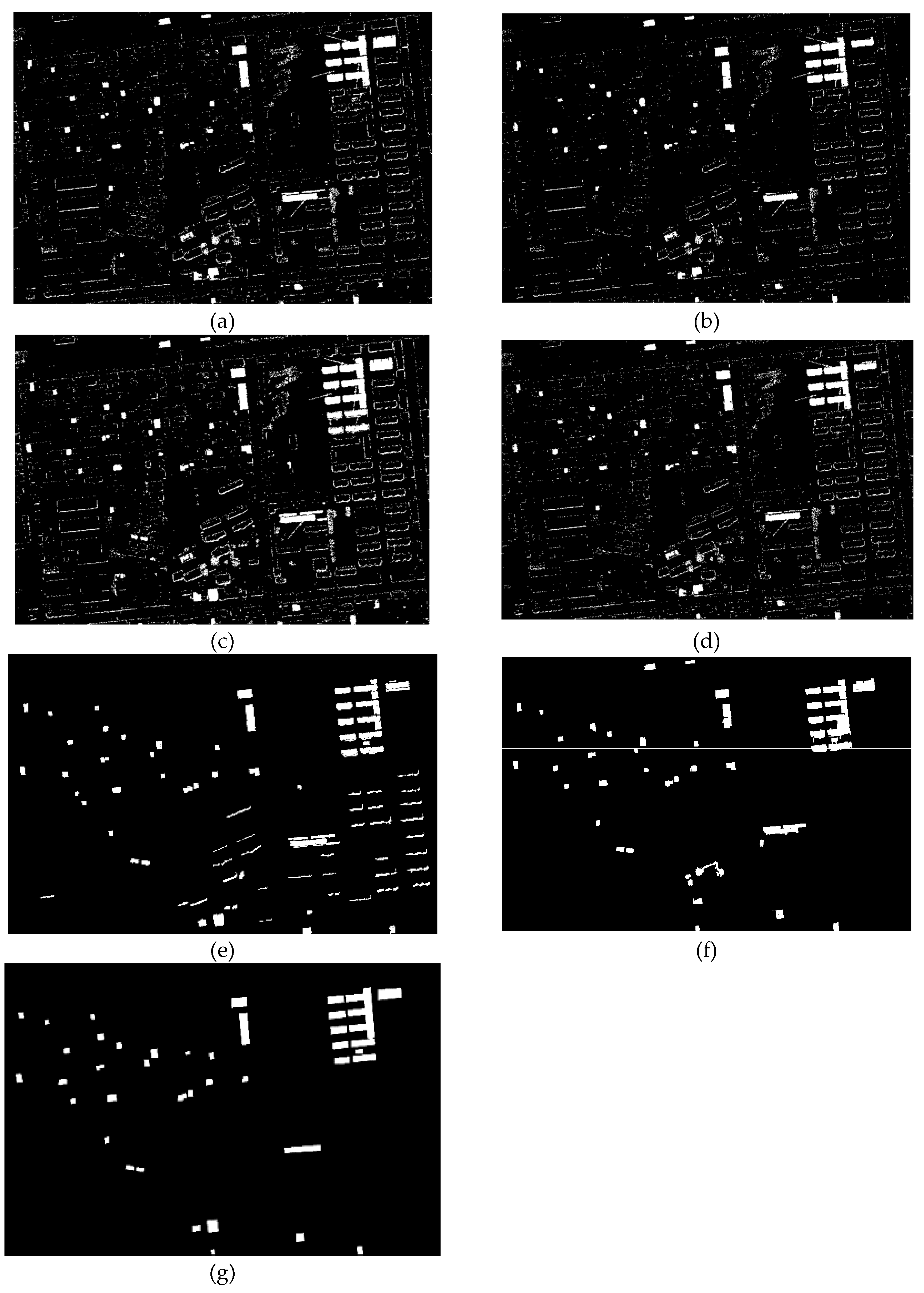
To prove the effectiveness of the proposed method, it was compared with some existing change detection (CD) methods, such as active contour model (CV) [28], multi-scale level set (MLS) [29], MLS+MRF (Markov Random Filed), and fuzzy local information c-means (FLICM) [30], and a building change detection method based on CNN (Convolutional Neural Networks) classification. The results are shown in Figure 8. All the values of the parameter μ, which tunes the length of the active contour, in CV, MLS, and MLS+MRF were set to 0.1, and the value of parameter in MRF, which tunes the balance between spectrum and spatial information was set to 0.5. Figure 8a–d presents the change maps generated by CV, MLS, MLS+MRF, and FLICM, respectively; all of these maps have a large amount of “salt-and-pepper” noise. Figure 8e presents the building change map generated by the CNN classification method, which can effectively suppress noise but have some false alarms caused by the registration errors of high-rise buildings. Figure 8f presents the building change map produced by the proposed method, which is the closest to the ground reference map. The reason is that segmented objects were used instead of individual pixels, and the shape similarity and area-to-length ratio can remove false detection effectively.
Five indices, including missed detection, false alarms, total errors, kappa coefficient, and calculation time were used to quantitatively assess the effectiveness of the proposed method. The quantitative experimental results are shown in Table 2. The missed detection rate Pm, false detection rate Pf, total error rate Pt, kappa coefficient, and calculation time of the proposed method were 16.05%, 0.71%, 1.14%, 0.8, and 29 seconds, respectively. Unlike the other methods used in this study, the proposed method produced the least false alarms and total errors and missed detection levels and calculation time were satisfactory compared with the other methods. Additionally, the proposed method produced the highest kappa coefficient compared with the other methods, which indicates that the building change map has better consistency with the ground reference map. The CNN classification method can achieve satisfactory detection accuracy, but the CNN model training takes a long time.
4. Conclusions
A method for building change detection based on a shape context similarity model was proposed in this paper. First, the difference data D-DSM was generated by the difference processing from the DSM data at two time instances. The difference data D-DSM is then segmented using the SRM algorithm with different scales, and an empirical threshold was set to produce an initial change detection. The shape similarity between the changed objects of the initial change detection result and the buildings was calculated using a shape context similarity model, and the area-to-length ratio for the changed objects was also generated to remove false alarms caused by misregistration. Finally, the k-means clustering method was implemented based on the similarity index and area-to-length ratio to produce a building change map. In the process of segmentation by the SRM algorithm, the change detection results were affected by the scale control parameter Q within a certain range. When the value of Q was 32 or 64, the accuracy of the generated building change detection was almost the same. The SRM segmentation can reduce the “salt-and-pepper” noise caused by the pixel-based method.
The experimental results showed that the proposed method can effectively detect building changes based on DSM data compared with some other popular CD methods. The similarity between the segmented objects and the building calculated by the shape context can effectively extract building changes, and the area-to-length ratio can further remove the false detection changes caused by the registration errors of high-rise buildings and improve the accuracy of building change detection.
However, only rectangular buildings were used to calculate the similarity for changed objects, which may result in missed detections for changed buildings of other shapes. More prior building shapes will be used in future work to generate more accurate detection results.
Author Contributions
Xuzhe Lyu prepared the data and wrote the paper; Ming Hao involved in experiment designing and analyzed the data; Wenzhong Shi reviewed the manuscript and provided comments. All authors have read and agreed to the published version of the manuscript.
Funding
This research was supported by The Hong Kong Polytechnic University, grant number 1-ZVN6 and 4-BCF7; and Research Grant Council, HKSAR, grant number B-Q61E.
Conflicts of Interest
The authors declare no conflict of interest.
References
- Singh, A. Review Article Digital change detection techniques using remotely-sensed data. Int. J. Remote Sens. 1989, 10, 989–1003. [Google Scholar] [CrossRef] [Green Version]
- Bruzzone, L.; Serpico, S.B. Detection of changes in remotely-sensed images by the selective use of multi-spectral information. Int. J. Remote Sens. 1997, 18, 3883–3888. [Google Scholar] [CrossRef]
- Lu, D.; Mausel, P.; Brondízio, E.; Moran, E. Change detection techniques. Int. J. Remote Sens. 2004, 25, 2365–2401. [Google Scholar] [CrossRef]
- Lai, X.; Yang, J.; Li, Y.; Wang, M. A Building Extraction Approach Based on the Fusion of LiDAR Point Cloud and Elevation Map Texture Features. Remote Sens. 2019, 11, 1636. [Google Scholar] [CrossRef] [Green Version]
- Tian, J.; Cui, S.; Reinartz, P. Building Change Detection Based on Satellite Stereo Imagery and Digital Surface Models. IEEE Trans. Geosci. Remote Sens. 2014, 52, 406–417. [Google Scholar] [CrossRef] [Green Version]
- Tian, J.; Chaabouni-Chouayakh, H.; Reinartz, P.; Krauß, T.; d’Angelo, P. Automatic 3d Change Detection Based On Optical Satellite Stereo Imagery. Int. Arch. Photogramm. Remote Sens. Spat. Inf. Sci. ISPRS Arch. 2010, 38, 586–591. [Google Scholar]
- Zheng, Y.; Weng, Q.; Zheng, Y. A Hybrid Approach for Three-Dimensional Building Reconstruction in Indianapolis from LiDAR Data. Remote Sens. 2017, 9, 310. [Google Scholar] [CrossRef] [Green Version]
- Yang, J.; Kang, Z.; Akwensi, P. A Label-Constraint Building Roof Detection Method From Airborne LiDAR Point Clouds. IEEE Geosci. Remote Sens. Lett. 2020, PP, 1–5. [Google Scholar] [CrossRef]
- Murakami, H.; Nakagawa, K.; Hasegawa, H.; Shibata, T.; Iwanami, E. Change detection of buildings using an airborne laser scanner. ISPRS J. Photogramm. Remote Sens. 1999, 54, 148–152. [Google Scholar] [CrossRef]
- Tuong Thuy, V.; Matsuoka, M.; Yamazaki, F. LIDAR-based change detection of buildings in dense urban areas. In Proceedings of the IGARSS 2004. 2004 IEEE International Geoscience and Remote Sensing Symposium, Anchorage, AK, USA, 20–24 September 2004; IEEE: Piscataway, NJ, USA, 2004; 5, pp. 3413–3416. [Google Scholar] [CrossRef]
- Chen, L.; Lin, L.-J. Detection of building changes from aerial images and light detecting and ranging (LIDAR) data. J. Appl. Remote Sens. 2010, 4. [Google Scholar] [CrossRef]
- Stal, C.; Tack, F.; De Maeyer, P.; De Wulf, A.; Goossens, R. Airborne photogrammetry and lidar for DSM extraction and 3D change detection over an urban area – a comparative study. Int. J. Remote Sens. 2013, 34, 1087–1110. [Google Scholar] [CrossRef] [Green Version]
- Rottensteiner, F. Automated updating of building data bases from digital surface models and multi-spectral images: Potential and limitations. ISPRS Congr. 2008, 265–270. [Google Scholar]
- Grigillo, D.; Fras, M.; Petrovič, D. Automatic extraction and building change detection from digital surface model and multispectral orthophoto. Geod. Vestn. 2011, 55, 011–027. [Google Scholar] [CrossRef]
- Malpica, J.; Alonso, M. Urban changes with satellite imagery and LIDAR data. Int. Arch. Photogramm. Remote Sens. Spat. Inf. Sci. ISPRS Arch. 2012, 38. [Google Scholar] [CrossRef]
- Trinder, J.; Salah, M. Aerial images and lidar data fusion for disaster change detection. ISPRS Ann. Photogramm. Remote Sens. Spat. Inf. Sci 2012, 1, 227–232. [Google Scholar] [CrossRef] [Green Version]
- Zong, K.; Sowmya, A.; Trinder, J. Kernel Partial Least Squares Based Hierarchical Building Change Detection Using High Resolution Aerial Images and Lidar Data. In Proceedings of the 2013 International Conference on Digital Image Computing: Techniques and Applications (DICTA), Hobart, TAS, Australia, 26–28 November 2013; IEEE: Piscataway, NJ, USA, 2013; pp. 1–7. [Google Scholar] [CrossRef]
- Choi, K.; Lee, I.; Kim, S. A feature based approach to automatic change detection from LiDAR data in urban areas. Laserscanning09 2009, 38, 259–264. [Google Scholar]
- Matikainen, L.; Hyyppä, J.; Ahokas, E.; Markelin, L.; Kaartinen, H. Automatic Detection of Buildings and Changes in Buildings for Updating of Maps. Remote Sens. 2010, 2, 1217. [Google Scholar] [CrossRef] [Green Version]
- Matikainen, L.; Kaartinen, H.; Hyyppä, J. Classification tree based building detection from laser scanner and aerial image data. Int. Arch. Photogramm. Remote Sens. Spat. Inf. Sci. 2012, 36. [Google Scholar]
- Otsu, N. A Threshold Selection Method from Gray-Level Histograms. IEEE Trans. Syst. Man Cybern. 1979, 9, 62–66. [Google Scholar] [CrossRef] [Green Version]
- Fan, J.; Yau, D.Y.; Elmagarmid, A.K.; Aref, W.G. Automatic image segmentation by integrating color-edge extraction and seeded region growing. IEEE Trans. Image Process 2001, 10, 1454–1466. [Google Scholar] [CrossRef] [Green Version]
- Vincent, L.; Soille, P. Watersheds in digital spaces: An efficient algorithm based on immersion simulations. IEEE Trans. Pattern Anal. Mach. Intell. 1991, 13, 583–598. [Google Scholar] [CrossRef] [Green Version]
- Duarte-Carvajalino, J.M.; Sapiro, G.; Velez-Reyes, M.; Castillo, P.E. Multiscale Representation and Segmentation of Hyperspectral Imagery Using Geometric Partial Differential Equations and Algebraic Multigrid Methods. IEEE Trans. Geosci. Remote Sens. 2008, 46, 2418–2434. [Google Scholar] [CrossRef]
- Nock, R.; Nielsen, F. Statistical region merging. IEEE Trans. Pattern Anal. Mach. Intell. 2004, 26, 1452–1458. [Google Scholar] [CrossRef] [PubMed]
- Ling, H.; Jacobs, D.W. Shape Classification Using the Inner-Distance. IEEE Trans. Pattern Anal. Mach. Intell. 2007, 29, 286–299. [Google Scholar] [CrossRef] [PubMed]
- Belongie, S.; Malik, J.; Puzicha, J. Shape matching and object recognition using shape contexts. IEEE Trans. Pattern Anal. Mach. Intell. 2002, 24, 509–522. [Google Scholar] [CrossRef] [Green Version]
- Chan, T.F.; Vese, L.A. Active contours without edges. IEEE Trans. Image Process. 2001, 10, 266–277. [Google Scholar] [CrossRef] [Green Version]
- Bazi, Y.; Melgani, F.; Al-Sharari, H.D. Unsupervised change detection in multispectral remotely sensed imagery with level set methods. IEEE Trans. Geosci. Remote Sens. 2010, 48, 3178–3187. [Google Scholar] [CrossRef]
- Krinidis, S.; Chatzis, V. A robust fuzzy local information C-means clustering algorithm. IEEE Trans. Image Process. 2010, 19, 1328–1337. [Google Scholar] [CrossRef]
Figure 1.
Experimental data: (a) digital surface models (DSM) obtained in 2017, (b) DSM obtained in 2018, (c) D-DSM, and (d) ground reference map.
Figure 1.
Experimental data: (a) digital surface models (DSM) obtained in 2017, (b) DSM obtained in 2018, (c) D-DSM, and (d) ground reference map.
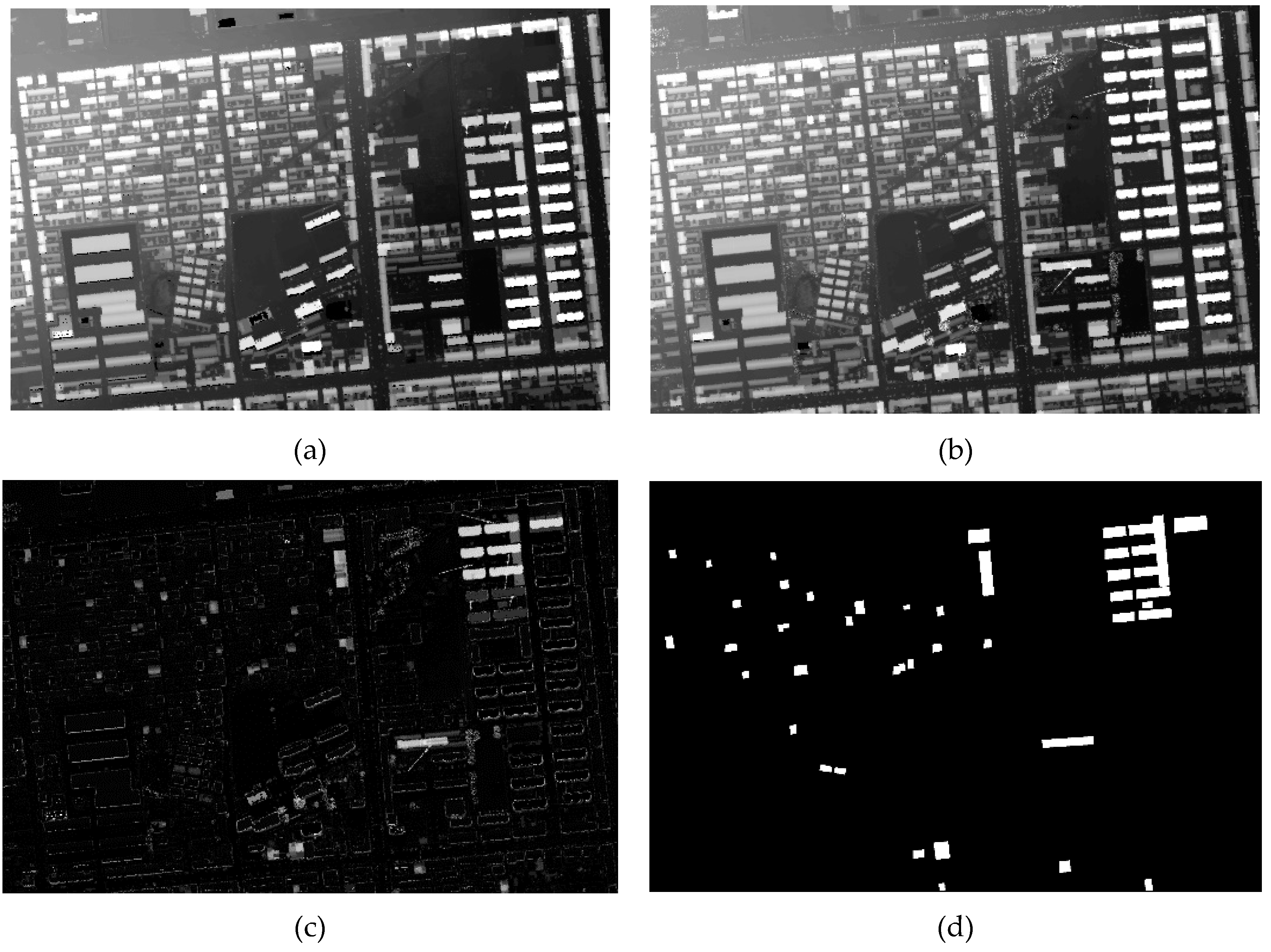
Figure 2.
Schedule of proposed method.

Figure 3.
Establishment of shape context histograms, including (a) the inner-distance and the inner-angle, (b) sampled edge points of a building, (c) shape context histogram of the sample point Z1, and (d) shape context histogram of the sample point Z2.
Figure 3.
Establishment of shape context histograms, including (a) the inner-distance and the inner-angle, (b) sampled edge points of a building, (c) shape context histogram of the sample point Z1, and (d) shape context histogram of the sample point Z2.
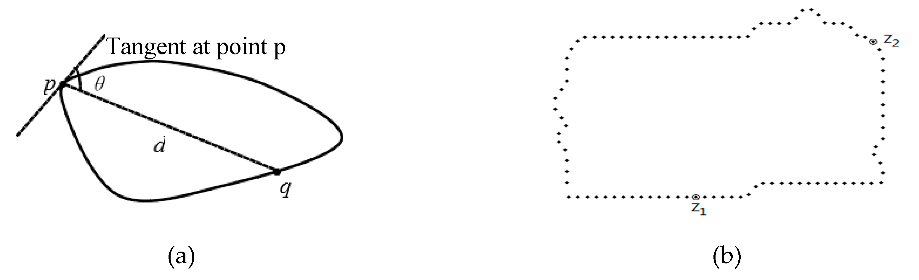
Figure 4.
Segmentation results of statistical region merging (SRM) for D-DSM, including (a) Q = 16, (b) Q = 32, (c) Q = 64, (d) Q = 128, and (e) Q = 256.
Figure 4.
Segmentation results of statistical region merging (SRM) for D-DSM, including (a) Q = 16, (b) Q = 32, (c) Q = 64, (d) Q = 128, and (e) Q = 256.
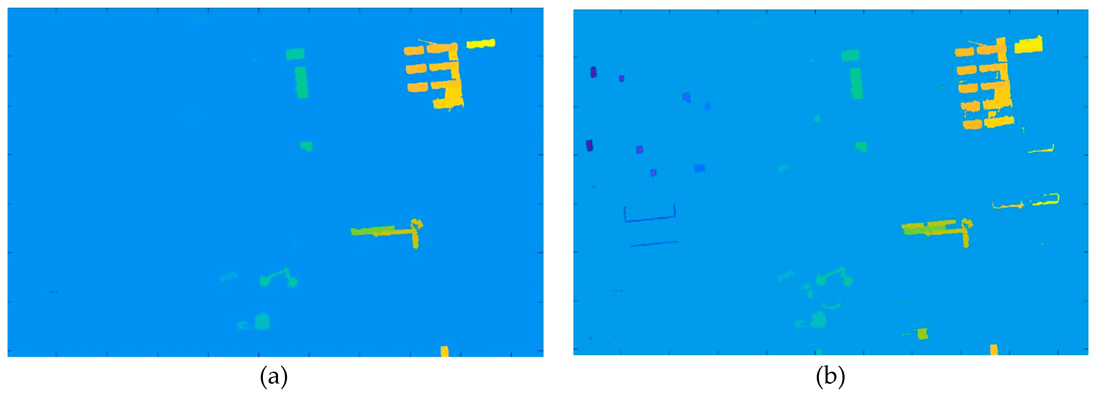

Figure 5.
Shape similarity calculated using shape context: (a) low shape similarity with the building, and (b) high shape similarity with the building.
Figure 5.
Shape similarity calculated using shape context: (a) low shape similarity with the building, and (b) high shape similarity with the building.

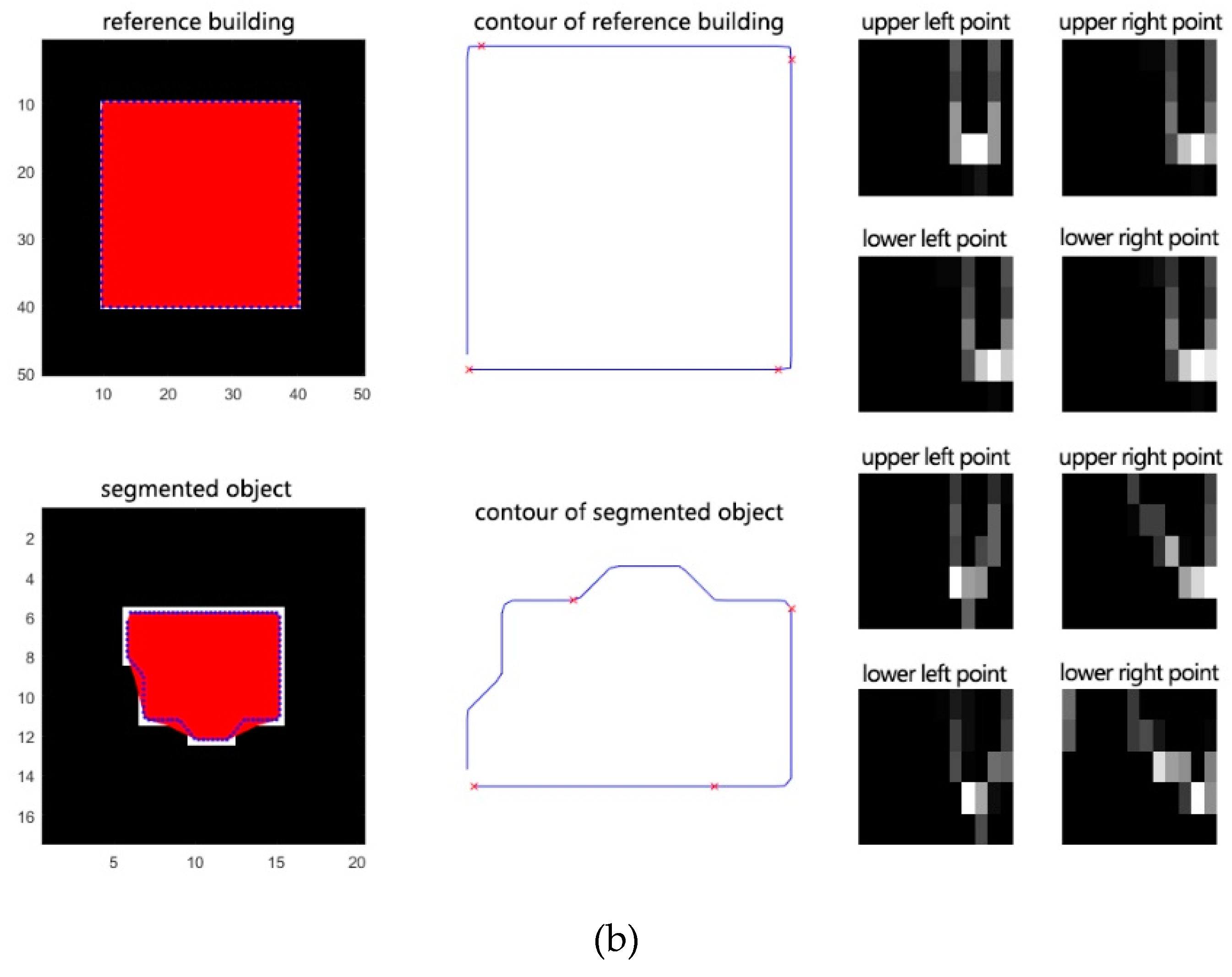
Figure 6.
Shape similarity results under segmentation scale: (a) Q = 16, (b) Q = 32, (c) Q = 64, (d) Q = 128, and (e) Q = 256.
Figure 6.
Shape similarity results under segmentation scale: (a) Q = 16, (b) Q = 32, (c) Q = 64, (d) Q = 128, and (e) Q = 256.
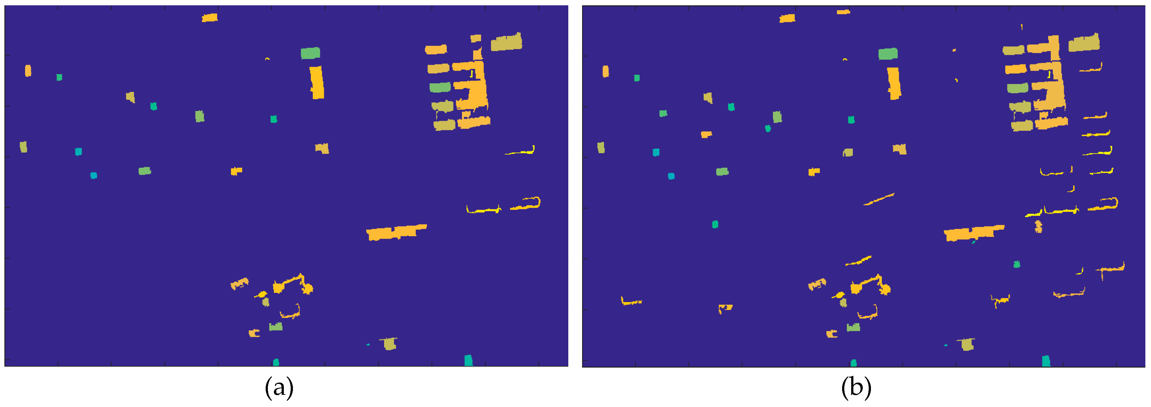

Figure 7.
Building change detection results (white - building changes; black – other changes or non-changes) under segmentation scale: (a) Q = 16, (b) Q = 32, (c) Q = 64, (d) Q = 128, and (e) Q = 256.
Figure 7.
Building change detection results (white - building changes; black – other changes or non-changes) under segmentation scale: (a) Q = 16, (b) Q = 32, (c) Q = 64, (d) Q = 128, and (e) Q = 256.


Figure 8.
Building change detection results (white - building changes; black – other changes or non-changes) compared with popular CD methods: (a) CV, (b) MLSK, (c) MLSK+MRF, (d) FLICM, (e) CNN classification, (f) proposed method, and (g) reference map.
Figure 8.
Building change detection results (white - building changes; black – other changes or non-changes) compared with popular CD methods: (a) CV, (b) MLSK, (c) MLSK+MRF, (d) FLICM, (e) CNN classification, (f) proposed method, and (g) reference map.

Table 1.
Quantitative experimental results under different Q values.
| Q | Missed Detections (No. of Pixels) | Pm (%) | False Alarms (No. of Pixels) | Pf (%) | Total Errors (No. of Pixels) | Pt (%) | Kappa Coefficient |
|---|---|---|---|---|---|---|---|
| 16 | 21,259 | 24.97 | 15,084 | 0.51 | 36,343 | 1.20 | 0.7720 |
| 32 | 14,575 | 17.12 | 19,694 | 0.67 | 34,269 | 1.13 | 0.7988 |
| 64 | 13,662 | 16.05 | 20,776 | 0.71 | 34,438 | 1.14 | 0.8 |
| 128 | 14,369 | 16.88 | 43,610 | 1.48 | 57,979 | 1.91 | 0.6997 |
| 256 | 15,406 | 18.09 | 49,289 | 1.67 | 64,695 | 2.13 | 0.6724 |
Table 2.
Quantitative experimental results compared with popular CD methods.
| Method | Missed Detection (No. of Pixels) | Pm (%) | False Alarms (No. of Pixels) | Pf (%) | Total Errors (No. of Pixels) | Pt (%) | Kappa Coefficient | Time (s) |
|---|---|---|---|---|---|---|---|---|
| CV | 23,865 | 28.03 | 84,947 | 2.88 | 108,812 | 3.59 | 0.5124 | 31 |
| MLSK | 30,319 | 35.61 | 56,454 | 1.92 | 86,773 | 2.86 | 0.5430 | 24 |
| MLSK+MRF | 11,083 | 13.02 | 117,028 | 3.97 | 128,111 | 4.23 | 0.5175 | 52 |
| FLICM | 28,143 | 33.05 | 78,932 | 2.68 | 107,075 | 3.53 | 0.4983 | 17 |
| CNN | 18,642 | 22.39 | 32,735 | 1.21 | 51,377 | 1.84 | 0.7061 | / |
| Proposed method | 13,662 | 16.05 | 20,776 | 0.71 | 34,438 | 1.14 | 0.8 | 29 |
Publisher’s Note: MDPI stays neutral with regard to jurisdictional claims in published maps and institutional affiliations. |
© 2020 by the authors. Licensee MDPI, Basel, Switzerland. This article is an open access article distributed under the terms and conditions of the Creative Commons Attribution (CC BY) license (http://creativecommons.org/licenses/by/4.0/).
Share and Cite
MDPI and ACS Style
Lyu, X.; Hao, M.; Shi, W. Building Change Detection Using a Shape Context Similarity Model for LiDAR Data. ISPRS Int. J. Geo-Inf. 2020, 9, 678. https://0-doi-org.brum.beds.ac.uk/10.3390/ijgi9110678
AMA Style
Lyu X, Hao M, Shi W. Building Change Detection Using a Shape Context Similarity Model for LiDAR Data. ISPRS International Journal of Geo-Information. 2020; 9(11):678. https://0-doi-org.brum.beds.ac.uk/10.3390/ijgi9110678
Chicago/Turabian StyleLyu, Xuzhe, Ming Hao, and Wenzhong Shi. 2020. "Building Change Detection Using a Shape Context Similarity Model for LiDAR Data" ISPRS International Journal of Geo-Information 9, no. 11: 678. https://0-doi-org.brum.beds.ac.uk/10.3390/ijgi9110678
Note that from the first issue of 2016, this journal uses article numbers instead of page numbers. See further details here.