Space-Time Hierarchical Clustering for Identifying Clusters in Spatiotemporal Point Data


1
Measurement and Research, Department of Educational and Psychological Studies, College of Education, University of South Florida, 4202 E Fowler Ave, Tampa, FL 33620, USA
2
School of Geosciences, University of South Florida, 4202 E Fowler Ave, Tampa, FL 33620, USA
*
Author to whom correspondence should be addressed.
ISPRS Int. J. Geo-Inf. 2020, 9(2), 85; https://0-doi-org.brum.beds.ac.uk/10.3390/ijgi9020085
Submission received: 2 December 2019
/
Revised: 17 January 2020
/
Accepted: 27 January 2020
/
Published: 1 February 2020
Abstract
:Finding clusters of events is an important task in many spatial analyses. Both confirmatory and exploratory methods exist to accomplish this. Traditional statistical techniques are viewed as confirmatory, or observational, in that researchers are confirming an a priori hypothesis. These methods often fail when applied to newer types of data like moving object data and big data. Moving object data incorporates at least three parts: location, time, and attributes. This paper proposes an improved space-time clustering approach that relies on agglomerative hierarchical clustering to identify groupings in movement data. The approach, i.e., space–time hierarchical clustering, incorporates location, time, and attribute information to identify the groups across a nested structure reflective of a hierarchical interpretation of scale. Simulations are used to understand the effects of different parameters, and to compare against existing clustering methodologies. The approach successfully improves on traditional approaches by allowing flexibility to understand both the spatial and temporal components when applied to data. The method is applied to animal tracking data to identify clusters, or hotspots, of activity within the animal’s home range.
1. Introduction
Finding clusters of events is an important task in many spatial analyses. Both confirmatory and exploratory methods exist to accomplish this [1]. Traditional statistical techniques are viewed as confirmatory, or observational, in that researchers are confirming an a priori hypothesis. Confirmatory clustering methods attempt to either identify the presence of clustering of lattice or point data or to find the location of these clusters. In contrast, exploratory methods rely on unsupervised machine learning algorithms to identify groups of data in n-dimensional space by using a similarity or dissimilarity metric [2]. Exploratory methods that identify clusters of spatiotemporal data fall under the domain of geographic knowledge discovery (GKD), where the goal is to “discover new and unexpected patterns, trends, and relationships” in the data ([3], p. 149).
In either the case of exploratory or confirmatory, many of the existing methods do not account for time-space or attribute spaces to identify clusters, and are often subject to so-called edge effects tied to the study area boundary [4]. To account for these effects, events closer to the edge are weighted more heavily than those further from the study area edges. This implies there is no explicit consideration of how clustering varies by scale. In addition, the traditional confirmatory methods often fail when applied to newer types of data like moving object data and big data. Mennis and Guo [5] list three reasons why these traditional methods fail with new data: limited perspective or relational model (e.g., linear regression), they were not designed to process the large quantity of information, and they were not designed for “newly [emerging] data types (such as trajectories of moving objects…)” ([5], p. 403).
Moving object data incorporate at least three parts: location, time, and attributes. These attributes may incorporate information about how the agent is moving (e.g., speed, mode, or direction), characteristics of the agent (e.g., age, sex, or income), or environmental/contextual factors (e.g., land use, temperature, weather). The movement of the object might be represented as a sequence of points (such as a trajectory), or distinct events representing known locations of the agent [6]. Although, in the former case, the continuity is created through interpolation between known locations. The idea of the sequence implies a dependence between observations that occur after each other in time. Uncertainty between the locations may be represented as a space-time prism [7,8,9].
If the objects are human agents, then their movement is often tied to existing transportation networks and may be network constrained events [10], that is, events that occur on a one-dimensional space. It has been shown that confirmatory clustering methods overestimate the clustering for linearly constrained point events [11,12,13,14]. This is because the use of a Euclidean distance underestimates the distance between the points. Thus, a network distance metric is preferred [14].
This paper proposes a new space-time clustering approach that relies on agglomerative hierarchical clustering to identify groupings in movement data. The approach, space–time hierarchical clustering, incorporates location, time, and attribute information to identify the groups across a nested structure reflective of a hierarchical interpretation of scale [15]. These three components are combined using weighted linear combination to create a modified distance metric. Each of the components are constrained through a scale factor. The method is developed for studying observations of discrete point events that may occur on and off of a network. The purpose of this new approach is to account for the cyclical nature of time, while incorporating physical distance, and the potential of viewing clusters at multiple temporal and spatial scales; which are not well accounted for in existing approaches. Emphasis is given to points representing repeated observations for a given period, such as the 24-h cycle of a day. Simulations are used to understand the effects of different parameters, and to compare against existing clustering methodologies. Finally, the method is applied to animal tracking data to identify clusters, or hotspots, of activity within the animal’s home range.
The paper is organized as follows. The next section discusses existing clustering algorithms and their limitations for spatiotemporal data. Particular emphasis is given to hierarchical clustering since this is foundational for the rest of the paper. Section 2 presents the distance metric for the hierarchical clustering algorithm and discussing each of the components separately. Section 3 discusses simulations used to estimate the different parameters in the distance metric and compares space-time hierarchical clustering to potential alternatives. Finally, the new approach is applied to animal tracking data and the results are discussed.
1.1. Background
Spatial data mining, or more generally GKD, is a subdiscipline of data mining and machine learning that focuses on the exploration of spatial and spatiotemporal data – specifically, the massive amount of fine resolution data derived from location-based services, real-time data, volunteered geographic information (VGI), or remote sensing [1,16,17,18]. Geographic knowledge discovery focuses on developing methods to handle this specialty data, with the goal of knowledge extraction. The broad domains include: segmentation or clustering, classification, spatial association rule mining, deviations, trends, and geovisualizations [3,5].
Often, the data for GKD will be messy, and the first step towards knowledge extraction will be to filter or clean it. The location may be prone to measurement errors either through the mobile device’s GPS or cellular network-based location [18,19]. Different steps for filtering or cleaning this may be to convert, or aggregate the locations to a significant place, or as Ashbrook and Starner [20] phrase it, a place where “a user spends her time” ([20], p. 278). A significant place’s time interval does not have to be over days but a few minutes. Andrienko et al. [21] use the idea of a stop to define a significant place: “a place significant for a person can be recognized from the number and duration of stops” ([20], p. 10). A stop is a location where an agent stays for a certain duration. It is “manifested by a temporal gap between consecutive position records” ([21], p. 10).
1.2. Common Clustering Techniques
Clustering “is the process of grouping large data sets according to their similarity” ([22], p. 208). The two defining characteristics of any clustering analysis are determining the measure of similarity (or dissimilarity), and the algorithm used to identify the clusters. There are several measures of similarity that calculate the distance between observations, but Euclidean distance is the most common [23]. Exploratory methods of spatial clustering of point data fall into four categories: partitioning methods, hierarchical methods (agglomerative or divisive), density-based methods, and grid-based methods [22]. It is important to separate the conceptual task of clustering from the algorithms and measures of similarity used to achieve that task [23]. There are a multitude of algorithms used to achieve hierarchical clustering that may use the same or different methods of measuring similarity. The different clustering methods and common algorithms are summarized in Table 1.
A limitation with several of the clustering algorithms listed in Table 1 as applied to spatial data is that they do not necessarily account for the boundaries of the region, or spatial constraints [24]. This means that clusters generated from the spatial data may not be proximate or contiguous. Guo [24] defines regionalization as a “special form of clustering that seeks to group data items…into spatially contiguous clusters…while optimizing an objective function (e.g., a homogeneity measure based on multivariate similarities within regions)” ([24], p. 329). This is further complicated when there are two components that need to be integrated into the cluster with different boundaries: a physical/spatial boundary and a temporal boundary. The time difference, and temporal boundary, between the two events will depend on the application. Clustering that incorporates both space and time traditionally use a metric that identifies both spatial and temporal similarity [25].
There are various proposed approaches to incorporating temporal information. Birant and Kut [22] in their space–time extension of the density-based spatial clustering of application with noise algorithm (ST-DBSCAN), use a filter to measure the distance between neighbors only if they occurred consecutively, depending on the timescale (years, days, hours, etc.). They also separate the spatial and “non-spatial” information into two separate distance calculations to define the neighborhoods that generate the groupings [22]. Wang et al. [26] also use a neighborhood searching to adapt the DBSCAN algorithm (also called ST-DBSCAN), as well as an ST-GRID approach. Agrawal et al. [27] adopt a similar approach in their space-time extension of the OPTICS algorithm (ST-OPTICS).
In some cases, the spatial distance is weighted by the temporal component [25,28]. In other cases, space and time is combined to form one spatiotemporal distance. Andrienko and Andrienko [29] method “proportionally transforms t [time] into an equivalent spatial distance,” and then uses Euclidean distance to combine the two ([29], p. 19). Oliveira et al. [30] adapted the shared-nearest-neighbor (SNN) density-based clustering approach to incorporate space-time, and non-spatial information by using a weighted combination of the three components (SNN-4D+) [31]. Other approaches have been developed that specifically target trajectory clustering rather than discrete events (see for example Lee et al.’s [32] trajectory clustering (TRAJCLUS) algorithm), or for measuring the similarity of trajectories [33].
Common to each of these methods discussed above is how these algorithms approach time. Typically, it is viewed as a linear, increasing function, so that the difference between two time events can be calculated. Of course, there are different ways to view time, such as cyclical or as the time of day. Often, time’s inclusion appears to be an afterthought to these methods. Time distance should be adaptable. They also do not contend with data that is network constrained, and use Euclidean distance for their calculation, although Manhattan distance could be substituted. Euclidean distance is the classic straight-line distance (as the crow flies), and Manhattan attempts to adjust for distances within a network.
Agrawal et al. [27] also provide several requirements for clustering of space-time data. The methods should be able to identify groups with arbitrary or irregular shapes. They should be able to manage high dimensional data and be scalable (in terms of computing power). Not surprisingly, they should have the “ability to deal with spatial, non-spatial and temporal attributes;” which also implies that they should be able to add and remove each of these components as needed ([27], p. 389). As Guo [24] also suggests, they should be able to manage nested and adjacent clusters, independent of the order of which they are entered into the algorithm. Finally, in order to be useful, the results should be interpretable. In addition to these, this research also suggests that incorporating a notion of scale into the analysis is important, particularly for the nested clustering. This can be done with a hierarchical clustering approach.
1.3. Hierarchical Clustering
Hierarchical clustering is divided into agglomerative and divisive techniques, depending on whether the approach is to start from the bottom with individual observations considered each as a cluster then aggregated, or the top with all observations considered as one cluster then divided. In the agglomerative approach, there are at least four methods of merging clusters: single-linkage, complete linkage, average group linkage, and centroid linkage. Single-linkage defines the distance between groups as the distance between the nearest cluster members. Complete linkage methods use the furthest distance between members of clusters. Average group linkage takes the average of the distances between members of clusters, or the weighted average might be used (Ward’s method is an example of this). Another approach uses the centroids of the cluster to measure the distances between them [2]. The average approach, also known as unweighted pair group method with arithmetic mean (UPGMA), is appropriate when using a custom distance metric that will be defined below [34]. This method takes the (weighted) average of the distances between members of clusters as shown in Equation (1). In this equation and are two different clusters, while are members of the cluster, and is some distance function.
2. Proposed Approach
2.1. Space–Time Hierarchical Clustering with Attributes
Space–time hierarchical clustering uses a specific linear weighted combination of spatial distance, temporal distance, and attribute distances that are discussed in more depth below. These distance calculations are used by the traditional hierarchical clustering algorithm to identify clusters. The proposed space–time hierarchical clustering approach presented here meets the basic requirements set out by Agrawal et al. [27]. A flexible approach is adopted, which allows for different conceptions of spatial distance and temporal distance to easily be incorporated into a single distance metric. By modifying only the distance metric () instead of developing a new algorithm, the method can easily be ‘plugged’ into existing algorithms such as those listed in Table 1, although hierarchical clustering is selected for this paper. This existing algorithm is selected so it is easier to use in existing software. The choice of an agglomerative hierarchical is selected for two reasons: there is no requirement for pre-selecting the number of clusters, and it easily brings in the notion of hierarchical scale, and ability to view clusters (and nested clusters) across different levels. The new distance metric used for hierarchical clustering is a weighted linear combination of spatial and temporal distances, and non-spatiotemporal attributes or variables. While similar conceptually to the approach adopted by Oliveira, Santos, and Moura Pires [30], there are several modifications to the weighting, scaling, and handling of the spatial and temporal components.
Given two clusters (or observations), and , their similarity is measured by the combination of their location in time and space, and any external variables, as shown in E2. Each component is handled with a different distance calculation, then normalized and weighted before adding together. The distance function, , calculates the distance between the two locations represented as vectors and (simplified notation of x and y point coordinates). The distance between the locations is scaled, or normalized, by and given a weight, . The scale factor is the minimum distance to be considered as related, and the weight is emphasis put on a particular component. The temporal distance between the clusters is calculated by the function , and does not assume a linear difference between and . This temporal distance is scaled by , and given a weight of . Assuming the potential for a high dimensional set of non-spatiotemporal variables, the last component is the summation of the attribute distance for multiple attributes from a to q. Each attribute distance is scaled by a different factor, , depending on the type of variable (although it is assumed to be numeric), and each attribute is given a weight of . Once each component is added together, it is divided by the sum of the weights.
Equation (2) is purposefully general so that each of the distance functions (, , and ) can easily be adapted to fit different types of data. The spatial distance metric may accept Euclidean distance, or a network distance for network constrained or mixed events, or other metrics. The temporal distance may contend with linear or cyclical time. Each of the distance functions will be explored in more depth in the next sections. The subindex a refers to the index of the weight, and for attributes the weights will begin after 2 and increase for every new attribute.
2.1.1. Calculations for Distance
For point events defined in a two-dimensional planar space, distance may be calculated by the Euclidean distance between two events with and coordinates, as shown in Equation (3). As discussed above, using planar distances for points constrained to linear networks overestimates the clustering [11,13,14]. It is common for moving object human data, whether it be trajectories or discrete known locations, to be affected by the transportation network (e.g., motor-vehicles crashes on a street network). In these cases, network distance is based on the segment lengths of a physical transportation network. Realistically, however, human movement will be a mixture of network constrained locations and two-dimensional planar locations. Thus, distance should be able to contend with this mixture.
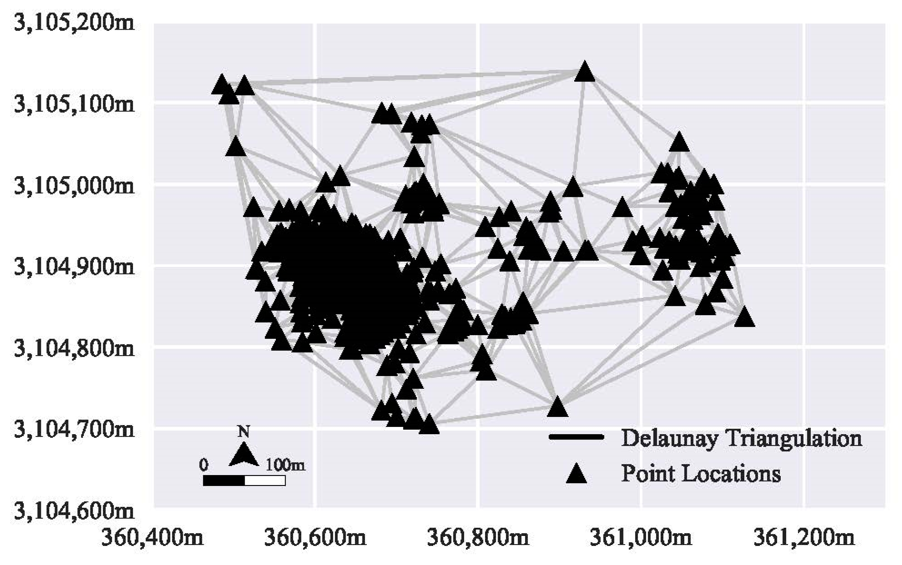
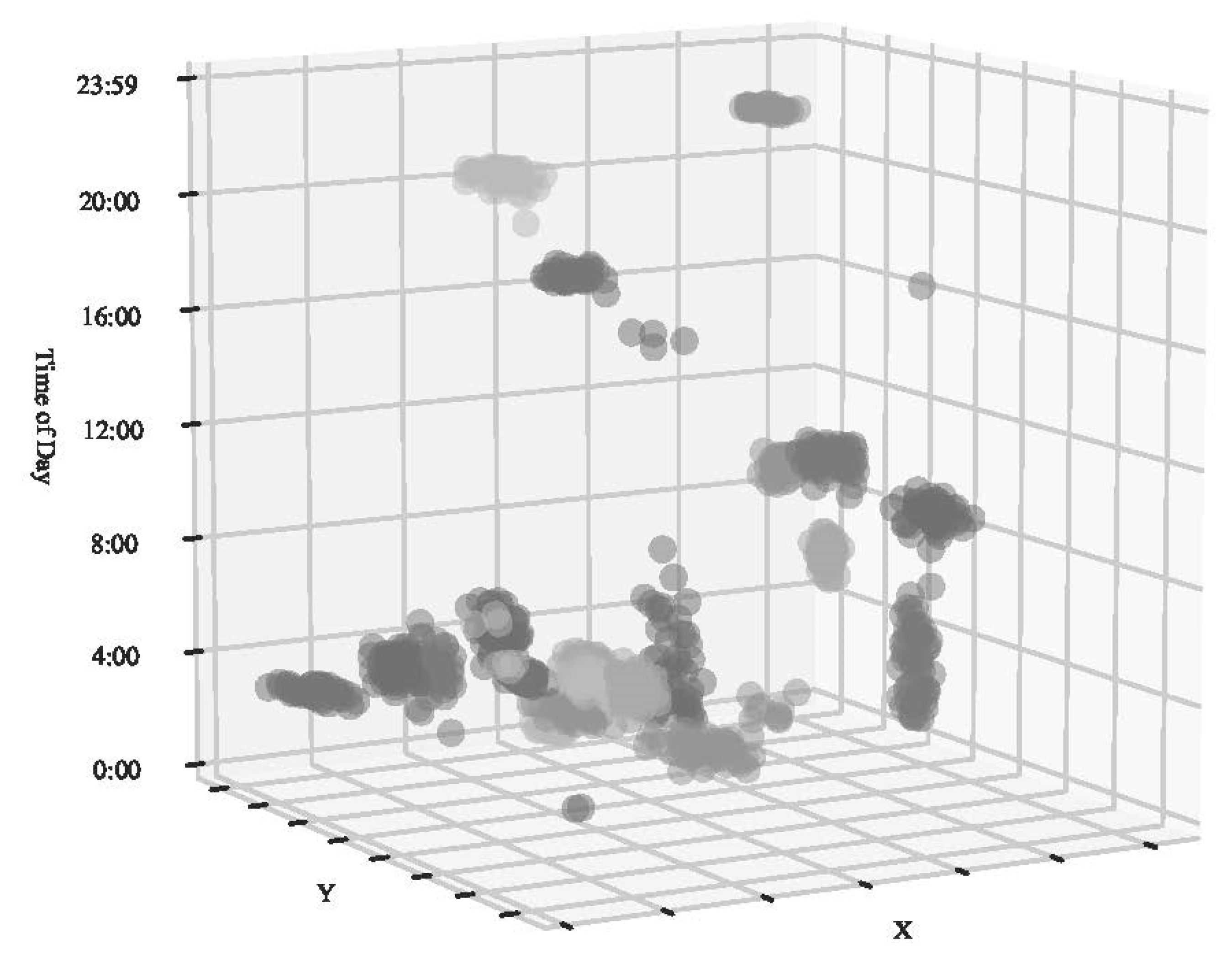
One way to manage this mixture of network constrained data and free flowing data is to develop a network around the unique locations in a set of point observations. To do this a neighborhood graph is developed from the set of points (P). Ideally the, the neighborhood graph will reflect the movement patterns of agents between known locations [35]. This means that the connection, or edge, between the points reflects the route the agent took to reach that point. One common neighborhood graph is the Delaunay triangulation (DT), which tessellates space into a series of connected triangles [36]. This is done for the set of P points such that no point is inside the circumcircle of any of the triangles in the plane [37]. The DT represents a rigid neighborhood structure. Figure 1 presents a DT for a set of animal tracking data, potentially reflecting the pathways the animal may follow given a sequence of points [35].
To calculate the distance for either a physical transportation network, or a network derived from the neighborhood DT structure, the network should be converted to a graph data structure. Where a graph, , is defined as a set of nodes (Equation (4)) and a set of edges (Equation (5)) such that [38,39]. Edges are subsets of node pairs, defining the start and end nodes as shown in Equation (5). Each of these node pairs are assigned a property or weight, such as the physical distance between the features a node represents.
A path on a graph from node and is a sequence alternating nodes and links as shown in Equation (6) [38]. A common path of interest is the shortest path between nodes, and may be calculated using algorithms such as Dijkstra or A* [39,40]. Using this path approach, the distance between to nodes , is the shortest path between them, .
The weighted linear combination shown in Equation (2) would accept either the planar distance, , or network distance, . Once the distance is calculated, it is scaled by . This serves two purposes: to eliminate the units to place the distance on the same scale as the other components, and to create spatial constraint so that clusters are nested and address Guo’s [24] point regarding regionalization.
There are several options to pick the scaling value, , for the distance component. For example, various fixed values may be selected such as the maximum distance between all points in the dataset, or the total network length if using a network distance. Oliveira et al. [30] suggest taking the distances from the lower left corner of the boundary of the study area and visualizing it to select the difference.
Alternatively, an adaptable distance could be used. In this case, changes for each cluster, . For this research is set using the maximum distance of the nearest neighbors of . This creates irregularly shaped clusters that adapt depending on how far away is from the other clusters. If only the spatial component is used (, then the clusters are spatially nested within each other based on the agglomerative hierarchical clustering. Equation (7) shows the set of distances for a cluster, , ordered by distance. The maximum of these values then becomes for a particular . If the distance between and is greater than (the scale factor), then this component will be greater than 1. In essence, the scale factor can be interpreted as how far apart two events should be considered as near each other.
The selection of how many neighbors to use, , is difficult. Local knowledge of the dataset may be used to set this parameter. In similar instances, the heuristic of using the natural logarithm of the number of observations could be used to determine a starting value for k [22,41]. Simulations are used below to explore this option.
2.1.2. Calculations for Time
The second component in Equation (2) is that of time, made up a distance function, , and scale factor, . The temporal distance function could take several forms depending on how time is considered. For example, with a cyclical view of time interest is not so much that the event occurred exactly near each other in time, but that the pattern of occurrence is similar. That is, two events occurred during the same part of the day and potentially months apart. This is applicable in identifying a significant place from an agent’s repeated patterns of use at particular times of day. Other views of time may be that two events occurred temporarily proximate (same year, month, day, and hour).
In the second case, temporal proximity is whether the events occurred within a certain time frame from each other. This is a simple difference between and . Closer events will have a smaller difference. Equation (8) presents one case of the absolute difference in time which is the total amount of time difference between two events. For example, the result may be the total seconds, or other unit dependent on the type of time values that are associated with a moving object.
The scale factor, , when considering the temporal distance, will constrain temporal values to be more similar within a time frame. For example, scaling all values to one hour will make absolute differences less than an hour within one, or greater than one if over an hour. The scale factor should be in the same units as . The scale factor plays the same role as with the spatial distance. It constrains, and also places time on the same range of values as the spatial and non-spatial distances.
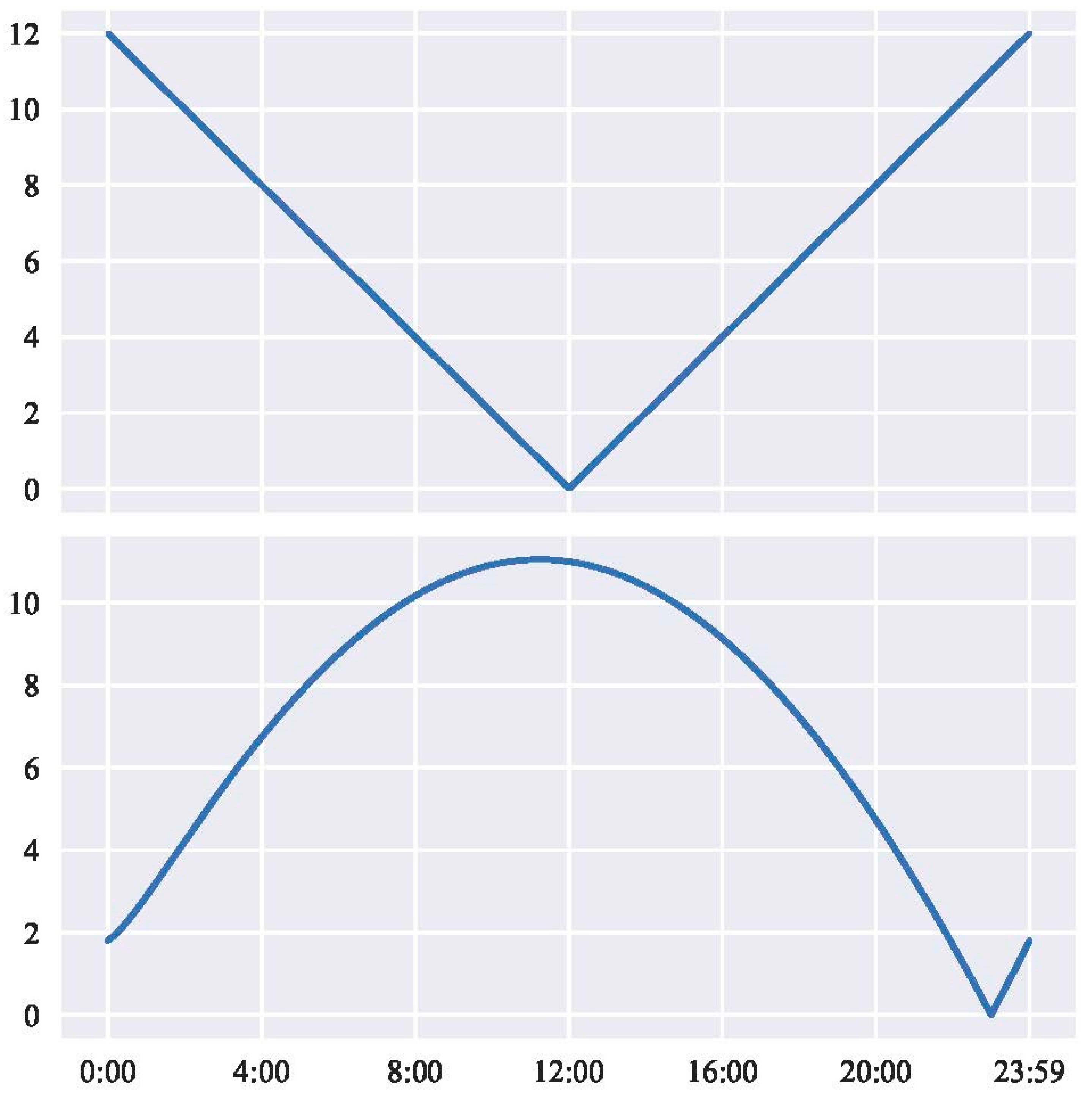
In the case of repeated patterns, each event’s timestamp needs to be placed on the same timeline. This is easily done by placing the event on the same linear scale as the number of seconds from midnight. However, this treats times at midnight (0 h) and close to midnight (23 h) further apart. Realistically, an event at these times would be more similar than those between 0 h and 12 noon. To compensate for this similarity problem, the difference between event times is transformed to fit a curve. This forces the difference between time at the end points (0 h and 23 h 59 min) to be closer in value. This is shown in Equation (9), where and T are defined in Equation (10), assuming the timeline is seconds from midnight otherwise T would have a different value. Each event’s time value, and , is centered around (43, 200 s), absolute difference is taken. The result of this difference is scaled to radians. The results of are between 0 and 1. This value can be converted back to the Euclidean space using the law of cosines as shown in Equation (11) giving the value for .
The scale factor, , is applied in the same way as the scale factor for distance, but should be in the same units as the time value (seconds for example). To constrain the temporal distance to one hour, use a value of 3600 s. The result is which places values within an hour to be less than one, and greater than an hour’s difference to be greater than one.
Figure 2 presents two examples of how the temporal distance between 23 h or 12 h and every other time in seconds from midnight. Note the distance result in is shown on the y-axis. The v-shape at the top panel in Figure 2 shows how distance from 12 h (noon) is at the maximum closer to midnight (0 h). In contrast, at 23 h, the distance is farthest at noon, but decreases closer to 0 s from 23 h and 86,400 s from midnight. In Figure 2, the sharp V-shape at the bottom panel indicates a distance of 0.0 at 23 h. The different shapes of the curve will change depending on what the center-point will be (v-shaped at 12 h and curved at 23 h). This is due to the conversion of time using the cosine function.
2.1.3. Calculations for Attribute Space
Non-spatial or temporal information may be further used to define the cluster. The distance, , will may be a simple absolute difference between the values. This is scaled by, , to place the attribute values on the same measurement scale as distance and time; nearer events will have a value of less than 1 and far events will be greater than 1. The maximum value of the variable, or other relevant statistic, could be used to scale it. In the case of a binary value, the only scenario of difference is when one of the inputs equals 1 and the other is 0, when scaled by 1 it equals 1. Every other case results in 0. The choice in function will depend on the variable.
2.1.4. Implementation
Equation (2) was implemented in Python 2.7 using the SciPy and NetworkX packages [42,43]. A custom distance function created a distance matrix between events for Equation (2). Network distance was calculated as the shortest path between two nodes using Djikstra’s algorithm, as implemented in NetworkX. The Delaunay triangulations calculated for the point datasets was created using the SciPy library. The hierarchical clustering algorithm used average linkages to develop clusters.
2.2. Relation to Spatial Scale
A primary reason for rooting the space-time analysis in hierarchical clustering is because it incorporates a view of scale as a nested hierarchy. Within this view, spatial and temporal scales are nested, creating larger groupings of observations along a vertical axis. The hierarchical view of scale is not new, particularly amongst biophysical geographers [44]. For example, Levin [45] proposed his hierarchy theory as an explanation of scale in natural systems and ecology. Hierarchy theory also implies a view that spatial and temporal scales covary. In many ways, this covariation is reflected in the space–time hierarchical distance that combines both components. In addition, attribute space may covary with the other components.
As with other spatial analyses, the modifiable areal unit problem (MAUP) notes that the results of an analysis will vary depending on the resolution of the spatial data (e.g., census blocks versus census tracts) [46]. Also, according to the uncertain geographic context problem (UGCP), the context of the phenomena under study will vary across different scales [47,48]. The space-time hierarchical clustering methodology will be affected by the overall spatial and temporal boundaries of the study area, but also has the flexibility of choosing and evaluating the clusters across different hierarchies or levels.
The choice of level is difficult to determine when the number of clusters are not known a priori (as is the case in the ground truthing simulations). However, at least three different approaches are available: empirical, fit, and operational. Empirical suggests an evaluation of the dendrogram to determine a level that is appropriate for evaluation, or identifying the number of clusters that could be useful for understanding the phenomena. For determining the number of clusters based on fit, a metric such as silhouette score could be used to determine which level provides the best score out of all levels. Finally, operational scale “refers to the logical scale at which a geographical process takes place,” and thus a level for the clusters based on knowledge of the processes that may have generated them ([44], p. 5).
3. Results
3.1. Simulations
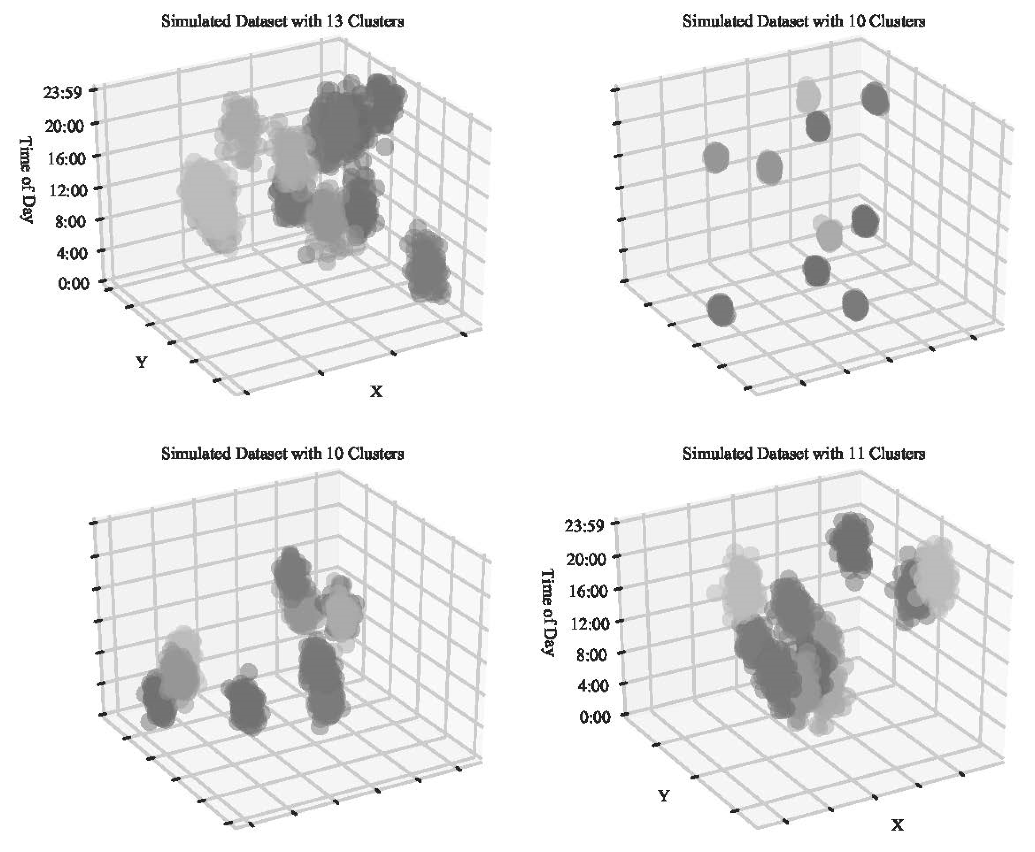
In order to evaluate the influence of the nearest neighbor parameter and the choice of the temporal scale factor, fifty simulated datasets were generated. These were created using three variables: an x coordinate, y coordinate, and temporal variable simulated as seconds from midnight. Each variable used a standard deviation randomly selected from a uniform distribution between 1000 to 7000. The number of clusters generated for each simulation was randomly selected between 5 and 20 whole numbers. The centers for each cluster was also randomly selected from a uniform distribution of 500,000 to 780,000 for x coordinates, and 370,000 to 500,000 for y coordinates (reflective of the Universal Transverse Mercator zonal system). The temporal variable was randomly selected from a uniform distribution from a base of two times the randomly selected standard deviations to 86,400. This bottom value was chosen to avoid any values below 0. The make_blobs function part of the Sci-Kit Learn package was used to generate these simulated clusters [49]. A total of 1000 observations were generated for each simulation. Four of the simulations are presented in Figure 3. The variation in the standard deviation can be seen in the different figures, with some clusters spread out with some overlap, and some tightly constrained.
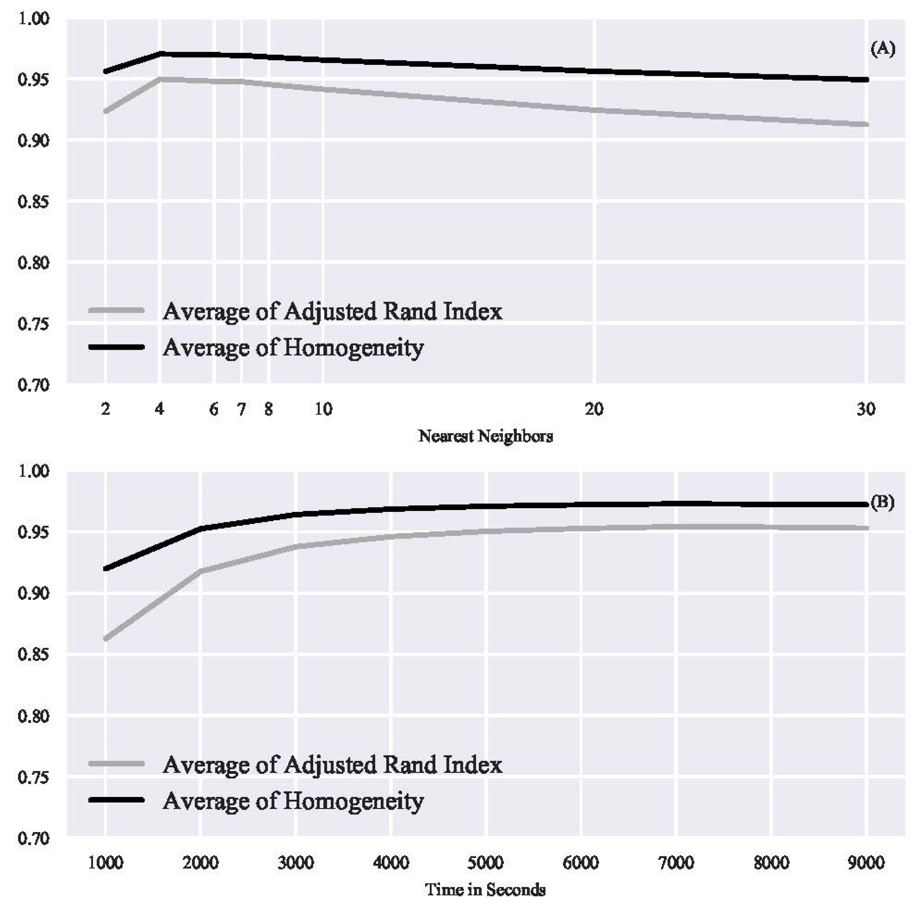
The space-time hierarchical clustering algorithm was applied to each simulation for different choices of (2, 4, 6, 7, 8, 10, 20, and 30) and (1000 to 9000, by 1000). Distance was calculated as network distance using a DT. To evaluate the best fit for each of the variables two performance metrics were used: homogeneity score, and average random index score [50,51]. These performance metrics compare the cluster assignments to a ground truth such as the original cluster label. The homogeneity score ranges from 0 to 1, with 1 being perfectly homogeneous, meaning all the clusters only contain observations of the same group. The adjusted random index score ranges from −1 to 1 with 0 being completely random assignment, and 1 being a perfect match to the ground truth clusters.
Figure 4 shows the average homogeneity score and average adjusted random index score for different values of and . In Figure 4A, the average scores are for different values of the nearest neighbors averaged across the different values of . There is a slight bend where performance improved between 4 and 10 nearest neighbors, then decreased for smaller values, 2, and larger values, >20. In Figure 4B, the average scores are for different values of the temporal scale averaged across the different values of . Performance improved to about 3000 s, but then leveled off, and there was not much improvement after that value.
Also considered was the highest score for a combination of and . The average of these for the adjusted random index score was a nearest neighbor of 6.9 (standard deviation of 7.4), and average temporal scale of 3490 (standard deviation of 2968). The average of and for the maximum homogeneity score was 6.8 (standard deviation of 7.2) for the nearest neighbor parameter, and 3607 (standard deviation of 3059). As suggested before, the natural logarithm heuristic might be used to determine the nearest neighbor parameter. The natural log of the sample size, 1000, is 6.9. In the case of most of the simulations, a value of 7 would have worked well. The temporal scale factor suggests a value of approximately 3600. This is one hour in seconds. This latter scale factor may be better set given external knowledge (e.g., using the average velocity of the object moving to understand the temporal range of the object).
3.2. Comparison with Alternative Clustering Approaches
To better understand the space–time hierarchical clustering approach, the results of applying it to a simulated dataset were compared to two other methods: Euclidean based hierarchical clustering, and ST-DBSCAN. The traditional hierarchical clustering (see Section 1.3) method is used to compare how the proposed space-time hierarchical clustering approach performs on spatiotemporal data to a naïve approach. ST-DBSCAN is a density-based algorithm for clustering spatiotemporal data based on certain parameters [22,52]. The approach for the ST-DBSCAN are different from hierarchical clustering in at least two ways: it reduces the noise in the data, and it automatically detects the number of clusters within the dataset.
The dataset was created as above, with twenty clusters and a sample of 1000 and 20 clusters. The spatial variables are randomly distributed cluster centers along the x and y coordinates, with a randomly selected standard deviation between 1000 and 7000. The temporal variable was simulated to reflect the nature of cyclical data. The center was randomly selected, but if the distribution fell over midnight (86,400 s) then it was switched to +0:00. The data is presented in Figure 5. In some cases, at the top of the z-axis (time), the cluster is split between midnight and 23:59.
The ST-DBSCAN requires a spatial threshold, which is a cutoff point for the spatial component, and temporal threshold, a time value cutoff. The latter is similar to the time scale in the space-time hierarchical clustering and the same value was used for both (1 h, or 3600 s). The space-time hierarchical clustering parameters were selected based on the simulation studies presented in Figure 4 (natural log of the sample size, and 3600 for the time scale). We compared the same parameter settings for the space-time hierarchical clustering and ST-DBSCAN, and then iteratively changed the parameters for ST-DBSCAN. One problem with the ST-DBSCAN in making direct comparisons is the number of clusters identified. Hierarchical clustering in general lets the user pick the number of clusters, whereas ST-DBSCAN identifies the number of clusters from the data, plus noise. When the same parameters were used for both approaches, ST-DBSCAN could only find 15 clusters and noise in the dataset. To better compare the two approaches, 15 clusters were selected for the space-time hierarchical clustering, and an iterative approach was used to identify better parameters for the ST-DBSCAN. Combinations for minpts (1 to 30), spatial threshold (1000 to 100,000), and temporal threshold (1800, 3600, 7200 s) were tested. For comparison to non-spatial and non-temporal approaches, the standard hierarchical clustering and DBSCAN algorithms were applied to the dataset. The parameters for DBSCAN were selected on the best performance of producing 20 clusters iteratively.
Like the simulations described above, the results of the clustering were compared against a ground truth using the homogeneity score (HS) and adjusted random index (ARI). Table 2 presents the results of the different methodologies, parameters, number of clusters, and scores on the performance metrics. Only the top scores and parameters are shown for the iterative ST-DBSCAN results that had 20 clusters and noise. Overall, the space-time hierarchical clustering performed as well as the ST-DBSCAN. The low score when using ST-DBSCAN and the same parameters as space-time hierarchical clustering could be because it only identified 15 clusters plus noise. However, space-time hierarchical clustering had a better score even with 15 clusters, indicating it formed better shaped clusters. Overall, compared against the twenty-cluster ground truth, the space-time hierarchical clustering performed the best and this suggests parameter settings for the space-time hierarchical clustering perform well, regardless of the selection of the number of clusters. It also performed well against the standard hierarchical and DBSCAN approaches.
Using the same dataset, the choice of hierarchical clustering linkage was explored. The initial comparison used average linkages, a robust technique that tends to create clusters with small variances [2]. This may not be appropriate for all data. For comparison, ward and single linkages were applied to the same dataset using the same parameters with 20 clusters: single linkages relatively worse (HS = 0.81 and ARI = 0.51) and ward linkages performed much better (HS = 0.93 and ARI = 0.87).
The shape of the anticipated clusters may affect the choice of linkage with hierarchical clustering. The datasets simulated above tended to have round shaped clusters across the spatial dimension. A different set of simulated clusters was generated (12 clusters, 10,000 points) with elongated spatial shapes in a north-east to south-west direction. Again, three different linkage methods were compared average (HS = 0.92 and ARI = 0.86), single (HS = 0.70, and ARI = 0.48), and ward (HS = 0.92, and ARI = 0.85). Average and ward produced similar results. 3.3. Application of Space-Time Hierarchical Clustering
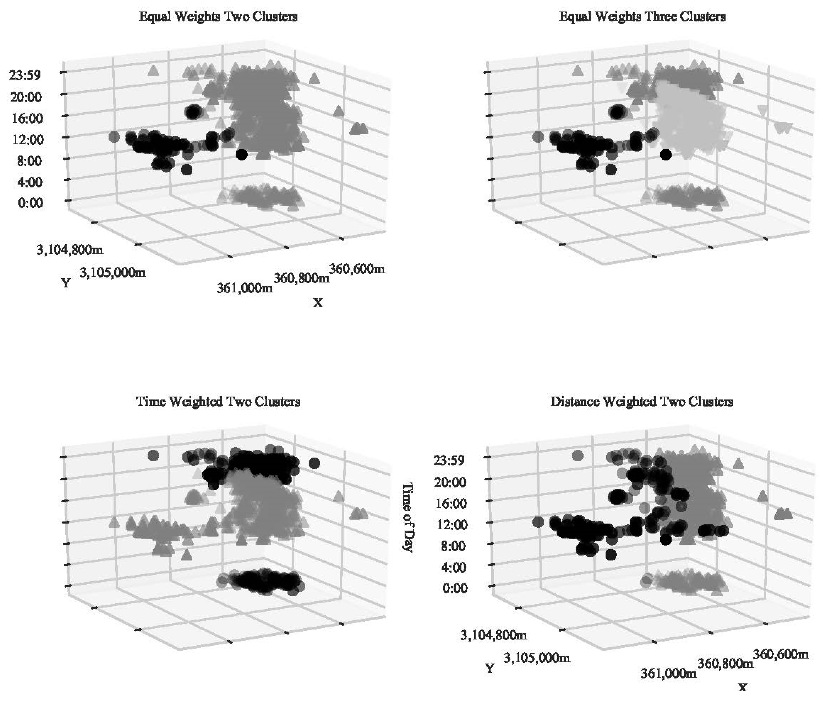
To demonstrate its application in practice, space–time hierarchical clustering was used to identify movement patterns in animal tracking data. The goal of the analysis was to identify any clusters, or hotspots, of activity within the animal’s home range, in both space and time [35,53,54]. For this example, a GPS data set for a Muscovy duck (Cairina mocahata) collected by Downs et al. [53] was used. Muscovy ducks are a nuisance species located in Florida, and native to Central and South America. They tend to have very infrequent flight patterns. The GPS data was collected from a single duck. The GPS device was set to record every four minutes, on for 15 h a day (beginning 05:39 in the morning), and off for nine hours at night (1003 observations). Figure 1 shows the distribution of the points with the DT. The period when the GPS device was turned off can be seen in a gap in the 3-dimensional views shown in Figure 6. For the space–time hierarchical clustering, the natural log of the sample size (number of observations) was used to determine the number of nearest neighbors (7 nearest neighbors), and 3600 s was used as the temporal scale factor.
The average silhouette score suggested that two or three clusters fit the data well. This is not surprising as there was visual evidence in Figure 1 of at least two different areas of activity in the west and east. Figure 6 presents an angle from viewing from the north to the south (to best show the temporal information). The two clusters in the upper left panel show the two areas that could be seen from Figure 1. The smaller section was most active around midday, whereas the larger section was active throughout the day. When 3 clusters are considered in the upper right panel, again the smaller section is separate, but now there are clusters showing activity late at night and midday in the larger area. This separation is useful in identifying activity centers at specific times of day.
Two further approaches to the space–time hierarchical clustering were considered with the Muscovy duck dataset. In the lower left panel, the distance component was given a low weight (0.2) and the temporal component a higher weight (1.0), emphasizing time over space. Here, the separation becomes between the activity around midday to late afternoon versus the activity late at night. Finally, in the lower-right corner the weights were reversed, emphasizing space over time. Here, the clusters show those two highly visited areas, but they are spread out over different parts of the day.
4. Discussion
This paper proposed an extension to the traditional hierarchical clustering method to incorporate space, time and attribute information. The space–time hierarchical clustering methodology is a flexible approach that can be applied to discrete time-stamped observation. While the approach is useful to any observation with a temporal component, particular emphasis was given to repeated observations, allowing clustering for data on a cycle. Also, the method focused on observations that were network constrained, or would benefit from a neighborhood structure appropriate for sequential data (e.g., the Delaunay triangulation). The proposed space–time hierarchical clustering approach is an improvement for this discrete time-event data, based on the comparisons to existing space-time clustering methods and the base hierarchical clustering approach. The distance metric is better able to handle the combined spatial and temporal distance, and the cyclical nature of the temporal data.
When compared to other clustering approaches, the method performed well against a ground-truth, particularly compared against a simple Euclidean based agglomerative approach. Overall, the ST-DBSCAN and space-time hierarchical clustering have different advantages. The ST-DBSCAN reduces noise and still performs relatively well on cyclical data. The space-time hierarchical clustering performs slightly better with cyclical data, and allows for different numbers of clusters to be evaluated and compared, but does not remove the noise in the data.
When applied to real data, the method was able to identify two main home ranges for the Muscovy Duck. It also made it possible to use the nested hierarchical structure to disaggregate the data into more clusters, and examine home ranges at different times. The weighting available in Equation (2) makes it possible to emphasize the different components depending on need. However, the data likely contained some potential GPS errors, and this noisy data was captured by the different clusters. Therefore, the physical area of the duck’s home range would likely be overestimated.
One of the known limitations of the agglomerative averaging approach to hierarchical clustering, is the algorithm will make a merging decision based on a static model (see Equation (1)). This may cause incorrect merging, especially when there is noise present in the data [55]. Many of the spatiotemporal clustering algorithms discussed above (ST-DBSCAN, ST-OPTICS, SNN-4D+) include an approach to remove or reduce noise in the clustering approach. To remove noise requires a clear definition of what noise is. Noise could be considered for each dimension separately, or as a whole. For spatial data, noise may come from errors in the GPS recording of the information, but this depends on the type and quantity of data. The space-time hierarchical clustering approach could be adapted to filter noise as part of a preprocess then proceed to the clustering.
Andrienko and Andrienko [29] suggest another potential limitation with the use of a weighted linear combination of the different components. They note that this combination can make the clusters difficult to interpret. At least, the distance results can be difficult to interpret since there are several pieces that make up the result. However, the use of a centrality measure or some performance metric might be used to identify important clusters, and can aid in the interpretation of the results. Also, knowing the original values associated with each observation in a cluster can help interpret them through descriptive statistics of the different variables.
Finally, performance may be a concern for working with large point datasets. The method adopted here was to produce a distance matrix that fed into hierarchical clustering algorithms. Depending on the programming language, this matrix may need to be held in memory (20,000 points produces a 20,000 × 20,000 size matrix). The solution adopted here to speed up the calculation and store less memory was to use sparse matrices (the dataset simulated above with 10,000 points took two minutes of processing time on a 6-core-processor with 16 gb of RAM). The approach would need to be adapted in different ways to handle datasets involving millions or billions of points.
Further work is needed to understand the weighting criteria, and how attribute information would affect the clustering using more real data. Also, adapting the method to potentially remove noise prior to developing the clusters may be a useful option when appropriate.
Author Contributions
Conceptualization, David S. Lamb and Joni Downs; Methodology, David S. Lamb; Validation, Steven Reader, and Joni Downs; Formal Analysis, David S. Lamb; Writing-Review & Editing, David S. Lamb, Joni Downs, and Steven Reader; Visualization, David S. Lamb; Supervision, Joni Downs and Steven Reader. All authors have read and agree to the published version of the manuscript.
Funding
This research received no external funding.
Conflicts of Interest
The authors declare no conflict of interest.
References
- Miller, H.J.; Han, J. (Eds.) Geographic Data Mining and Knowledge Discovery, 2nd ed.; CRC Press: Boca Raton, FL, USA, 2009; ISBN 978-1-4200-7397-3. [Google Scholar]
- Everitt, B.S.; Landau, S.; Leese, M.; Stahl, D. Hierarchical Clustering. In Cluster Analysis; John Wiley & Sons, Ltd.: Hoboken, NJ, USA, 2011; pp. 71–110. ISBN 978-0-470-97781-1. [Google Scholar]
- Han, J.; Lee, J.-G.; Kamber, M. An overview of clustering methods in geographic data analysis. In Geographic Data Mining and Knowledge Discovery; Miller, H.J., Han, J., Eds.; Taylor and Francis: Abingdon, UK, 2009; pp. 149–187. [Google Scholar]
- Yamada, I.; Rogerson, P.A. An Empirical Comparison of Edge Effect Correction Methods Applied to K-function Analysis. Geogr. Anal. 2003, 35, 97–109. [Google Scholar]
- Mennis, J.; Guo, D. Spatial data mining and geographic knowledge discovery—An introduction. Comput. Environ. Urban Syst. 2009, 33, 403–408. [Google Scholar] [CrossRef]
- Zhang, T.; Wang, J.; Cui, C.; Li, Y.; He, W.; Lu, Y.; Qiao, Q. Integrating Geovisual Analytics with Machine Learning for Human Mobility Pattern Discovery. ISPRS Int. J. Geo-Inf. 2019, 8, 434. [Google Scholar] [CrossRef] [Green Version]
- Long, J.A. Modeling movement probabilities within heterogeneous spatial fields. J. Spat. Inf. Sci. 2018, 16, 85–116. [Google Scholar] [CrossRef]
- Miller, H.J. A Measurement Theory for Time Geography. Geogr. Anal. 2005, 37, 17–45. [Google Scholar] [CrossRef]
- Miller, H.J. Modelling accessibility using space-time prism concepts within geographical information systems. Int. J. Geogr. Inf. Syst. 1991, 5, 287–301. [Google Scholar] [CrossRef]
- Richter, K.-F.; Schmid, F.; Laube, P. Semantic trajectory compression: Representing urban movement in a nutshell. J. Spat. Inf. Sci. 2012, 3–30. [Google Scholar] [CrossRef]
- Okabe, A.; Yamada, I. The K-Function Method on a Network and Its Computational Implementation. Geogr. Anal. 2001, 33, 271–290. [Google Scholar] [CrossRef]
- Yamada, I.; Thill, J.-C. Comparison of planar and network K-functions in traffic accident analysis. J. Transp. Geogr. 2004, 12, 149–158. [Google Scholar] [CrossRef]
- Okabe, A.; Sugihara, K. Spatial Analysis Along Networks: Statistical and Computational Methods; John Wiley & Sons: Hoboken, NJ, USA, 2012; ISBN 978-1-119-96776-7. [Google Scholar]
- Lamb, D.S.; Downs, J.A.; Lee, C. The network K-function in context: Examining the effects of network structure on the network K-function. Trans. GIS. 2015, 20, 448–460. [Google Scholar] [CrossRef]
- Manson, S.M. Does scale exist? An epistemological scale continuum for complex human–environment systems. Geoforum 2008, 39, 776–788. [Google Scholar] [CrossRef]
- Goodchild, M.F. Citizens as sensors: The world of volunteered geography. GeoJournal 2007, 69, 211–221. [Google Scholar] [CrossRef] [Green Version]
- Richardson, D.B. Real-Time Space–Time Integration in GIScience and Geography. Ann. Assoc. Am. Geogr. 2013, 103, 1062–1071. [Google Scholar] [CrossRef] [PubMed]
- Miller, H.J.; Goodchild, M.F. Data-driven geography. GeoJournal 2015, 80, 449–461. [Google Scholar] [CrossRef]
- Miller, H.J. Activity-Based Analysis. In Handbook of Regional Science; Fischer, M.M., Nijkamp, P., Eds.; Springer: Berlin/Heidelberg, Germany, 2014; pp. 705–724. ISBN 978-3-642-23429-3. [Google Scholar]
- Ashbrook, D.; Starner, T. Using GPS to Learn Significant Locations and Predict Movement Across Multiple Users. Pers. Ubiquitous Comput 2003, 7, 275–286. [Google Scholar] [CrossRef]
- Andrienko, G.; Andrienko, N.; Bak, P.; Keim, D.; Wrobel, S. Visual Analytics of Movement; Springer: Berlin/Heidelberg, Germany, 2013; ISBN 978-3-642-37582-8. [Google Scholar]
- Birant, D.; Kut, A. ST-DBSCAN: An algorithm for clustering spatial–temporal data. Data Knowl. Eng. 2007, 60, 208–221. [Google Scholar] [CrossRef]
- Everitt, B.S.; Landau, S.; Leese, M.; Stahl, D. An Introduction to Classification and Clustering. In Cluster Analysis; John Wiley & Sons, Ltd.: Hoboken, NJ, USA, 2011; pp. 1–13. ISBN 978-0-470-97781-1. [Google Scholar]
- Guo, D. Multivariate Spatial Clustering and Geovisualization. In Geographic Data Mining and Knowledge Discovery; Miller, H., Han, J., Eds.; CRC Press: Boca Raton, FL, USA, 2009; pp. 325–345. [Google Scholar]
- Kisilevich, S.; Mansmann, F.; Nanni, M.; Rinzivillo, S. Spatio-temporal clustering. In Data Mining and Knowledge Discovery Handbook; Maimon, O., Rokach, L., Eds.; Springer: Berlin/Heidelberg, Germany, 2009; pp. 855–874. ISBN 978-0-387-09822-7. [Google Scholar]
- Wang, M.; Wang, A.; Li, A. Mining Spatial-temporal Clusters from Geo-databases. In Proceedings of the Advanced Data Mining and Applications: Second International Conference, ADMA 2006, Xi’an, China, 14–16 August 2006. [Google Scholar]
- Agrawal, K.P.; Garg, S.; Sharma, S.; Patel, P. Development and validation of OPTICS based spatio-temporal clustering technique. Inf. Sci. 2016, 369, 388–401. [Google Scholar] [CrossRef]
- Wardlaw, R.L.; Frohlich, C.; Davis, S.D. Evaluation of precursory seismic quiescence in sixteen subduction zones using single-link cluster analysis. Pure Appl. Geophys. 1990, 134, 57–78. [Google Scholar] [CrossRef]
- Andrienko, G.; Andrienko, N. Interactive Cluster Analysis of Diverse Types of Spatiotemporal Data. SIGKDD Explor Newsl 2010, 11, 19–28. [Google Scholar] [CrossRef]
- Oliveira, R.; Santos, M.Y.; Moura Pires, J. 4D+SNN: A Spatio-Temporal Density-Based Clustering Approach with 4D Similarity. In Proceedings of the 2013 IEEE 13th International Conference on Data Mining Workshops (ICDMW), Dallas, TX, USA, 7–10 December 2013; pp. 1045–1052. [Google Scholar]
- Bermingham, L.; Lee, I. A framework of spatio-temporal trajectory simplification methods. Int. J. Geogr. Inf. Sci. 2017, 31, 1128–1153. [Google Scholar] [CrossRef]
- Lee, J.-G.; Han, J.; Whang, K.-Y. Trajectory clustering: A partition-and-group framework. In Proceedings of the 2007 ACM SIGMOD International Conference on Management of Data, Beijing, China, 11–14 June 2007; pp. 593–604. [Google Scholar]
- Guo, N.; Shekhar, S.; Xiong, W.; Chen, L.; Jing, N. UTSM: A Trajectory Similarity Measure Considering Uncertainty Based on an Amended Ellipse Model. ISPRS Int. J. Geo-Inf. 2019, 8, 518. [Google Scholar] [CrossRef] [Green Version]
- Sokal, R.R.; Michener, C.D. A statistical method for evaluating systematic relationships. Univ. Kans. Sci. Bull. 1958, 38, 1409–1438. [Google Scholar]
- Downs, J.A.; Horner, M.W. Analysing infrequently sampled animal tracking data by incorporating generalized movement trajectories with kernel density estimation. Comput. Environ. Urban Syst. 2012, 36, 302–310. [Google Scholar] [CrossRef]
- McGuire, M.P.; Janeja, V.; Gangopadhyay, A. Mining sensor datasets with spatiotemporal neighborhoods. J. Spat. Inf. Sci. 2013. [Google Scholar] [CrossRef]
- Okabe, A.; Boots, B.; Sugihara, K.; Chiu, S.N. Spatial Tessellations: Concepts and Applications of Voronoi Diagrams; John Wiley & Sons: Hoboken, NJ, USA, 2009; ISBN 978-0-470-31785-3. [Google Scholar]
- Gibbons, A. Algorithmic Graph Theory; Cambridge University Press: New York, NY, USA, 1985; ISBN 9780521288811. [Google Scholar]
- Di Pierro, M. Annotated Algorithms in Python with Applications in Physics, Biology, and Finance; EXPERTS4SOLUTIONS: Chicago, IL, USA, 2013; ISBN 978-0-9911604-0-2. [Google Scholar]
- Huang, B.; Wu, Q.; Zhan, F.B. A shortest path algorithm with novel heuristics for dynamic transportation networks. Int. J. Geogr. Inf. Sci. 2007, 21, 625–644. [Google Scholar] [CrossRef]
- Ertoz, L.; Steinbach, M.; Kumar, V. A new shared nearest neighbor clustering algorithm and its applications. In Proceedings of the Workshop on Clustering High Dimensional Data and its Applications at 2nd SIAM International Conference on Data Mining, Arlington, VA, USA, 11–13 April 2002; pp. 105–115. [Google Scholar]
- Oliphant, T.E. Python for Scientific Computing. Comput. Sci. & Eng. 2007, 9, 10–20. [Google Scholar]
- Hagberg, A.A.; Schult, D.A.; Swart, P.J. Exploring network structure, dynamics, and function using NetworkX. In Proceedings of the 7th Python in Science Conference (SciPy2008), Pasadena, CA USA, 19–24 August 2008; pp. 11–15. [Google Scholar]
- McMaster, R.B.; Sheppard, E. Introduction: Scale and Geographic Inquiry. In Scale and Geographic Inquiry; Sheppard, E., McMaster, R.B., Eds.; Blackwell Publishing Ltd.: Malden, MA, USA, 2004; pp. 1–22. ISBN 978-0-470-99914-1. [Google Scholar]
- Levin, S.A. The Problem of Pattern and Scale in Ecology: The Robert H. MacArthur Award Lecture. Ecology 1992, 73, 1943–1967. [Google Scholar] [CrossRef]
- Fotheringham, A.S.; Wong, D.W.S. The Modifiable Areal Unit Problem in Multivariate Statistical Analysis. Environ. Plan. A 1991, 23, 1025–1044. [Google Scholar] [CrossRef]
- Kwan, M.-P. The Uncertain Geographic Context Problem. Ann. Assoc. Am. Geogr. 2012, 102, 958–968. [Google Scholar] [CrossRef]
- Kwan, M.-P. Algorithmic Geographies: Big Data, Algorithmic Uncertainty, and the Production of Geographic Knowledge. Ann. Am. Assoc. Geogr. 2016, 106, 274–282. [Google Scholar]
- Pedregosa, F.; Varoquaux, G.; Gramfort, A.; Michel, V.; Thirion, B.; Grisel, O.; Blondel, M.; Prettenhofer, P.; Weiss, R.; Dubourg, V.; et al. Scikit-learn: Machine Learning in Python. J. Mach. Learn. Res. 2011, 12, 2825–2830. [Google Scholar]
- Hubert, L.; Arabie, P. Comparing partitions. J. Classif. 1985, 2, 193–218. [Google Scholar] [CrossRef]
- Rosenberg, A.; Hirschberg, J. V-Measure: A Conditional Entropy-Based External Cluster Evaluation Measure. In Proceedings of the EMNLP-CoNLL, Prague, Czech Republic, 28–30 June 2007; Volume 7, pp. 410–420. [Google Scholar]
- Pavlis, M.; Dolega, L.; Singleton, A. A Modified DBSCAN Clustering Method to Estimate Retail Center Extent. Geogr. Anal. 2017. [Google Scholar] [CrossRef]
- Downs, J.A.; Horner, M.W.; Hyzer, G.; Lamb, D.; Loraamm, R. Voxel-based probabilistic space-time prisms for analysing animal movements and habitat use. Int. J. Geogr. Inf. Sci. 2014, 28, 875–890. [Google Scholar] [CrossRef]
- Gao, P.; Kupfer, J.A.; Zhu, X.; Guo, D. Quantifying Animal Trajectories Using Spatial Aggregation and Sequence Analysis: A Case Study of Differentiating Trajectories of Multiple Species. Geogr. Anal. 2016, 48, 275–291. [Google Scholar] [CrossRef]
- Karypis, G.; Han, E.-H.; Kumar, V. Chameleon: Hierarchical clustering using dynamic modeling. Computer 1999, 32, 68–75. [Google Scholar] [CrossRef] [Green Version]
Figure 1.
Example of a Delaunay Triangulation using animal tracking points.

Figure 2.
Considerations for the time component. Top panel presents temporal distance from 12 h (midday), and the bottom panel presents distance from midnight.
Figure 2.
Considerations for the time component. Top panel presents temporal distance from 12 h (midday), and the bottom panel presents distance from midnight.

Figure 3.
Example simulated datasets of random different cluster groupings, used to evaluate the nearest neighbor and temporal scale parameters.
Figure 3.
Example simulated datasets of random different cluster groupings, used to evaluate the nearest neighbor and temporal scale parameters.

Figure 4.
Average scores across different values for nearest neighbors across all the temporal scale values (A), and for different values of the temporal scale across all nearest neighbor scale values (B).
Figure 4.
Average scores across different values for nearest neighbors across all the temporal scale values (A), and for different values of the temporal scale across all nearest neighbor scale values (B).

Figure 5.
Simulated dataset that is used for comparing different clustering approaches.

Figure 6.
Applied Space-Time Hierarchical Clustering to clustering of GPS observations of a Muscovy Duck.
Figure 6.
Applied Space-Time Hierarchical Clustering to clustering of GPS observations of a Muscovy Duck.


Table 1.
Summary of clustering classifications and the common algorithms used to achieve partitioning, hierarchical, density-based, or grid-based approaches [3,23].
| Clustering Classification | Description | Common Algorithms |
|---|---|---|
| Partitioning | Partitions the data into a user specified number of groups. Each point belongs to one group. Does not work well for irregularly shaped clusters. | k-means, k-medoids, clustering large applications based randomized search (CLARANS), and Expectation-Maximization (EM) algorithm. |
| Hierarchical | Decomposes data into a hierarchy of groups, each larger group contains a set of subgroups. Two methods: agglomerative (builds groups from the observation up), or divisive (start with a large group and separate). | Balanced iterative reducing and clustering using hierarchies (BIRCH), Chameleon, Ward’s Method, Nearest Neighbor, (Dendrograms are used to visualize the hierarchy). |
| Density-based | Useful for irregularly shaped clusters. Clusters grow based on a threshold for the number of objects in a neighborhood. | DBSCAN, ordering points to identify cluster structure (OPTICS) and density based clustering (DENCLUE), SNN |
| Grid-based | Region is divided in to a grid of cells, and clustering is performed on the grid structure. | statistical information grid (STING), WaveCluster, and clustering in quest (CLIQUE) |
Table 2.
Comparison of the different clustering algorithm and the performance compared to the true clusters.
Table 2.
Comparison of the different clustering algorithm and the performance compared to the true clusters.
| Method and Parameters | Clusters Selected or Identified | Homogeneity Score | Adjusted Random Index |
|---|---|---|---|
| Hierarchical Clustering with Euclidean Distance and average linkage | 20 | 0.79 | 0.59 |
| Space-Time Hierarchical clustering (Nearest Neighbors = 7, time scale = 3600) | 20 | 0.89 | 0.77 |
| Space-Time Hierarchical clustering (Nearest Neighbors = 7, time scale = 3600) | 15 | 0.83 | 0.65 |
| ST-DBSCAN (Spatial Threshold = 5000, Temporal Threshold = 3600, MinPts = 7 | 15 + Noise | 0.75 | 0.52 |
| ST-DBSCAN (Spatial Threshold = 8000, Temporal Threshold = 1800, MinPts = 1) | 20 + Noise | 0.85 | 0.66 |
| ST-DBSCAN (Spatial Threshold = 5000, Temporal Threshold = 3600, MinPts = 2) | 20 + Noise | 0.82 | 0.62 |
| DBSCAN (eps = 0.05, Minimum Samples = 2) | 20 + Noise | 0.85 | 0.67 |
© 2020 by the authors. Licensee MDPI, Basel, Switzerland. This article is an open access article distributed under the terms and conditions of the Creative Commons Attribution (CC BY) license (http://creativecommons.org/licenses/by/4.0/).
Share and Cite
MDPI and ACS Style
Lamb, D.S.; Downs, J.; Reader, S. Space-Time Hierarchical Clustering for Identifying Clusters in Spatiotemporal Point Data. ISPRS Int. J. Geo-Inf. 2020, 9, 85. https://0-doi-org.brum.beds.ac.uk/10.3390/ijgi9020085
AMA Style
Lamb DS, Downs J, Reader S. Space-Time Hierarchical Clustering for Identifying Clusters in Spatiotemporal Point Data. ISPRS International Journal of Geo-Information. 2020; 9(2):85. https://0-doi-org.brum.beds.ac.uk/10.3390/ijgi9020085
Chicago/Turabian StyleLamb, David S., Joni Downs, and Steven Reader. 2020. "Space-Time Hierarchical Clustering for Identifying Clusters in Spatiotemporal Point Data" ISPRS International Journal of Geo-Information 9, no. 2: 85. https://0-doi-org.brum.beds.ac.uk/10.3390/ijgi9020085
Note that from the first issue of 2016, this journal uses article numbers instead of page numbers. See further details here.