Numerical Simulation of Donghu Lake Hydrodynamics and Water Quality Based on Remote Sensing and MIKE 21

1
School of Hydropower Engineering & Information Engineering, Huazhong University of Science & Technology, Wuhan 430074, China
2
Shanghai Academy of Spaceflight Technology, Shanghai 200000, China
*
Author to whom correspondence should be addressed.
ISPRS Int. J. Geo-Inf. 2020, 9(2), 94; https://0-doi-org.brum.beds.ac.uk/10.3390/ijgi9020094
Submission received: 3 December 2019
/
Revised: 20 January 2020
/
Accepted: 27 January 2020
/
Published: 4 February 2020
Abstract
:Numerical simulation is an important method used in studying the evolution mechanisms of lake water quality. At the same time, lake water quality inversion technology using the characteristics of spatial optical continuity data from remote sensing satellites is constantly improving. It is, however, a research hotspot to combine the spatial and temporal advantages of both methods, in order to develop accurate simulation and prediction technology for lake water quality. This paper takes Donghu Lake in Wuhan as its research area. The spatial data from remote sensing and water quality monitoring information was used to construct a multi-source nonlinear regression fitting model (genetic algorithm (GA)-back propagation (BP) model) to invert the water quality of the lake. Based on the meteorological and hydrological data, as well as basic water quality data, a hydrodynamic model was established by using the MIKE21 model to simulate the evolution rules of water quality in Donghu Lake. Combining the advantages of the two, the best inversion results were used to provide a data supplement for optimization of the water quality simulation process, improving the accuracy and quality of the simulation. The statistical results were compared with water quality simulation results based on the data measured. The results show that the water quality simulation of chlorophyll a and nitrate nitrogen mean square errors fell to 17% and 24%, from 19% and 31% respectively, after optimization using remote sensing spatial information. The model precision was thus improved, and this is consistent with the actual pollution situation of Donghu Lake.
1. Introduction
The water quality issue has become serious, due to increasing eutrophication in shallow lakes [1]. About three-quarters of urban lakes in China are affected by eutrophication at present, which has become one of the main problems in their management [2].
Numerical simulation of the water environment is a process of expressing the basic water information and its spatio-temporal variation in mathematical language. It includes both hydrodynamic and water quality numerical simulation [3]. Research on the subject began in 1925, more than 90 years before it was fully developed. It was introduced into mainland China in the 1970s, and has been widely applied in various fields since then, becoming an important means of studying inland water and associated environmental problems [4]. Numerical simulation of water quality can be used to explore its evolution and predict how it will change in the future under specific conditions. The simulation results can be applied to the evaluation of inland lake eutrophication and water quality index monitoring, which has become an important component of lake water environmental studies [5].
Common models that can combine hydrodynamic processes with biochemical water quality changes include Delft3D, Water Quality Analysis Simulation Program (WASP), the environmental fluid dynamics code (EFDC), MIKE, and so on. Liu et al. [6] took the Songhua River in northeast China as their research area, analyzed the permissible pollution situation in the basin using the MIKE model, and proposed reasoned, scientific improvement measures. Wang et al. [7] applied the WASP model to the prediction and evaluation of the water environment in the Harbin section of Songhua river basin, and obtained a good simulation. Liu et al. [8] carried out the whole EFDC model packaging and integration research process, and realized the business operation with low modification and high efficiency. WASP can be applied to the simulation of quality in various types of water, but it is inferior to EFDC in three-dimensional hydrodynamic simulations. Although the EFDC model source code was made public, and can be freely accessed, the encapsulated business model is expensive, requiring a long period of in-depth study, with a large amount of difficult data acquisition. The MIKE series models include hydrological process simulation and prediction of the water environment and basin characteristics. MIKE has a well-designed interactive interface operation, and can integrate seamlessly with geographical information systems (GISs), AutoCAD, and other engineering applications. After a long period of practical application in China, it has been widely approved and applied.
The process of water quality numerical simulation has a high demand for measurement data, in contrast to the quantity required for conventional water quality monitoring, which is limited as it relies only on manual sampling of selected points. For this reason, it is difficult to obtain continuously distributed water quality monitoring results in space and time [9].
Remote sensing of water quality is a new monitoring method which can measure optical water information periodically over a large area, and has been widely used at home and abroad [10]. It can quickly and accurately obtain a continuous spatial data distribution of water quality monitoring indexes [11], and overcomes the difficulties associated with obtaining small amounts of physically measured data.
There are many inland water quality indicators that can be monitored by remote sensing, including all aspects of the physics, biology and chemistry. They can be divided into two types: color-based parameters (such as chlorophyll, suspended solids etc.) and non-color-based parameters (total phosphorus, total nitrogen etc.), among which most of the inversion studies have been on chlorophyll a, total nitrogen and total phosphorus [12].
There are four main methods of chlorophyll remote sensing inversion: empirical, semi-empirical, analytical, and physical. Yunfang Z et al. [13] established a traditional BP-ANN model for Lake Taihu in Jiangsu province based on multi-spectral remote sensing from a multi-source satellite and real-time water quality data measured on the ground. This was used to simulate the nonlinear regression relationship between the spectrum and the concentrations of water quality index parameters. Shi Rui et al. [14] constructed a chlorophyll a inversion model by combining wavelet analysis with a neural network model, based on Landsat thematic TM image data and the chlorophyll a data collected from an environmental monitoring station. The research was carried out at Wuliangsuhai Lake in Inner Mongolia and provided satisfactory results, helping to improve water quality detection technology at the lake. Domestic scholars have also done a lot of related research. Cao et al. [15], working at Weishan Lake, built a variety of empirical and collection models to apply water quality inversion using hyperspectral multiphase data, the measured chlorophyll a, total suspended solids and turbidity data. This proved that the particle swarm optimization algorithm combined with the support vector machine collection model produces the most accurate simulations.
Some scholars at home and abroad make full use of the remote sensing spectral information combined heuristic intelligent algorithm to establish nonlinear multi-source regression fitting model for non-aqueous index (such as total nitrogen (TN), total phosphorus (TP), etc.) inversion analysis. Wang et al. [16] established an artificial neural network algorithm model based on TM remote sensing images and TP, TN data, and conducted nutrient concentration inversion analysis in the study area of Poyang Lake. Chang et al. [17] studied and analyzed the spatial state distribution of total phosphorus in Tampa bay, Florida, USA by using the heuristic intelligent genetic algorithm theory and based on MODIS satellite images to establish a complex nonlinear regression model. Some domestic scholars also established the correlation between total nitrogen and total phosphorus and sensitive band values by analyzing the spectral characteristics of total nitrogen and total phosphorus, so as to achieve quantitative inversion.
However, remote sensing can only collect instantaneous information from the water surface. It is unable to predict the dynamic evolution of a water body over time.
In conclusion, the two methods are now optimized for lake water quality studies and complement each other. The mature numerical model of the hydrological environment is combined with the still-developing remote sensing inversion technology. It can not only follow evolution mechanisms, but can also improve the numerical simulations, finally producing accurate water quality results. This is now the first choice for lake eutrophication management in a new environment [18]. At present, there are only a few applications in water quality monitoring and pollution control of shallow lakes in China, which has important exploration and research significance.
In this paper, we have carried out a water quality inversion of Donghu Lake in Wuhan, combining it with an empirical quantitative inversion model using measured water quality data and synchronous remote sensing image data from the lake monitoring points. Based on MIKE21, a numerical coupling model was established, using the meteorological and hydrological data, and the water quality of Donghu Lake was simulated. In addition, remote sensing inversion and water quality numerical simulation are combined; that is, the best inversion results are selected as the initial and boundary conditions of the water quality numerical model to supplement and optimize the data in the simulation process. Finally, the results of the optimization and traditional simulation are compared and analyzed.
2. Study Area
Located to the south of the Yangtze River in Wuhan Hubei Province (30°33′33.0″ N, 114°24′38.5″ E), Lake Donghu is one of the largest urban lakes in China, having both abundant rainfall and sunshine [19]. The dimensions of the Donghu Lake are as follows: the basin area is 187 km2, the lake surface area is 34.27 km2; the lake length is 11.3 km; the largest lake width is 10.3 km; the shoreline length is 121.7 km; the maximum water depth is 4.75 m; the average water depth is 2.21 m, and the total volume of the lake is about 6.2 million m3.
Since the end of the last century, Donghu Lake has been divided into several sub-lakes by artificial intervention. It is composed of Xiaotan and Tangling lakes in the north; Shaohji, Fruit, Miao and Guozheng lakes in the southwest; and Tuanhu, Yujia and Hou lakes in the southeast. The regional environments and connectivity of the water systems between the different sub-lakes are different. There are port channels around the lake. It is connected with the Yangtze River system through the Qingshan port gate, the Zengjiaxiang pumping station and the Luojia road gate, forming a diversion and drainage loop.
After the 1980s, with the growth of urban economic construction, many areas of Donghu Lake have silted up, and the connections with the surrounding lakes have been affected by human interference. The original channel of the port was severely reduced in size and disappeared. The water flow from the Yangtze River was also affected, resulting in a low frequency and degree of water exchange. The water quality is gradually deteriorating, and aquatic biodiversity is also decreasing. Most of the water quality categories are class IV and class V, and some of them are even lower. Since 1983, there has been implementation of the Donghu Lake comprehensive treatment project, which mainly focuses on sewage interception and sewage purification. The results of water quality monitoring in Hubei Province by the Hubei Provincial Environmental Protection Department from 2013 to 2017 show that Donghu Lake basically maintained a stable class IV water quality, and an average status between mild and moderate eutrophication. Chemical oxygen demand and total phosphorus are the main indicators of over class III. In recent years, the eutrophication of Donghu Lake has become severe, and algal blooms of different degrees have appeared. It is, therefore, urgent to improve the monitoring of lake eutrophication and to improve the water quality of Donghu Lake.
3. Research Methodology
3.1. MIKE21 Model
MIKE21 software is produced by DHI (previously Danish Institute for Water and Environment). It has undergone decades of development, and has been continuously improved. MIKE21 software has a powerful processing capability in the spatiotemporal numerical simulation of free surface flow of shallow water. It is widely applied to large projects in China, and was used in this study to simulate the hydrodynamic and water quality evolution of Donghu Lake.
3.1.1. Hydrodynamic Module
MIKE21 Flow Mode FM was adopted to simulate the hydrodynamic environment of Donghu Lake waters, including the hydrodynamic model (HD) and the hydrodynamic advection diffusion model (AD).
The hydrodynamic model (HD) simulates the changes of water level and water flow with time due to various forces. The model is based on Navies-Stokes equations with three-dimensional incompressibility and uniform distributions of Reynolds values. It is subject to the Boussinesq assumption and the hydrostatic pressure assumption.
There are various meteorological conditions, such as wind, and a wide range of free water flows on the surface of the Donghu Lake. The vertical direction is mainly shallow water with low velocity. The vertical acceleration is much less than gravitational acceleration, and the vertical turbulence effect is relatively small. The hydrostatic pressure assumption and the Boussinesq eddy viscosity assumption are, therefore, satisfied. The governing equation, that is, the basic motion equation of two-dimensional unsteady water flow, is as follows:
Continuity equation:
Momentum equation:
In the X direction:
In the Y direction:
where x, y and z are right-handed Cartesian coordinates; t is time; h is the total water depth (h = d + η, where d is the resting depth, and η is the water level elevation); is the density of (fresh) water; u, v and w are the velocity components in the x, y, and z directions; g is the acceleration due to gravity; f (the Coriolis force coefficient) = 2Ω sinφ and (Ω is angular velocity of rotation; φ is the geographic latitude); is the radiation stress tensor; S and (, ) are the discharge and discharge speed of the pollution point source respectively; and are the average values of the velocity at the vertical depth; and are lateral stress (including viscous friction, turbulent friction, differential convection friction); , and , A is the eddy viscosity coefficient of the horizontal flow.
The delimitation condition contains the initial and boundary conditions required to solve the above equation. The boundary conditions include the closed boundary, the open boundary, and the dry and wet boundary. Along the closed boundary (i.e., the land boundary), all variables flowing perpendicular to the boundary must be 0. Open boundary conditions can be specified as flow or water level processes. The dry and wet boundary unit is defined as dry, semi-dry and wet to determine the flooded boundary. Initial conditions include background values corresponding to the flow field, such as water level, flow, and flow velocity. First, the initial values corresponding to the model boundary should be set to obtain the initial values of each cell in the grid computing area, and then the hydrodynamic model should be run until the flow field is stable.
The hydrodynamic advection diffusion model (AD) is a water pollutant transport equation. When combined with the HD model, the convection, diffusion, and other transport processes of dissolved pollutants in water can be simulated. According to the law of conservation of mass, considering the factors of convective diffusion and degradation in pollutant migration processes, the migration equation can be solved:
where c is the concentration of pollutants; the linear attenuation coefficient; and is the x, y diffusion coefficient, respectively.
3.1.2. Water Quality Module
The water quality module (WQ) is used to describe the degradation of organic matter and the oxygen environment in water. The eutrophication module (EU) is used to describe nutrient circulation in water, the growth of phytoplankton and plants, as well as the growth and distribution of algae. The heavy metal module (ME) describes the adsorption and desorption processes between heavy metals and suspended solids in water and the metal exchange process between sediment particles and pore water.
3.2. Remote Sensing Inversion Model
In the back propagation (BP) neural network model, it is easy to fall into local extreme values during training. This study, therefore, uses a genetic algorithm (GA) to optimize the BP neural network model, in order to establish the GA-BP regression model for water quality inversion of Donghu Lake.
3.2.1. BP Neural Network Optimized by GA
In recent years, the BP artificial neural network has been widely used in the inversion of ocean water color for algal bloom research [20]. This is effective when simulating the complex relationship between remote sensing spectral characteristics and water color parameters without clearly understanding the internal mechanism. However, there are also limitations of the BP neural network. For example, the network training tends to fall into the saturation zone of the S-type function, leading to a local minimum value, so it is difficult to reach the minimum mean square error (MSE). In the process of network learning, the convergence speed is slow and the learning and memory are unstable. The influence of human input on the parameters will make the training results of the BP network vary greatly.
The genetic algorithm adopts a multi-solution parallel search for optimization, which can prevent premature convergence due to local optimization in network training.
3.2.2. Model Implementation
The GA optimized BP neural network consists of three parts: determination of topology structure of the BP neural network; optimization of the genetic algorithm and searching for parameters; and training and prediction of the BP neural network. The BP neural network topology is determined according to the number of input and output parameters in actual engineering problems, and then the length of individual sections (chromosomes) of the genetic algorithm is determined. The BP neural network parameters were initialized, and the weight and threshold were obtained after GA optimization. In this case, each chromosome in the population contained all weights and thresholds of the network. The fitness value of individuals is calculated by the fitness function, and the genetic algorithm finds the optimal fitness value of individuals by selecting, crossing, and mutating. The BP neural network uses the optimal individual to assign a value to the network weight threshold and train the network. The algorithm flow chart corresponding to the output prediction result is shown in Figure 1.
Based on the above theory, the GA was used to optimize the algorithm flow of the BP neural network using MATLAB programming, and the nonlinear regression fitting model was built. The genetic algorithm was used to seek the optimal weight threshold parameters, and the training process of the BP neural network was optimized to improve the accuracy of model output.
4. Hydrodynamic and Water Quality Numerical Simulation of Donghu Lake
4.1. Remote Sensing Inversion of Water Quality in Donghu Lake
Based on the improved back propagation neural network model of the genetic algorithm, this study established the relationship between the water quality index and the spectral reflectivity of the lake, to obtain the predicted value of the water quality index.
4.1.1. Data Sources and Data Processing
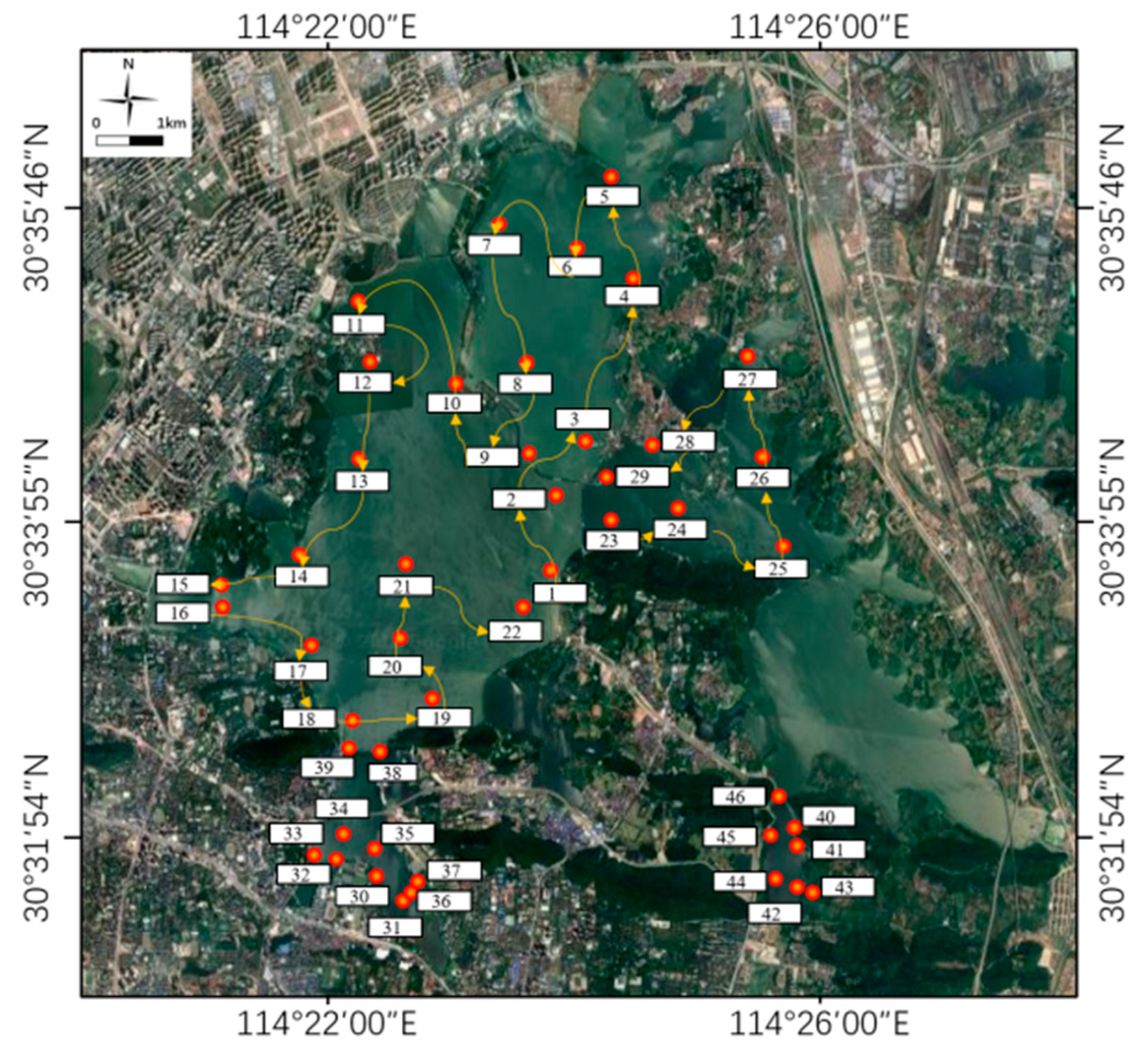
The data required for the study included both remote sensing and measured data. The measured data included total phosphorus (TP), total nitrogen (TN), chlorophyll a, chemical oxygen demand (COD), dissolved oxygen (DO), water temperature, pH, and turbidity. Data samples were collected for November 2017, December 2017, March 2018, and October 2018 (see Table 1 and Figure 2). There were 30 sampling sites in November 2017, 46 in December 2017, 48 in March 2008, and 43 in October 2008.
The measured data were obtained from the Simulation Center 201 of the School of Hydropower and Digital Engineering, Huazhong University of Science and Technology. According to the synchronization or quasi-synchronization principle of remote sensing inversion, students complete water quality measurement once a month according to the date of Landsat8 data. Students collected water samples from Donghu Lake and conducted chemical determination and water quality parameter analyses in the environmental laboratory, finally obtaining the measured water quality data from the Donghu Lake research area.
The remote sensing used Landsat-8 data with a spatial resolution of 30 m and a band range of 0.43–0.89 μm, b1–b5 respectively. Landsat-8 images corresponding to the actual water quality sampling time were used in order to ensure the spatio-temporal synchronization of images and measured data.
4.1.2. GA-BP Model Training
The GA-BP regression model was trained by using the measured water quality in November and December 2017 and the corresponding spectral processing data from Donghu Lake. The basic parameters of the optimization model are shown in Table 2.
4.1.3. GA-BP Model Validation
First, the water quality values were fed into the optimization model with the MATLAB tool. Then, the measured training data set was input to train the network model. Finally, the test data set was used for model verification and accuracy evaluation, and the statistical results were obtained (Figure 3).
Figure 3 shows the correlation coefficient statistical results of training, test, verification and the overall sample, the mean square error (MSE) trend of the model, the trend of fitness curve in the evolution of genetic algorithm and the contrast between expected value and the expected value during the simulation of chlorophyll a concentration in Donghu Lake.
The genetic algorithm was terminated in the 50th generation (see Figure 1). The error value decreased gradually, and the fitness value of the corresponding optimal individual was 2.47. Fitness is used to evaluate the quality of an individual, and the more fit the individual, the better. The model achieved the best fitting effect at the 15th iteration, and the corresponding minimum MSE was 0.055. The total correlation coefficient (R) of the model reached 0.869, and the simulation effect was good.
4.1.4. GA-BP Model Application
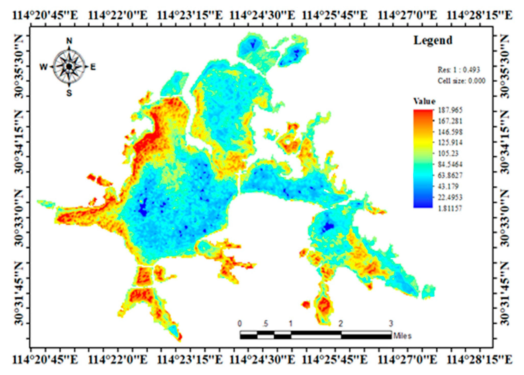
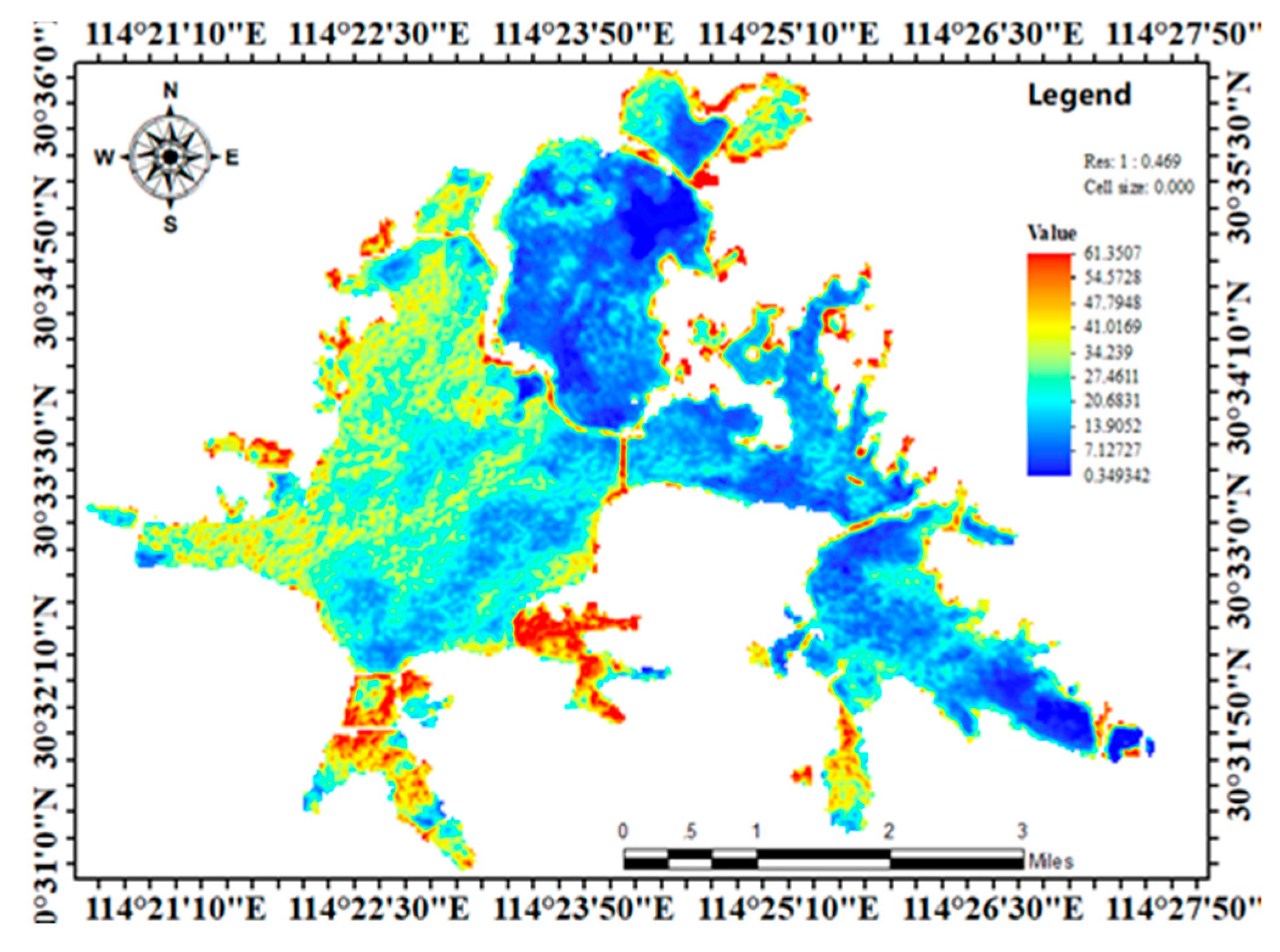
The chlorophyll a concentration of Donghu Lake was predicted based on the trained optimization inversion model using the remote sensing data set as the input data (15 November and 17 December). The kriging tool of ArcGIS was used to carry out interpolation. A thematic distribution map was made, and the results of the inversion distribution of chlorophyll a concentration in the Donghu Lake were can be seen in Figure 4 and Figure 5.
As shown in Figure 4, the chlorophyll a concentration of district closing to the periphery of the southwest bank of Donghu Lake in November 2017 was generally poor, which basically remained in class 4 and 5. The water quality gradually improved close to the central area of the lake and mainly remained in class 1 and 2. The overall distribution is consistent with the actual situation, which is consistent with the measured value obtained from the site, and the inversion result is good.
As shown in Figure 5, the inversion value distribution of chlorophyll a concentration in December also conforms to the actual situation in space and the actual measurement in local areas.
Moreover, compared with November, the average temperature in December falls. The algae grow more slowly, and the chlorophyll a content of the body of water should be decreased. It can be seen in the quantitative relation of two month inversion distribution that the simulation value of the model conforms to the actual situation. The results of the GA-BP neural network inversion model are proved to be reasonable and reliable in practice.
4.2. Hydrodynamics Numerical Simulation of Donghu Lake
The first step of hydrodynamic water quality simulation requires digital generalization of the actual water topography as the basis of modeling. In this study, a hydrodynamic model of Donghu Lake was established based on the MIKE21 FM module. The main stages are: (1) preparation of topographic and bathymetric data to determine the calculated area; (2) division of unstructured meshes using the mesh generator; (3) establishment of the time series file as the boundary condition of the model; (4) set up of the hydrodynamic file, the parameters, and saving of the running simulation; and (5) post-processing of results (parameter calibration and model validation).
4.2.1. Grid Division of Study Area
The Donghu Lake terrain was divided based on an unstructured mesh generator from MIKE ZERO. An unstructured mesh is a finite element mesh composed of any triangle or quadrilateral. The size, shape and node position of grid cells can be adjusted flexibly. Compared with a structured grid, it has greater adaptability to complex boundaries and can thus produce a better fit to the terrain.
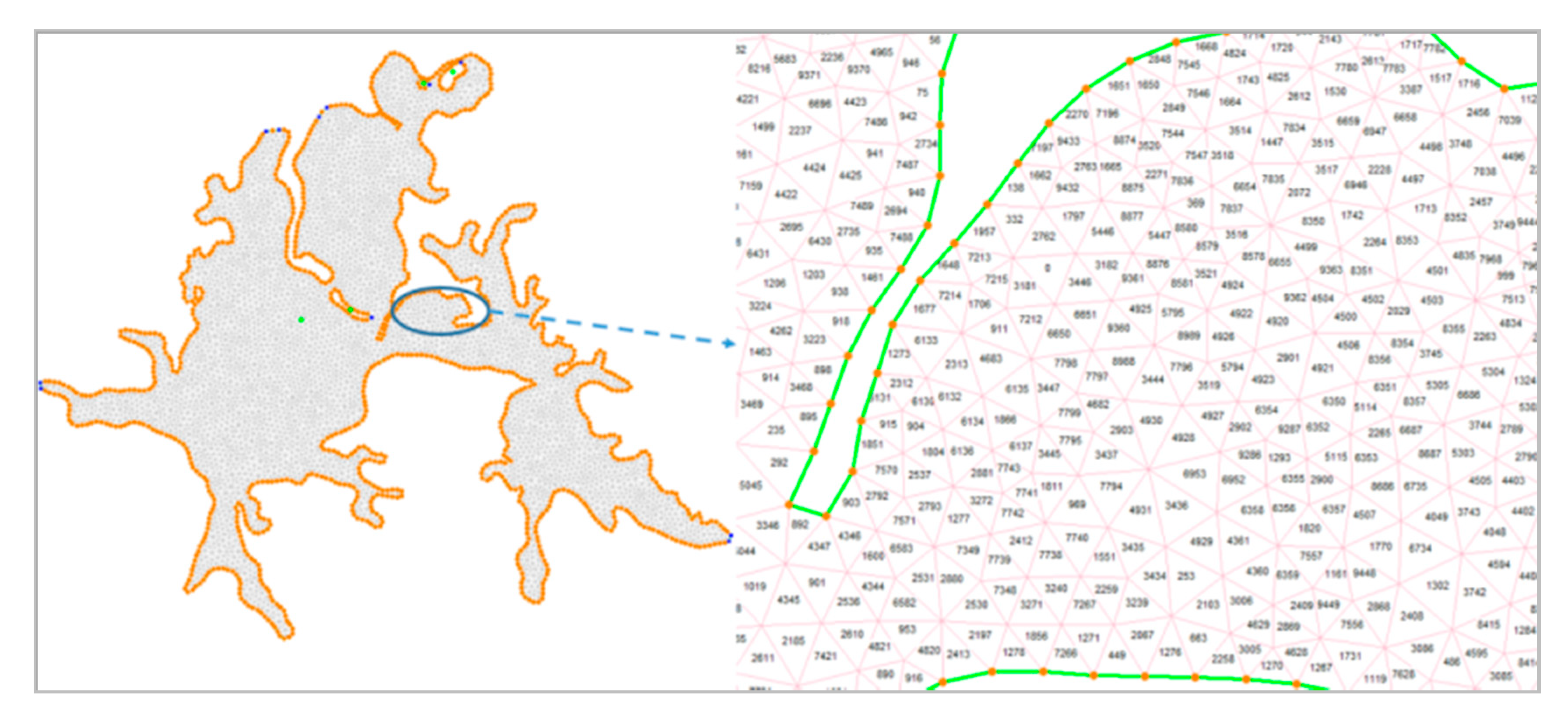
In this study, an unstructured triangular mesh was used to divide the terrain area of Donghu Lake. The specific division process included the selection of a simulation area, the determination of the terrain grid resolution, the definition of the open boundary in the land boundary, mesh generation, smoothing, and the calculation of the terrain difference. The result of the triangular mesh division is shown in Figure 6.
The required terrain boundary data comes from the pre-processing of GIS vector data from Donghu Lake. After the topographic boundary was introduced, the boundary vertex was redistributed (according to the actual situation of the Donghu Lake basin; the interval between the two vertices was determined to be 80 m) and the boundary was smoothed. In the end, the maximum area and minimum angle of the grid were defined as 5000 m2 and 30 m2 respectively, in order to avoid an unqualified regional triangular mesh. After saving the settings, it was run to generate the unstructured grid computing domain of the Donghu Lake basin (11,823 triangular computing units and 6462 grid vertices). Then, by smoothing the triangular grid domain (60 smoothing iterations) the local units were optimized and the triangles of the grid became as close as possible to equilateral triangles. On this basis, the binary bathymetric data was imported, and the natural neighborhood method (which provides a smoother approximation to the base “real” function and is more advantageous than the nearest neighbor interpolation method) was adopted for the bathymetric interpolation processing. Finally, the mesh was locally optimized and refined according to the water depth data to obtain the complete unstructured triangular mesh domain of Donghu Lake.
4.2.2. Initial Boundary Condition
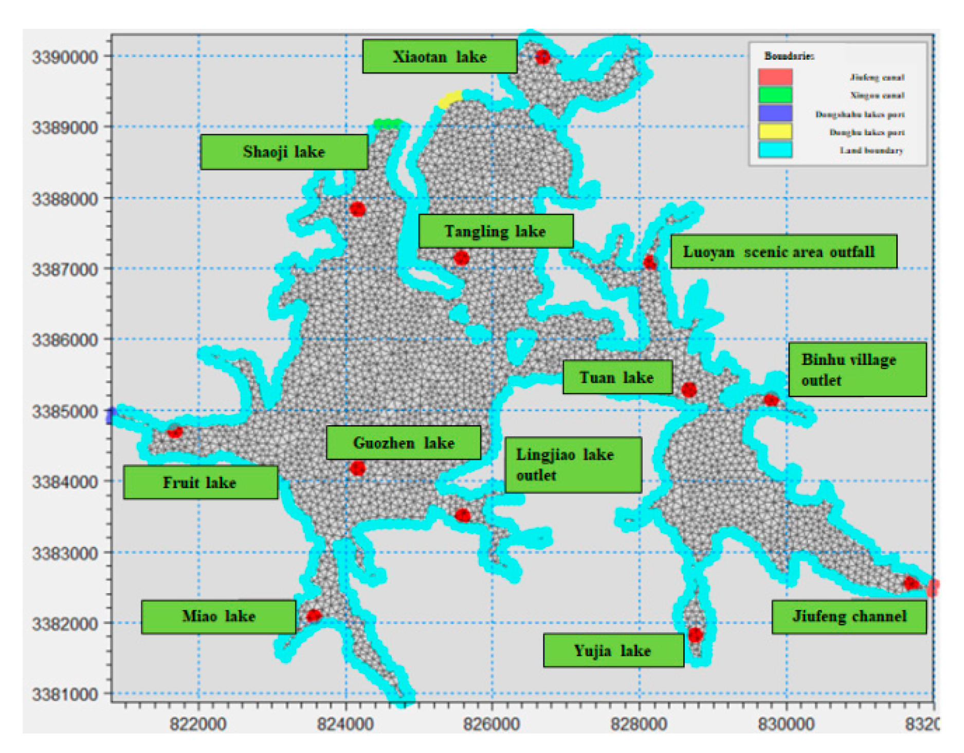
The simulation period was defined as from 00:00 h on 15 November 2017 to 00:00 h on 17 December 2017; a total of 32 days. The initial water level value was set as the annual average water level value of Donghu Lake (19.15 m), and the initial flow rate was set as 0 m/s. With reference to the optimal water diversion scheduling scheme in “The feasibility research report on the Donghu Lake Ecological Water Network Project in Wuhan city, Hubei province” [21], Qingshan port on the northwest side of the Donghu Lake and Zengjia alley on the southwest side were taken as the diversion gates. The Dongshahu canal and Donghu port were the inlet of the lake; the Xin ditch and the Jiufeng canal were the outlets for setting the hydrodynamic boundary.
The corresponding locations of the above-mentioned places were set as the open boundary. Donghu port and the Dongshahu canal were set as the open boundary of the inlet water (Code values of 2 and 3), and the Jiufeng canal and the Xin ditch were set as the open boundary of the outlet water (Code values of 4 and 5). The initial conditions were set for each triangular mesh in the simulation of the hydrodynamic model.
The boundary types were mainly divided into flow boundary and water level boundary. The time series recorded values of the water level boundary mainly came from the water and rain information inquiry system of Hubei province, and the data bulletin of the Wuhan Hydrologic Survey Bureau.
Since the research period was winter, it is not known whether the flow of diversion and drainage was implemented in strict accordance with the optimization scheme, so it was set as the water level boundary treatment. The water level data is difficult to obtain accurately in a long time series, because of the scarcity of water level stations in Donghu Lake. In this study, some boundary points were processed by MIKE interpolation according to the average water level value, and the model was input in DFS1 data format.
4.2.3. Parameter Setting
The main parameters set in the hydrodynamic model included the formula of the governing equation, the water depth of the dry and wet boundary, the lake bottom roughness coefficient, the Manning coefficient, the wind action (mainly the wind speed and direction), the source and sink flow, and the time series data. The fast first-order precision method in the hydrodynamic shallow water equation was selected. The main time step length of the model simulation was 2 h (7200 s); the total time step number was 384 times; and the value of the Courant number (CFL) was set as 0.85. There are dry and wet boundaries in the model area, which were set as the default parameter value (dry water depth was 0.005 m; submerged water depth was 0.05 m; and wet water depth was 0.1 m). The horizontal eddy viscosity coefficient was set as the default value of the Smagorinsky coefficient of MIKE21 (0.28).
The wind data came mainly from the global meteorological website (NOAA website) from November 15 to December 17. The weather station located near Donghu Lake on the north side of the Yangtze River was selected (monitoring every 3 h; partial missing data and abnormal data were supplemented and corrected according to historical queries of the China meteorological network). Available data included wind speed and direction, which were entered into the model in binary DFS0 file format. The wind friction was set as a function of the wind speed.
where is the air density. is the air drag force. is wind speed. = () is the wind speed measured at 10 m above sea level.
The boundaries of the source and sink terms were set during the water quality simulation. The specific hydrodynamic parameters are shown on Table 3.
4.2.4. Calibration and Validation of Model Parameters
After the above parameters were set, the hydrodynamic numerical model was run, and the results output in 2d plane sequence file format (DFSU). The MIKE data extraction tool was used to extract information on the specified verification point from the output result for model validation and parameter calibration. The water outlet of the Xin ditch in Donghu Lake was selected as the verification point. The water level and velocity values measured at the selected site were verified (referring to the data published by Hubei hydrology bureau), and the MIKE plot composing tool was used for statistical analysis. The results are shown in Figure 7.
From the comparison between the actual and simulated velocity data shown on Figure 5, it can be seen that the trend of the simulated data is in line with reality, but the relatively small value leads to a large error. According to the calculation, the error is greater than 40%. The water level is in line with west-high east-low terrain trend of Donghu Lake, but there is an abnormally high water level at the Luoyan scenic spot. The model therefore needs parameter calibration. The velocity error could be corrected by reducing the friction force at the bottom of the lake, that is, increasing the constant value of the Manning coefficient (changed to 42) or decreasing the value of the eddy viscosity coefficient (0.29). The modified flow velocity verification results are shown on Figure 8, and the water level verification results are shown on Figure 9. As can be seen from the figures, the average relative error value of the water level is less than 15% and the average relative error value of the flow velocity is less than 25% from 17 December to 15 December (time step: 1 h). The simulation effect basically conforms to the actual situation of free flow on the surface of Donghu Lake.
4.3. Water Quality Numerical Simulation of Donghu Lake by Remote Sensing Inversion
4.3.1. Basic Setting
(1) Initial boundary conditions settings
The pollutants in Donghu Lake mainly come from the surrounding inhabited areas, including point source pollution, non-point source pollution, and endogenous pollution. The non-point source pollution mainly comes from external pollutants carried in by rainfall, runoff, atmospheric deposition, and so on. The endogenous pollution mainly arises due to pollutant release from the bottom sediment and the bait pollution of the fishermen’s aquatic-breeding. Because this simulation work was carried out over a relatively short time and close to winter, Donghu Lake was in a dry period lacking rain. The point source pollution term was mainly established as a boundary condition of water quality, eliminating the non-point source pollution caused by rainfall and atmospheric deposition. Non-point source pollution was calculated according to land use, rainfall and runoff information around the lake, which required the collection of high quality data. According to the sewage outlet report of Wuhan Urban Drainage Development Ltd. and the Wuhan city water quality report, there are two existing large sewage treatment plants in Donghu Lake. These are the Lubuzui sewage plant and the Longwangzui (Jiufeng open channel) sewage plant, with additional small peripheral sewage treatment stations mainly distributed in the southwest area of Donghu Lake. In this study, following the actual situation of each sub-lake and its corresponding water quality index data in the simulation period, the point source pollution in Donghu Lake was first generalized into 7 sewage sources. According to the 2017 data bulletin of the lake water environment monitoring department of Wuhan city [22] and the existing investigation data [23], the load estimation values of each pollution index (including COD, BOD, TP and TN) at the generalized pollution source were obtained.
The water quality module (WQ) of the ECO Lab model was used in this study to simulate the water quality of Donghu Lake, and the indexes of this model included BOD, chlorophyll a, DO, nitrate nitrogen, orthophosphate phosphorus, and so on. The measuring cost of nitrate nitrogen and orthophosphate were high, so we determined the proportion (TP and TN) in the pollution load index (nitrate nitrogen accounts for 20% and orthophosphate accounts for 25%) based on existing research results [24], so as to determine the set value and input it to the water quality model. In addition, the boundary conditions and initial concentrations of pollution indicators for each source and sink term were set in combination with the measured concentration value (BOD, chlorophyll a, DO) of the Donghu Lake water quality index on 15 November, 2016.
(2) Parameter setting
Based on the completed hydrodynamic model (FM), modelling WQ with nutrients and chlorophyll, a template of the ECO Lab water quality model was added. Chlorophyll a, nitrate nitrogen and nitrite were selected as the main indicators for water quality simulation. The simulation started on 15 November 2017, with a time step of 2 h and an interval of 384 steps. Among them, the setting of the pollutant diffusion and degradation coefficients, as well as some constant parameters and force parameters, refer to historical empirical values [25]; the specific values are shown in Table 4.
(3) Model calibration and validation
The parameter calibration of the water quality numerical model mainly consisted of adjusting the diffusion coefficient, attenuation coefficient and the related biochemical reaction rate of the pollution parameter based on the simulation results. After the initial setting of the above parameters, the water quality simulation for the Donghu lake study period (model running time of 75 min) was conducted to obtain the simulation results of the concentration of the main water pollution index (chlorophyll a, nitrate nitrogen, ammonia, orthophosphate phosphorus) and the hydrodynamic flow field. Based on comprehensive analysis, the simulation results of chlorophyll a showed a large error, and the simulation results of nitrate nitrogen and orthophosphate phosphorus were in relatively good agreement with the actual situation, but there were also large local spatial variations. The reason may be that the water quality diffusion rate was set too high and the pollutant degradation rate too low. It was, therefore, necessary to re-calibrate the main parameters of the coupling model, and the final results are shown on Table 5.
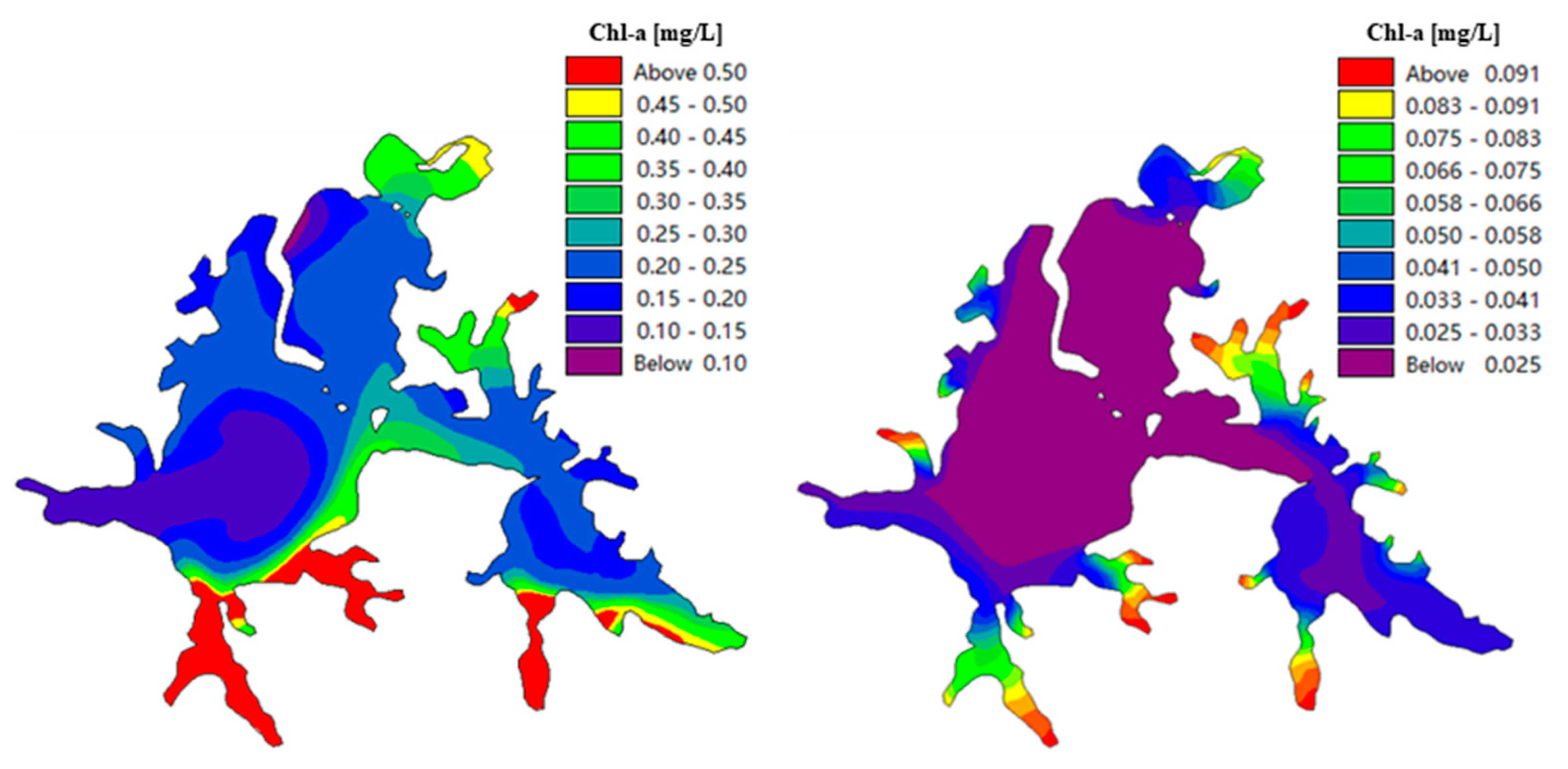
With chlorophyll a as a reference, the simulation effect after parameter calibration was analyzed. The comparison results are shown in Figure 10. The simulation results after parameter calibration were compared to those before, and the spatial information was improved to some extent. The simulation results near Fruit Lake and Liyuan hospital were consistent with the spatial distribution in the actual region.
The concentration range in some local areas has been corrected because the simulation results in Miaohu, Yujia Lake, and elsewhere were far beyond the actual range. The simulation calibration accords well with the actual situation.
4.3.2. Settings Optimization Based Remote Sensing
(1) Optimization of water quality initial concentration field based on remote sensing inversion
In this study, TN-measured data in Donghu Lake on 15 November and 17 December were used to test and verify the GA-BP regression model (BP neural network remote sensing inversion model optimized by the GA). The results of the regression statistics show that the correlation coefficient (R) = 0.88, the determinant coefficient (R2) = 0.78, and the root-mean-square error (RMSE) = 1.49. The simulation accuracy meets the requirements. It was, therefore, applied to the inversion of total nitrogen concentration in Donghu Lake to obtain the distribution of the initial concentration field. The results show that the overall spatial distribution of TN inversion concentration is reasonable, and each sub-lake region is consistent with the actual situation, which verifies the reliability of the model. The statistical result is shown in Figure 11. Based on this, the spatial initial concentration field of the TN was obtained.
(2) Optimization of pollution source based on remote sensing
Point source pollution has a great influence on the water quality of Donghu Lake. The setting of pollution sources in the numerical model is also very important for the simulation results. The more detailed the source information, the more accurate and reliable the simulation results will be. Therefore, while supplementing the initial background concentration field, inversion results can also be used to enrich local pollution source information, as shown in Figure 12. The number of spatially generalized pollution sources increased from 7 to 13. Among them, most of the supplementary pollution sources are representative areas with severe water pollution; the previously measured data are limited and cannot be specifically covered.
(3) Initial condition optimization of the water quality model based on remote sensing
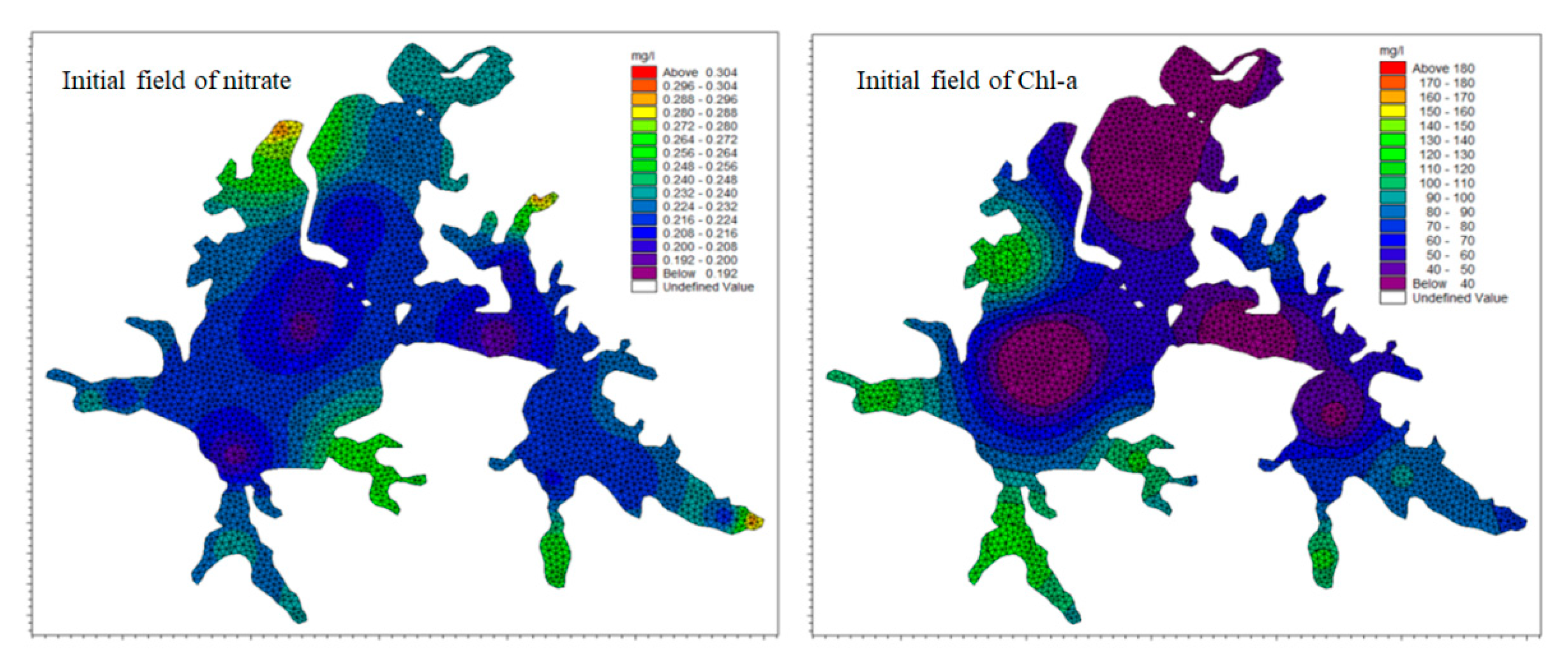
The indexes of water quality, chlorophyll a and nitrate nitrogen were taken as the main supplementary data. Remote sensing inversion was used to obtain the water quality index concentration value at the initial time of the model as the initial field of this index.
The ArcGIS element editing tool was used to select the corresponding water quality index density values of each typical region to obtain the optimal remote sensing inversion data of the initial stage of the simulation (15 November 2017) according to their spatial distribution. This was input into the synchronization region of the MIKE calculation surface domain (DFSU), and local interpolation processing was conducted to supplement and improve the initial concentration field of the two water quality indicators, as shown in Figure 13.
5. Results and Discussion
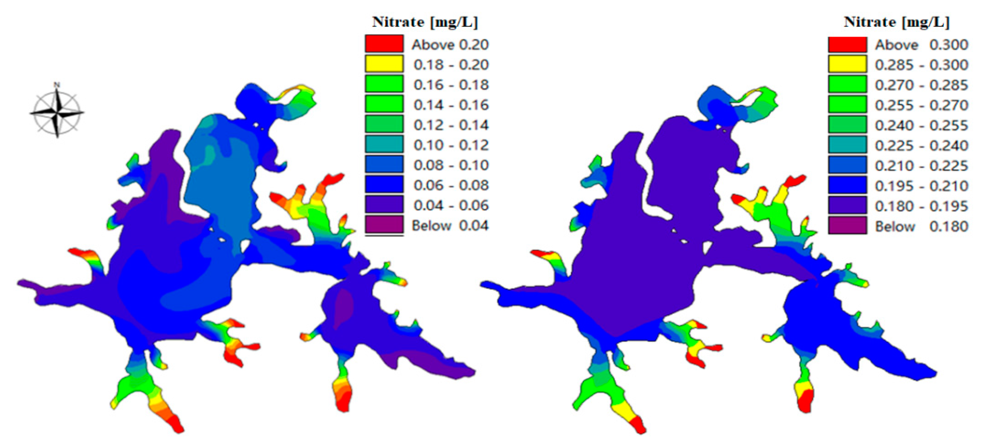
The hydrodynamic and water quality simulation process was completed by using data optimized both with and without remote sensing data. The horizontal comparison was then performed (see Figure 14).
The main eutrophication indicators (chlorophyll a and nitrate nitrogen) were selected for analysis, and the verification statistical results are shown on Table 4.
From the spatial distribution of the results in Figure 11 and Table 6 above, the simulation results of the water quality model were spatially optimized after the increase of the initial background concentration field and pollution source information. The local information was more abundant and the distribution was more reasonable, making up for the influence of the model error caused by the lack of measured values in some areas. Table 7 shows the average relative error values of 13 recalculated verification points. It can be seen in the calculation results that the average relative error of the water quality model simulation became smaller after the data supplement with inversion. The MSE of the chlorophyll a simulation decreased from 19% to 17%, and the MSE of nitrate nitrogen simulation decreased from 31% to 24%. The accuracy of the model was improved and the outliers in the original model were corrected to some extent. For example, the relative error of nitrate nitrogen simulation at the Yujiahu verification point decreased from 71% to 11.5%. The calculated results demonstrate the feasibility of remote sensing inversion to optimize water quality simulation from a statistical perspective, indicating that the inversion data is suitable for supplementary optimization of the model in the absence of measured data.
6. Conclusions
In this study of Donghu Lake, a heuristic intelligent algorithm has been applied in the field of empirical remote sensing inversion, and an improved BP neural network algorithm model based on the genetic algorithm (GA) is proposed. On the basis of the measured water quality and spectral data from Donghu Lake, the nonlinear regression fitting relationship between the measured data of chlorophyll a and the spectral reflectance of the wave band was established using the optimization algorithm, and the inversion model of chlorophyll a concentration in Donghu Lake water was established. The statistics show that the simulation results of the model have greater accuracy, and the inversion model has higher adaptability to the generalization of each period of data. This can be applied to the overall inversion of chlorophyll a concentration in the water quality of Donghu Lake.
The numerical simulation results of water quality based on the traditional measured data are insufficient, and the simulation results are poor in spatial information. The water quality simulation results obtained using the GA-BP remote sensing inversion model have spatial optical sensitivity, and can reasonably show the regional distribution of water quality index concentrations in Donghu Lake. On this basis, combining the advantages of the two, chlorophyll a and nitrate nitrogen indexes were selected, and the areas lacking measured data were supplemented by inversion values. After the optimization, the simulated MSE of the chlorophyll a index decreased to 17.8%, and the MSE of nitrate nitrogen decreased to 24.9. Moreover, the local anomaly error was corrected, and the spatial simulation results are more reasonable. The feasibility of combining remote sensing inversion with water environment numerical simulation and optimizing the results was verified.
Author Contributions
Conceptualization: X.L.; funding acquisition: M.H.; methodology: R.W.; model: R.W.; writing—original draft: X.L.; writing—review and editing: M.H. All authors have read and agreed to the published version of the manuscript.
Funding
This research was funded by the National Natural Science Foundation of China (No. 51579108), the National Key R and D Program of China (No. 2017YFC0405901).
Conflicts of Interest
The authors declare no conflict of interest.
References
- Song, N.; Bai, L.; Xu, H.; Jiang, H. The composition difference of macrophyte litter-derived dissolved organic matter by photodegradation and biodegradation: Role of reactive oxygen species on refractory component. Chemosphere 2020, 242, 125155. [Google Scholar] [CrossRef] [PubMed]
- Qin, B.; Gao, G.; Zhu, G.; Zhang, Y.; Song, Y.; Tang, X.; Xu, H.; Deng, J. Lake eutrophication and its ecosystem response. Chin. Sci. Bull. 2013, 58, 961–970. [Google Scholar] [CrossRef] [Green Version]
- Weichun, M.A.; Zhang, C. The Numerical Simulation of Water Quality of Suzhou Creek Based on Gis. Acta Geographica Sinica 1998, 53 (Suppl. 6), 66–75. [Google Scholar]
- Xiao, C.; Liang, X.; Du, C.; Xie, S.; Fang, Z.; Ma, Z.; Feng, B.; Tian, Z. Numerical Simulation and Improvement Measures of Water Quality in Yangshapao Lake. In Proceedings of the 2009 3rd International Conference on Bioinformatics and Biomedical Engineering, Beijing, China, 11 June 2009; pp. 1–4. [Google Scholar]
- Mano, A.; Malve, O.; Koponen, S.; Kallio, K.; Taskinen, A.; Ropponen, J.; Juntunen, J.; Liukko, N. Assimilation of satellite data to 3D hydrodynamic model of Lake Säkylän Pyhäjärvi. Water Sci. Technol. 2015, 71, 1033–1039. [Google Scholar] [CrossRef] [PubMed]
- Peng, S.; Fu, G.; Zhao, X.; Moore, B.C. Integration of environmental fluid dynamics code (EFDC) model with geographical information system (GIS) platform and its applications. J. Environ. Inform. 2011, 17, 75–82. [Google Scholar] [CrossRef]
- Jia, H.; Zhang, Y.; Guo, Y. The development of a multi-species algal ecodynamic model for urban surface water systems and its application. Ecol. Model. 2010, 221, 1831–1838. [Google Scholar] [CrossRef]
- Wu, G.; Xu, Z. Prediction of algal blooming using EFDC model:Case study in the Daoxiang Lake. Ecol. Model. 2011, 222, 1245–1252. [Google Scholar] [CrossRef]
- Huang, M.; Tian, Y. An Integrated Graphic Modeling System for Three-Dimensional Hydrodynamic and Water Quality Simulation in Lakes. ISPRS Int. J. Geo-Inf. 2019, 8, 18. [Google Scholar] [CrossRef] [Green Version]
- Safaa, H.; Esam, I. Detection and Evaluation of Groundwater in Siwa Oasis, Egypt Using Hydrogeochemical and Remote Sensing Data Analysis. Water Environ. Res. 2018, 90, 465–478. [Google Scholar] [CrossRef] [PubMed]
- Zhou, Q.; Tian, L.; Wai, O.W.; Li, J.; Sun, Z.; Li, W. High-Frequency Monitoring of Suspended Sediment Variations for Water Quality Evaluation at Deep Bay, Pearl River Estuary, China: Influence Factors and Implications for Sampling Strategy. Water 2018, 10, 323. [Google Scholar] [CrossRef] [Green Version]
- Koponen, S.; Pulliainen, J.; Kallio, K.; Hallikainen, M. Lake water quality classification with airbrone hyperspectral specyrometer and simulated MERIS data. Remote Sens. Environ. 2002, 79, 51–59. [Google Scholar] [CrossRef]
- Zhu, Y.; Zhu, L.; Li, J.; Chen, Y.; Zhang, Y.; Hou, H.; Ju, X.; Zhang, Y. The study of inversion of chlorophyll a in Taihu based on GF-1 WFV image and BP neural network. Acta Scientiae Circumstantiae 2017, 37, 130–137. [Google Scholar]
- Shi, R.; Zhang, H.; Yue, R.; Zhang, X.; Wang, M.; Shi, W. A wavelet theory based remote sensing inversion of chlorophyll a concentrations for inland Lakes in arid areas using TM image data. Acta Ecol. Sin. 2017, 37, 1043–1053. [Google Scholar]
- Cao, Y.; Ye, Y.; Zhao, H.; Jiang, Y.; Wang, H.; Wang, J. Ensemble modeling methods for remote sensing retrieval of water quality parameters in inland water. China Environ. Sci. 2017, 37, 3940–3951. (In Chinese) [Google Scholar]
- Wang, J.; Cheng, S.; Jia, H.; Wang, Z.; Tang, U. An Artificial Neural Network Model for Lake Color Inversion Using TM Imagery. Environ. Sci. 2003, 24, 73–76. (In Chinese) [Google Scholar]
- Chang, N.B.; Xuan, Z.; Yang, Y.J. Exploring spatiotemporal patterns of phosphorus concentrations in a coastal bay with MODIS images and machine learning models. Remote Sens. Environ. 2013, 134, 100–110. [Google Scholar] [CrossRef]
- Hajigholizadeh, M.; Melesse, A.M.; Fuentes, H.R. Erosion and Sediment Transport Modeling in Shallow Waters: A Review on Approaches, Models and Applications. Int. J. Environ. Res. Public Health. 2018, 15, 518. [Google Scholar] [CrossRef] [PubMed] [Green Version]
- Chen, Q.; Huang, M.; Tang, X. Eutrophication assessment of seasonal urban Lakes in China Yangtze River Basin using Landsat 8-derived Forel-Ule index: A six-year (2013–2018) observation. Available online: https://0-www-sciencedirect-com.brum.beds.ac.uk/science/article/pii/S0048969719353859 (accessed on 22 April 2019).
- Luo, Y.X. Research progress on environmental quality of water resources in Donghu Lake of Wuhan. J. Green Sci. Technol. 2018, 58–60. (In Chinese) [Google Scholar]
- Hubei Water Resources and Hydropower Survey and Design Institute. Feasibility study report on construction of water network connection project of dadong Lake ecological water network in wuhan, hubei province. M Environ. Study Monit. 2010. (In Chinese) [Google Scholar]
- Wuhan Bureau of Ecology and Environment. Environmental Quality of Surface Water in Wuhan in December 2017. Available online: http://hbj.wuhan.gov.cn/hbDbsjcbg/28411.jhtml73107479-1/2018-00058 (accessed on 17 April 2019).
- Guo, X.R. Water Quality Simulation of East Lake in Wuhan City Based on Hydrodynamics. Master’s Thesis, Xi’an University of Technology, Xi’an, China, 2018. (In Chinese). [Google Scholar]
- Jing, Z. Numerical Simulations of the Lake Water Environment and Parallel Computations of the Non-hydrostatic Flows. Available online: http://gb.oversea.cnki.net/KCMS/detail/detail.aspx?filename=1017145957.nh&dbcode=CDFD&dbname=CDFDREF (accessed on 12 April 2019).
- Li, X. The Mechanism of Nitrogen Migration and Transformation in Shallow Lake Sediments. Ph.D. Thesis, Tianjin University, Tianjin, China, 2012. (In Chinese). [Google Scholar]
Figure 1.
Genetic algorithm (GA)-optimized back propagation (BP) algorithm flow.
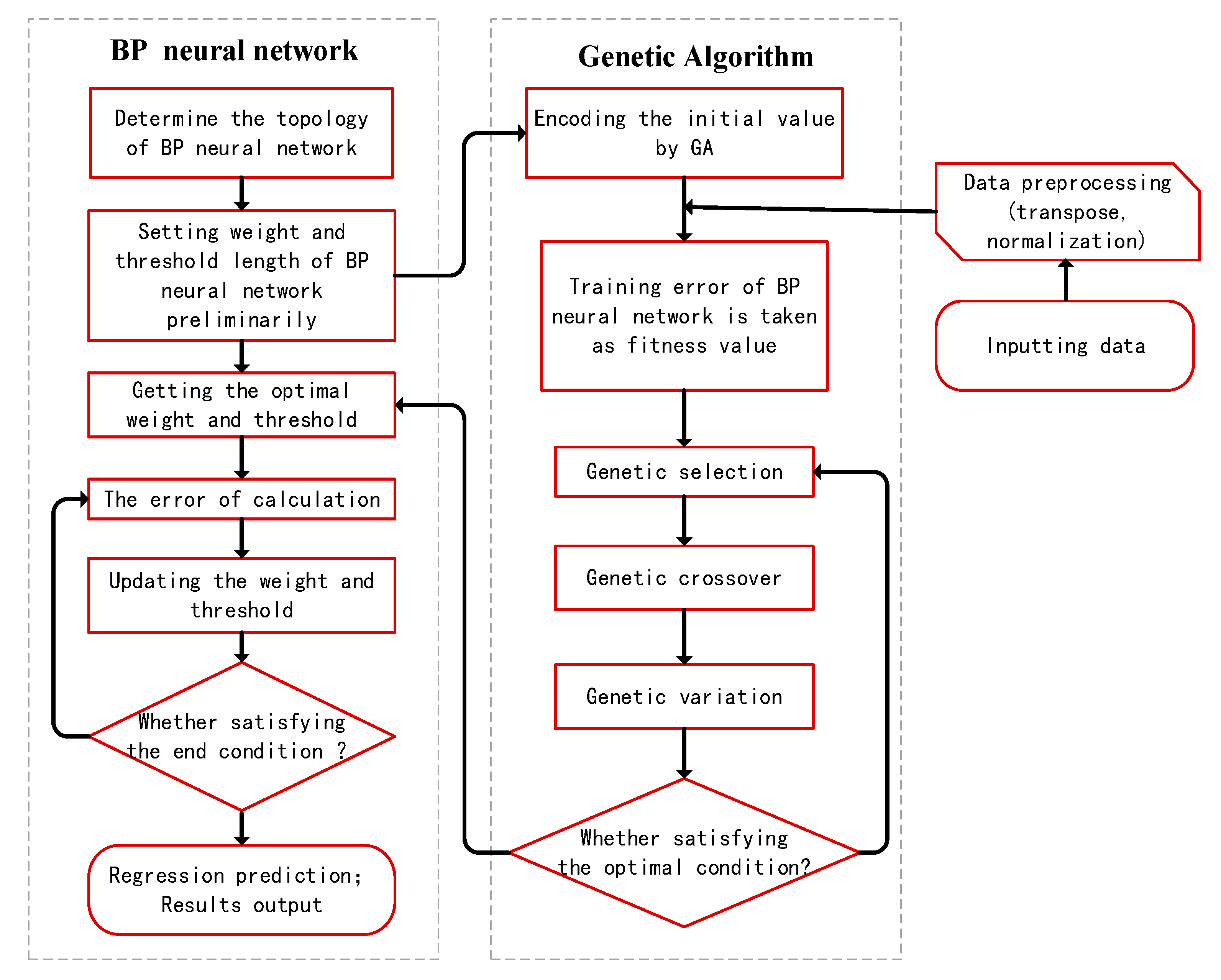
Figure 2.
Arrangement diagram of Donghu Lake sampling.

Figure 3.
Regression statistics results (top) and Simulation result (bottom).
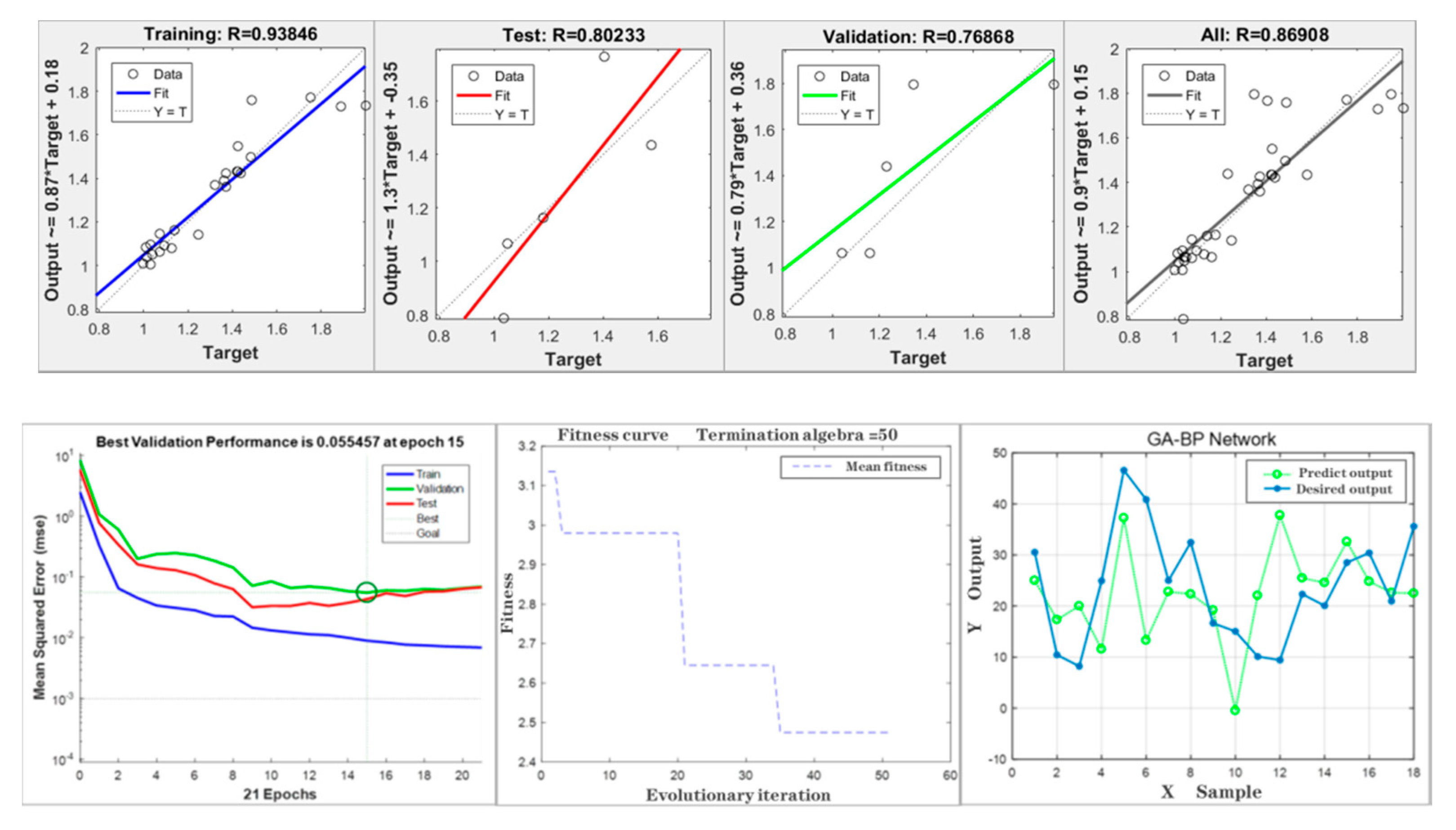
Figure 4.
Chlorophyll a concentration inversion distribution on 15 November 2017 in Donghu Lake.

Figure 5.
Chlorophyll a concentration inversion distribution on 17 December 2017 in Donghu Lake.

Figure 6.
Results of Donghu Lake unstructured triangular meshes.

Figure 7.
Verification of the comparison of point velocity data.
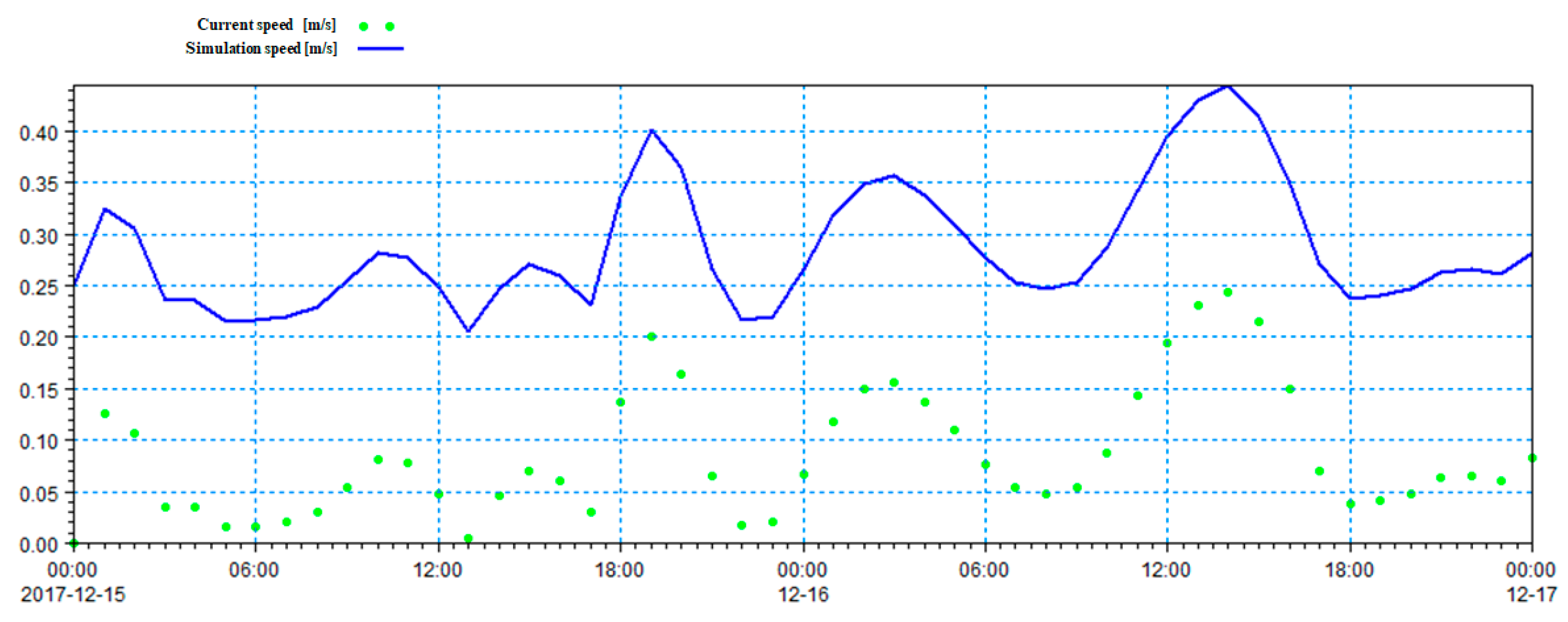
Figure 8.
Results of flow rate verification at Xin ditch station.
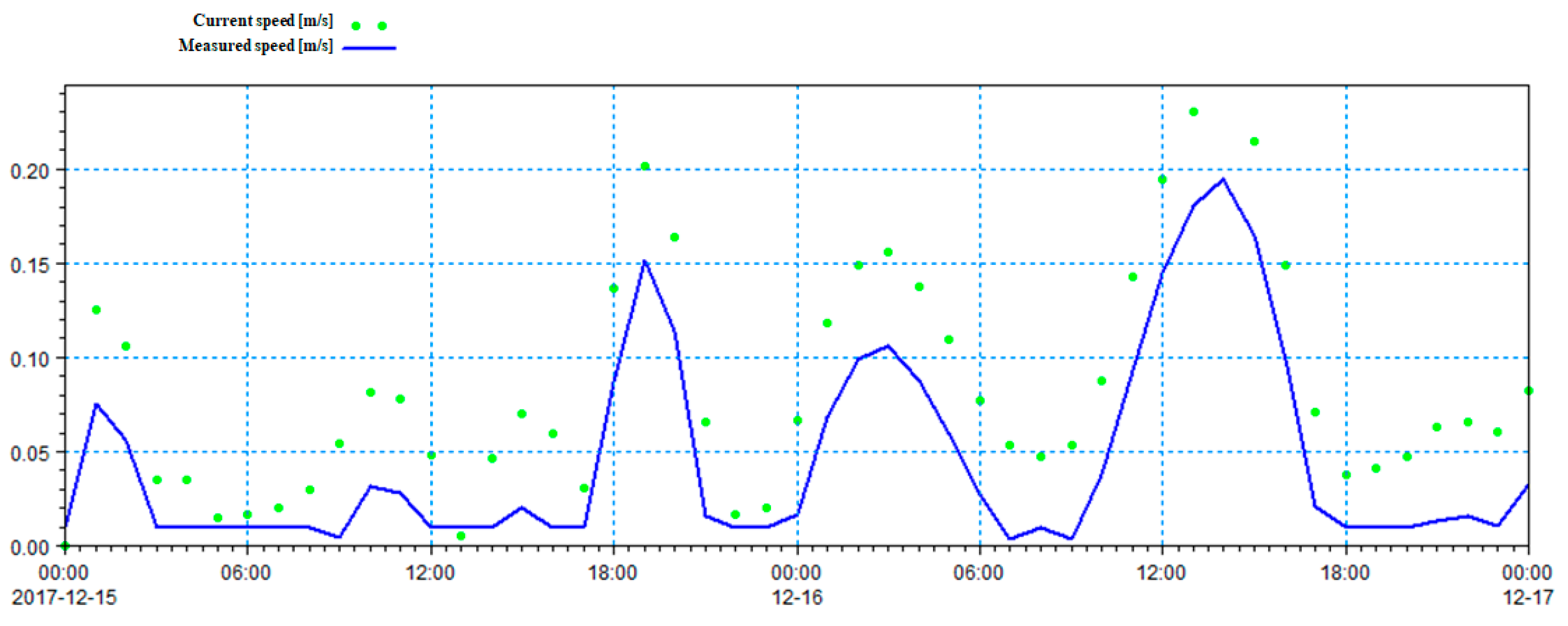
Figure 9.
Water level verification results at Xin ditch station.
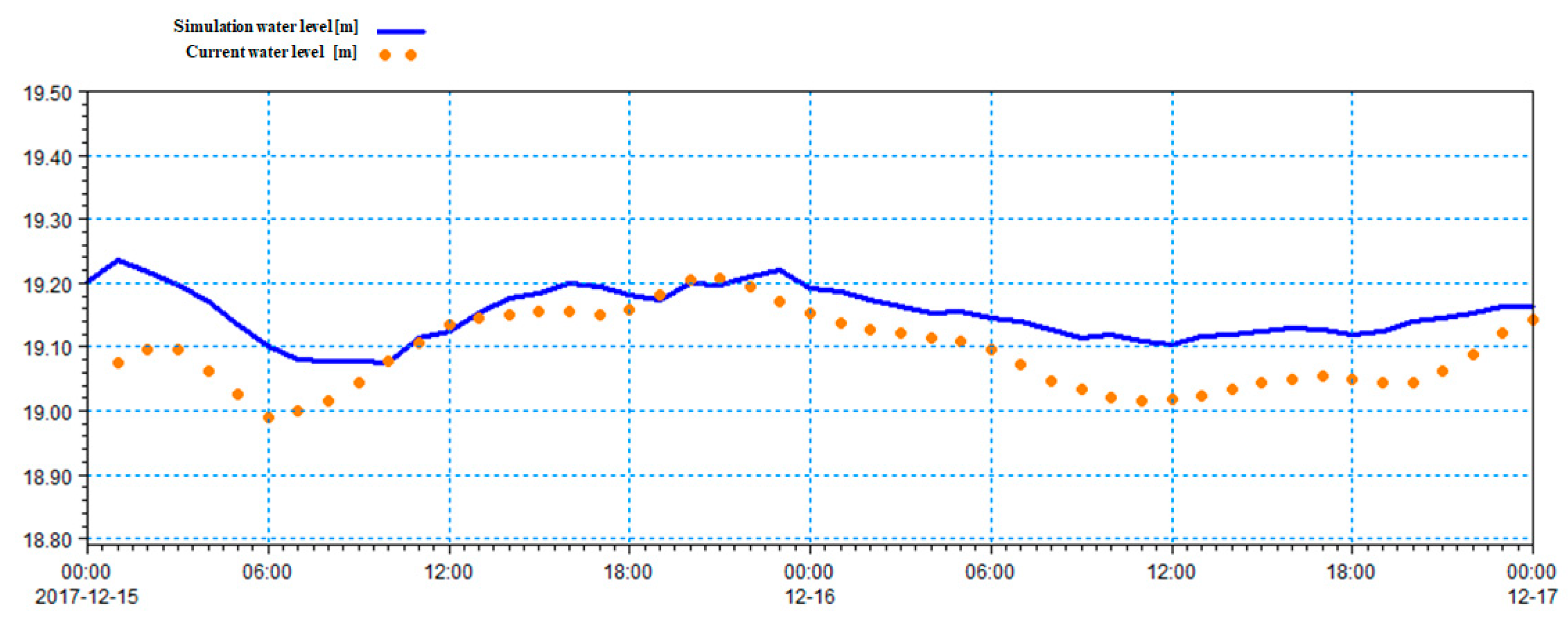
Figure 10.
Comparison of chlorophyll a simulation results before (left) and after (right) parameter calibration.
Figure 10.
Comparison of chlorophyll a simulation results before (left) and after (right) parameter calibration.

Figure 11.
Simulated statistical results of total nitrogen (TN).
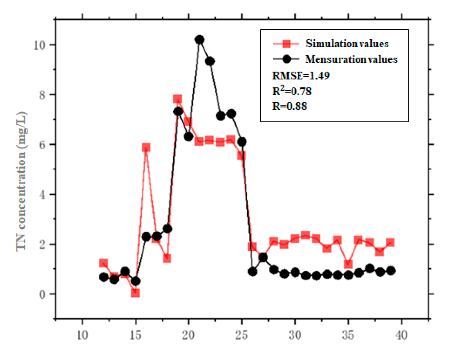
Figure 12.
Supplementary results of pollution sources.

Figure 13.
Replenishment of initial concentration field.

Figure 14.
Comparison of nitrate simulation results based (left) and not based (right) on remote sensing optimization.
Figure 14.
Comparison of nitrate simulation results based (left) and not based (right) on remote sensing optimization.


Table 1.
Measured water quality data of Donghu Lake (2017.12).
| Point | Northern Latitude | East Longitude | PH | Turbidity (NTU) | TP (mg/L) | TN (mg/L) | DO | Chlorophyll a (mg/m3) | CODcr (mg/L) |
|---|---|---|---|---|---|---|---|---|---|
| 1 | 30.553 | 114.397 | 6.850 | 19.980 | 0.126 | 0.538 | 10.22 | 22.201 | 10.566 |
| 2 | 30.560 | 114.398 | 7.470 | 22.600 | 0.095 | 2.782 | 10.45 | 15.690 | 15.094 |
| 3 | 30.565 | 114.402 | 7.600 | 12.160 | 0.097 | 1.134 | 10.36 | 5.814 | 18.113 |
| 4 | 30.581 | 114.407 | 7.660 | 56.700 | 0.190 | 1.005 | 10.35 | 5.978 | 13.585 |
| 5 | 30.590 | 114.405 | 7.810 | 31.400 | 0.166 | 1.658 | 10.31 | 5.246 | 15.094 |
| 6 | 30.584 | 114.401 | 7.620 | 11.180 | 0.094 | 1.372 | 10.22 | 6.695 | 10.566 |
| 7 | 30.586 | 114.391 | 7.760 | 24.500 | 0.128 | 1.980 | 10.27 | 6.771 | 18.113 |
| 8 | 30.573 | 114.394 | 7.790 | 12.980 | 0.111 | 1.933 | 10.47 | 10.996 | 27.170 |
| 9 | 30.564 | 114.395 | 7.890 | 48.500 | 0.174 | 0.745 | 10.52 | 6.971 | 34.717 |
Table 2.
The basic parameters of the model Settings.
| GA | BP | ||
|---|---|---|---|
| Name of Parameter | Set Value | Name of Parameter | Set Value |
| Population size (20~100) | 8 | Number of nodes in input layer | 7 |
| Generation number of training (100~1000) | 50 | Number of nodes in hidden layer | 4 |
| Crossover probability (0.4~0.9) | 0.3 | Number of nodes in output layer | 1 |
| Mutation probability (0.0001~0.1) | 0.1 | Maximum iterations | 1000 |
| Objectives of training | 0.001 | ||
| Output function in hidden layer | Tansig | ||
| Output function in output layer | Purelin | ||
| Training function | Trainlm | ||
Table 3.
Hydrodynamic model parameter setting.
| Parameter | Value |
|---|---|
| Solution Technique | Low order, fast algorithm |
| Depth | No depth correction |
| Flood and Dry | Standard flood and dry |
| Density | Barotropic |
| Eddy Viscosity | Smagorinsky constant value (0.32) |
| Bed Resistance | Manning constant (35 m1/3/s) |
| Coriolis Forcing | Varying in Domain |
| Wind Forcing | Time varying spatial constant |
| Initial Condition | The mean water level (19.05 m), Flow velocity (0 m/s) |
| Boundary Condition | Water level boundary (import DFS1 file) |
Table 4.
Some parameters settings of the water quality model.
| Parameter Name | Set Point |
|---|---|
| Degradation rate at 20 °C of BOD | 0.5 (/d) |
| Temperature coefficient of BOD | 1.07 dimensionless |
| Consumes oxygen half-saturation constant in process of BOD degradation | 2 mg/L |
| Oxygen rate of aquatic plants | 0 (/d) |
| The temperature coefficient in the process of oxygen consumption | 1.08 dimensionless |
| Half-saturation constant in the process of oxygen consumption | 2 mg/L |
| Oxygen consumption per square meter of mud | 0.5 (/d) |
| Half-saturation constant—The ammonia nitrogen in photosynthesis | 0.066 gNH4/g BOD |
| Half-saturation constant—The absorbed orthophosphates in photosynthesis | 0.015 gP/g BOD |
| Chlorophyll a decay rate | 0.01 (/d) |
| Nitrification rate | 0.05 (/d) |
| Nitrification oxygen demand (NH4-NO2) | 3.42 gO2/g NH4-N |
| Nitrification oxygen demand (NO2 ~ NO3) | 1.14 gO2/g NO2-N |
| Attenuating release phosphorus content of BOD | g P/g BOD |
| Temperature | 11.04 degrees C |
| Salinity | 95 psu |
| Transverse and longitudinal diffusion coefficients | 6.2 m2/s |
Table 5.
The calibrated parameter values of the coupling model.
| Parameter Name | Parameter Values |
|---|---|
| Smagorinsky Eddy viscosity coefficient | 0.29 |
| Manning constant | 42 m1/3/s |
| Coriolis force | It is automatically calculated with the latitude information of the surface area |
| Transverse and longitudinal diffusion coefficients | average 9.2 m2/s |
| Ammonia nitrogen degradation coefficient (20 °C standard) | 0.045 (/d) |
| Orthophosphate Phosphorus degradation coefficient (20 °C standard) | 0.035 (/d) |
| BOD attenuation coefficient (20 °C standard) | 0.025 (/d) |
| Chlorophyll a attenuation coefficient (20 °C standard) | 0.015 (/d) |
| Nitrification rate (20 °C standard) | 0.035 (/d) |
Table 6.
Contrastive analysis of the verify point mean square error (MSE) (%).
| Pollution Parameter | Simulated Result Not Based on Remote Sensing Optimization | Simulated Result Based on Remote Sensing Optimization |
|---|---|---|
| Chlorophyll a | 19.60 | 17.8093 |
| Nitrate nitrogen | 31.02 | 24.9610283 |
Table 7.
The error analysis after optimization based on inversion.
| Name of Lake | Chlorophyll a Measured Value (Mg/L) | Chlorophyll a Value of Simulation (Mg/L) | RE (%) | NO3-N Measured Value (Mg/L) | NO3-N Value of Simulation (Mg/L) | RE (%) |
|---|---|---|---|---|---|---|
| Tangling Lake | 0.01551 | 0.0240 | 54.6396 | 0.3150 | 0.1901 | 39.6489 |
| Shaoji Lake | 0.02532 | 0.0240 | 5.0569 | 0.1400 | 0.1902 | 35.8321 |
| Tuan Lake | 0.02625 | 0.0239 | 8.8301 | 0.1700 | 0.1900 | 11.7518 |
| Lingjiao Lake | 0.02525 | 0.0303 | 20.1192 | 0.2020 | 0.2245 | 11.1158 |
| Xiaotan Lake 2 | 0.01821 | 0.0243 | 33.5124 | 0.2920 | 0.1948 | 33.2877 |
| Fruit Lake | 0.02742 | 0.0255 | 6.9325 | 0.1780 | 0.1986 | 11.5781 |
| Guozhen Lake 1 | 0.02566 | 0.0239 | 6.6933 | 0.1200 | 0.1898 | 58.1617 |
| Yujia Lake | 0.05096 | 0.0516 | 1.2223 | 1.0600 | 1.1818 | 11.4925 |
| Xiaotan Lake 1 | 0.02816 | 0.0248 | 11.8487 | 0.1620 | 0.2014 | 24.3290 |
| Tiane Lake | 0.02241 | 0.0243 | 8.6158 | 0.1500 | 0.1919 | 27.9527 |
| Guozhen Lake 2 | 0.02176 | 0.0239 | 9.9508 | 0.1420 | 0.1897 | 33.6204 |
| Hou Lake | 0.04015 | 0.0247 | 38.5599 | 0.2140 | 0.2103 | 1.7107 |
| Miao Lake | 0.06256 | 0.0466 | 25.5400 | 0.4250 | 0.3229 | 24.0120 |
© 2020 by the authors. Licensee MDPI, Basel, Switzerland. This article is an open access article distributed under the terms and conditions of the Creative Commons Attribution (CC BY) license (http://creativecommons.org/licenses/by/4.0/).
Share and Cite
MDPI and ACS Style
Li, X.; Huang, M.; Wang, R. Numerical Simulation of Donghu Lake Hydrodynamics and Water Quality Based on Remote Sensing and MIKE 21. ISPRS Int. J. Geo-Inf. 2020, 9, 94. https://0-doi-org.brum.beds.ac.uk/10.3390/ijgi9020094
AMA Style
Li X, Huang M, Wang R. Numerical Simulation of Donghu Lake Hydrodynamics and Water Quality Based on Remote Sensing and MIKE 21. ISPRS International Journal of Geo-Information. 2020; 9(2):94. https://0-doi-org.brum.beds.ac.uk/10.3390/ijgi9020094
Chicago/Turabian StyleLi, Xiaojuan, Mutao Huang, and Ronghui Wang. 2020. "Numerical Simulation of Donghu Lake Hydrodynamics and Water Quality Based on Remote Sensing and MIKE 21" ISPRS International Journal of Geo-Information 9, no. 2: 94. https://0-doi-org.brum.beds.ac.uk/10.3390/ijgi9020094
Note that from the first issue of 2016, this journal uses article numbers instead of page numbers. See further details here.