Concept Lattice Method for Spatial Association Discovery in the Urban Service Industry

Abstract

A relative lag in research methods, technical means and research paradigms has restricted the rapid development of geography and urban computing. Hence, there is a certain gap between urban data and industry applications. In this paper, a spatial association discovery framework for the urban service industry based on a concept lattice is proposed. First, location data are used to form the formal context expressed by 0 and 1. Frequent closed itemsets and a concept lattice are computed on the basis of the formal context of the urban service industry. Frequent closed itemsets can filter out redundant information in frequent itemsets, uniquely determine the complete set of all frequent itemsets, and be orders of magnitude smaller than the latter. Second, spatial frequent closed itemsets and association rules discovery algorithms are designed and built based on the formal context. The inputs of the frequent closed itemsets discovery algorithms include the given formal context and frequent threshold value, while the outputs are all frequent closed itemsets and the partial order relationship between them. Newly added attributes create new concepts to guarantee the uniqueness of the new spatial association concept. The inputs of spatial association rules discovery algorithms include frequent closed itemsets and confidence threshold values, and a rule is confident when and only if its confidence degree is not less than the confidence threshold value. Third, the spatial association of the urban service industry in Nanning, China is taken as a case to verify the method. The results are basically consistent with the spatial distribution of the urban service industry in Nanning City. This study enriches the theories and methods of geography as well as urban computing, and these findings can provide guidance for location-based service planning and management of urban services.

1. Introduction

Spatial association and aggregation of the urban service industry are industry characteristics. Identifying these characteristics requires some methods based on spatial data [1]. Due to the rapid development of e-commerce, mainstream online platforms offer real-time data sources for all related subjects and provide geo-tagging data for geographic research [2,3,4]. Utilizing the public data of these e-commerce platforms to conduct urban computing based on big data, services for urban planning and management can be provided [5,6]. There is a certain gap between the big data and industry applications, and researchers need to find appropriate research methods to turn data into knowledge for the essence of research objectives and research questions [7]. The association analysis was developed from the classic "beer and diaper" story, presented by Agrawal [8]. Spatial association belongs to the category of association rule mining. Researchers can divide up spatial objects to generate a series of spatial neighborhoods and then find the frequent co-location subsets according to the neighborhood, thus discovering the spatial association mode [9]. There are many algorithms for association rules, which can generally be divided into several topics, such as frequent itemsets mining, frequent closed itemsets mining, the single largest set mining, parallel and distributed mining and so on [10]. There are various algorithms for frequent itemsets, and the number of frequent itemsets obtained by mining is often amazing. The Apriori algorithm is a representative algorithm of frequent itemset mining, which has some problems in efficiency due to too many scanning instances.

The spatial association rules themselves are vague and uncertain, and it is necessary to find a way to better deal with uncertain spatial data. The concept lattice, first proposed by Wille [11], provides an effective tool for analyzing the connection between objects and attributes. The concept lattice is used to express the frequent closed itemsets through the concept node to carry out association rule mining. Currently, its algorithm mainly consists of the a-close algorithm based on the Galois connection closure mechanism [12], the CLOSET algorithm based on Fp-tree [13], the CHARM algorithm using vertical data representation [14], the CLOSET+ algorithm using mixed projection strategy [15], the FPClose algorithm combining the Fp-tree data structure with an array, and other optimization strategies [16]. The concept lattice has some applications for industry in the present study. Zou used the concept lattice to set up the concept lattice recommendation system for separating online and offline parts [17]. Kuo used formal concept analysis and an association rule methodology to develop a Keyword Association Lattice [18]. The mathematical framework of the biological interpretation of gene expression data was established by Kim through a concept lattice [19]. In terms of spatial data application, Li put forward a type of spatial data weighted concept lattice framework and used Chinese basic geographic information data and spatial data in the field of water conservancy projects for example verification [20]. Using a concept lattice, Xie put forward three new types of rules: decision association rules, non-redundant decision association rules and simplest decision association rules [21]. Using the distance and membership degree of different index levels of spatial entities to measure the similarity of attributes, Liao proposed a spatial data attribute similarity measurement method based on granular computing closeness [22]. Sikder presented a granular computing approach to spatial classification and prediction of land cover classes using rough set variable precision methods [23]. The urban service industry has spatial characteristics. The urban commercial spatial distribution is characterized by significant agglomeration and has shown a polycentric distribution pattern [24]. A method to identify urban functional regions by combining point-of-interest data with floating car track data has been proposed [25].

These predecessors have conducted much work regarding the definition and calculation of spatial association, association algorithms, concept lattice definition and algorithms, urban spatial calculation, and so on. In the current study, we hypothesize the following: 1) there is a spatial association between the service industries in a city; 2) there should be a mathematical method to find the spatial association of the urban service industry; and 3) the concept lattice should be this method because it has some advantages over other methods. To test the hypotheses, we investigated spatial association clustering of the urban service industry in Nanning, China. Our objectives were: (1) to find that there is spatial association between service industries and that the spatial association between those industries is obvious in a city; (2) to establish a framework for mining the spatial association of the urban service industry based on the concept lattice and frequent closed itemsets; and (3) to compare the applicability of the concept lattice for finding frequent closed itemsets with that of other related methods.

2. Prerequisite Knowledge

2.1. Concept Lattices

The concept is a means of human knowledge expression. The process of database knowledge discovery is the process of transforming the knowledge form contained in the database into useful concepts. The concept lattice is also known as formal concept analysis (FCA), and since it was posited, it has become an effective tool to support the formalization process of knowledge.

Definition 1

[26].A formal context $F$ is a triple:

$$F=\left(U,A,R\right)$$

(1)

where $U$ is a collection of all objects, A is a collection of all attributes, and $R\subseteq$ $U\times A$ is the relationship between $U$ and $A$; here, $u\in U,a\in A,uRa$ means object $u$ has the attribute $a$, which is equivalent to $R\left(u,a\right)=1$, while $R\left(u,a\right)=0$ means the opposite.

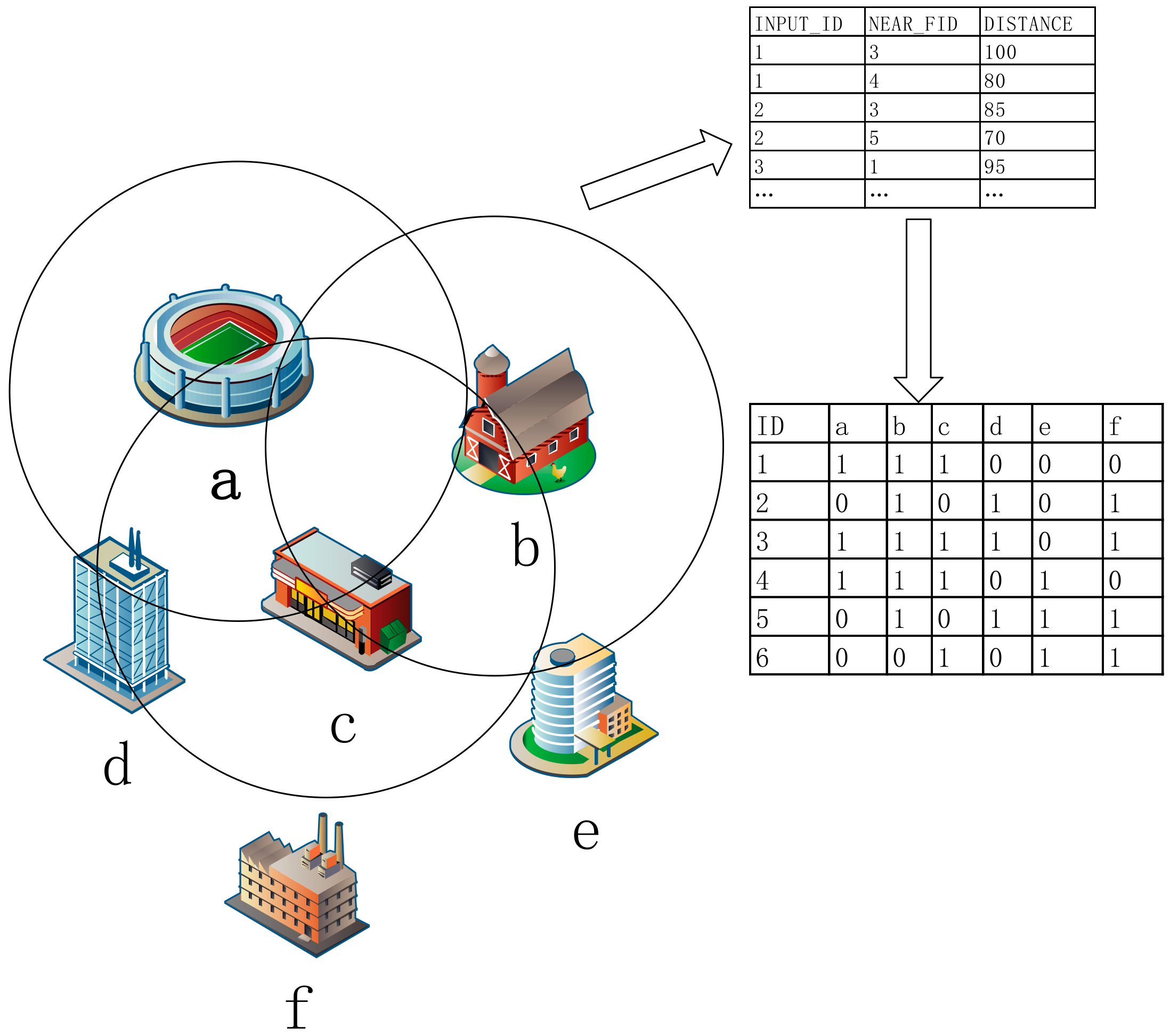
The formal context can correspond to the actual transaction in the urban service industry calculation. An arbitrary spatial location in the city system is an object, and everything around an arbitrary spatial position (such as hospitals, supermarkets, hotels, etc.) is an attribute; then, all spatial points in a city can be regarded as collections of objects, and all the entity types that appear can be considered as collections of all attributes. Then, $uRa$ can be expressed as whether there are hotels, snack shops and other service shops in the vicinity of a certain location; for example, if there is a distribution of hotels around the railway station without the distribution of fast food restaurants, it can be expressed as $R$ (railway station, hotel) $=1$, $R$(railway station, fast food restaurant) $=0$. The distribution of various entity types can be converted into a formal context problem in a city.

As shown in Figure 1, the service types of each entity are assumed to be $a$ (snack shop), $b$ (apartment hotel), $c$ (beauty salon), $d$ (three-star hotel), $e$ (Chinese restaurant), and $f$ (budget hotel). The spatial distribution of the urban services industry can be converted into a formal context, where $U$ = {1, 2, 3, 4, 5, 6} and $A$ = {$a,b,c,d,e,f$}. The formal context naturally corresponds to the actual transaction in the urban service industry calculation. An arbitrary spatial location in the city system is an object (such as 1), and everything around an arbitrary spatial position (such as $a$, $b$, $c$, etc.) is its attribute. Hence, all spatial points in a city can be regarded as collections of objects, and all of the entity types that appear can be considered as collections of all attributes. Finally, $uRa$ can be expressed as whether there are hotels, snack shops and other service shops in the vicinity of a certain location. The study of the distribution of various entity types can be converted into a formal context analysis problem in a city.

Definition 2

[27].A Galois relationship is a pair of mappings between the set of arbitrary objects $E\subseteq U$ and the set of arbitrary attributes $I\subseteq A$:

$$f\left(E\right)= \{a\in A |\forall u\in E, uRa\}$$

(2)

and

$$g\left(I\right)= \{u\in U |\forall a\in I, uRa\}.$$

(3)

Definition 3

[27].Let $E\subseteq U$ and $I\subseteq A$ if tuple $C=\left(E, I\right)$ meets the following:

$$f\left(E\right)= I \mathrm{and}g\left(I\right) = E.$$

(4)

Then, $C$ is a formal concept for $F$, referred to as the concept. The collection of all concepts on the formal context is recorded as $CS\left(F\right)$.

Definition 4

[11].Let concepts $C_1=\left(E_1, I_1\right)$ and $C_2=\left(E_2, I_2\right)$ meet $E_1\subseteq E_2$ or $I_2\subseteq I_1$. If there is no $\forall C_3=\left(E_3, I_3\right)\in CS\left(F\right)$ can make

$$E_1\subseteq E_3\subseteq E_2 \mathrm{or} I_2\subseteq I_3\subseteq I_1.$$

(5)

We say that there is a partial order relationship between $C_1$ and $C_2$, denoted as $C_1<C_2$ or $C_2>C_1$. We often refer to $C_1$ as the sub-concept of $C_2$, and $C_2$ as the parent concept of $C_1$.

Definition 5

[11].The concept lattice is a tuple:

$$L=(CS\left(F\right), <)$$

(6)

Namely, a concept lattice is composed of the entire concept $CS\left(F\right)$ from the formal context $F$ and the partial order relationship $<$ between the two concepts.

The calculation and analysis of the concept lattice problem can be carried out for spatial association and aggregation of the urban service industry. To calculate the distance between the two entities, a given radius (such as a 100-$m$ distance around each entity shop) can be used to calculate all business services within the distance between adjacent points in actual computation, and then the distance table can be created using a specific search radius within the scope of the distance between the two groups of points. The distance table is a property table that is based on a spatial point adjacent to a distance threshold.

2.2. Frequent Closed Itemset

Through the transformation of the formal context, the transaction was replaced by the spatial neighborhoods in the transaction database. The spatial association rule is converted into the spatial co-location rule so that the spatial association problem can be generalized as the point collection database of the spatial index. Therefore, it is possible to find the co-location subsets of frequent spatial event types according to the location map to find the spatial co-location pattern, while the co-location subset corresponds to the itemset in the transaction database. The distance threshold of 100 meters is set in Figure 1, and $a, b,$ and $c$ are in the vicinity of point 1, so {$a,b,c$} is the spatial neighborhood of point 1, which is the transaction in the spatial database.

The definitions are presented as follows.

Definition 6

[28].Given the formal context $F=\left(U, A, R\right)$, the support of any concept $C=\left(E,I\right)$ is

$$Sup\left(C\right)=\frac{\left|E\right|}{\left|U\right|}$$

(7)

Definition 7

[28].Given frequent threshold $\rho$, concept $C=\left(E,I\right)$ is called frequent if and only if

$$Sup\left(C\right)\ge \rho .$$

(8)

$\left\{a\right\},\left\{b\right\},\mathrm{and}\left\{c\right\}$ are 1-itemsets and $\left\{a,b\right\},\left\{b,c\right\}$ are 2-itemsets in Figure 1. If the minimum support degree is set to 30%, the 2-itemset $\left\{a,b\right\}$ appears three times, but the formal context has six objects, so the support degree is 50% greater than the minimum support degree; thus, the 2-itemset $\left\{a,b\right\}$ can be called a frequent itemset. The spatial partition has generally been used in previous methods to produce a series of transactions in the spatial database, resulting in a different set of items, through the iterative method of layer-by-layer search, scanning the itemset of each item to facilitate using an Apriori algorithm. The algorithm of the scanning itemset can get six 1-itemsets, 15 2-itemsets, 20 3-itemsets, 15 4-itemsets, and six 5-itemsets, for a total of 62 itemsets in Figure 1. If the minimum support degree is set to 0.3, then it can get 18 frequent itemsets in Figure 1.

The relation of the concept lattice is two mappings between the object sets and the attribute sets, which can be defined as a closed operation $\mathsf{\gamma }=\mathsf{\alpha }\cdot \mathsf{\beta }=\mathsf{\beta }\left(\mathsf{\alpha }\left(\mathrm{l}\right)\right)$; for itemset $\mathrm{l}$, the closed operation $\mathsf{\gamma }\left(\mathrm{l}\right)$ represents the largest itemset that contains all objects the itemset $\mathrm{l}$ has. For frequent itemset $\mathrm{l}$, if $\mathsf{\gamma }\left(\mathrm{l}\right)=\mathrm{l}$, then the itemset is a closed itemset; if it meets greater than the minimum support degree, then the itemset is a frequent closed itemset. A closed itemset refers to an itemset for which the support count of its direct super set is not equal to its own support count. The occurrence count of itemset $\left\{\mathrm{e},\mathrm{f}\right\}$ is 2, but the occurrence count of the direct super set $\left\{\mathrm{b},\mathrm{d},\mathrm{e},\mathrm{f}\right\}$, $\left\{\mathrm{c},\mathrm{e},\mathrm{f}\right\}$ of itemset $\left\{\mathrm{e},\mathrm{f}\right\}$ is 1, which is not equal to the occurrence count of itemset $\left\{\mathrm{e},\mathrm{f}\right\}$, so the itemset $\left\{\mathrm{e},\mathrm{f}\right\}$ is a closed itemset; if the minimum support degree is set to 30%, the itemset $\left\{\mathrm{e},\mathrm{f}\right\}$ is also a frequent closed itemset. The occurrence count of itemset $\left\{\mathrm{a},\mathrm{b}\right\}$ is 3, but the occurrence count of super item $\left\{\mathrm{a},\mathrm{b},\mathrm{c}\right\}$ for itemset $\left\{\mathrm{a},\mathrm{b}\right\}$ is 3, so the itemset $\left\{\mathrm{a},\mathrm{b}\right\}$ is not a closed itemset.

2.3. Spatial Association Rule

Each concept lattice node is essentially a maximum itemset; it provides a platform for the mining of association rules, which embodies the inclusion and classification of concepts. Because the rule itself is described by the relation between the intent of the concept lattice, while it represents the including and included relations between the extent of the concept lattice, so the concept node unifies the relationship between the intent and extent of the concept lattice. The association rule is generally denoted as $X\to Y$, where the left itemset $X$ is the prerequisite condition, and the right itemset $Y$ is the corresponding association result, which is used to represent the implied association in the data. For example, the association rule {hotel $\to$ cake shop} represents that the two spatial entities of the hotel and cake shop have a certain degree of association and aggregation.

As for the strength of the spatial association, for example, which is the higher degree of aggregation between hotel and cake shop, snack shop or private restaurant? It is expressed by the association analysis of the two core concepts of support degree and confidence degree. For example, there are 10,000 spatial service entities, including 1000 hotels, 2000 cake shops, and 500 private restaurants, and there are 800 hotels spatially associated with cake shops and 100 hotels spatially associated with private restaurants.

Support degree [8]: The probability of the occurrence of all the itemsets $\left\{X, Y\right\}$, that is, the probability of $X$ and $Y$ occurring at the same time.

$$\mathit{S}\mathit{u}\mathit{p}\left(\mathit{X}\to \mathit{Y}\right)=\mathit{S}\mathit{u}\mathit{p}\left(\left\{\mathit{X}, \mathit{Y}\right\}\right)$$

(9)

In general, a minimum threshold (minsup, Minimum Support) is set to eliminate the spatial position association rule with a low appearance ratio to reserve the more frequent rules of closed itemsets. Spatial association rules are generated on the basis of frequent closed itemsets, so the support degree is equal to the frequent closed itemsets. In the above specific spatial service entity data, the minimum threshold is assumed to be 5% due to the support of {hotel, cake shop} being 800/10,000$=$8%, but the support of {hotel, private restaurant} is 100/10,000$=$1%, so the frequent closed itemset {hotel, cake shop} meets the basic support requirements, and it is a spatial closed frequent itemset; then, the spatial association rule hotel $\to$ cake shop and cake shop $\to$ hotel are reserved at the same time, but the two spatial association rules of the spatial itemset {hotel, private restaurant} are eliminated.

Confidence degree [8]. The probability that the associated result $Y$ occurs under the condition of occurrence that the prerequisite condition $X$ of association rule, that is, it is the possibility of $Y$ when it has $X$ in an itemset at the same time.

$$\mathit{Conf}\left(\mathit{X}\to \mathit{Y}\right) = \mathit{p}(\mathit{Y} | \mathit{X}) = \mathit{S}\mathit{u}\mathit{p}\left(\mathit{X}, \mathit{Y}\right)/\mathit{S}\mathit{u}\mathit{p}\left(\mathit{X}\right)$$

(10)

The confidence degree is the second threshold for generating strong association rules, and a minimum threshold ($\mathrm{mincon}$, Minimum Confidence) is required to continue filtering. In the above-mentioned context, when the minimum threshold is 70%, the confidence degree of the rule hotel $\to$ cake shop is 800/1000$=$80%, but the confidence degree of the rule cake shop $\to$ hotel is 800/2000$=$40%; then, the rule hotel $\to$ cake shop is reserved, and the rule cake shop $\to$ hotel is eliminated.

3. Spatial Association Discovery

3.1. Frequent Closed Itemset Discovery

The node of the concept lattice corresponds to the itemset in the association analysis, and the following conclusions can be drawn from the characteristics of frequent closed itemsets and the concept lattice:

(1)

Each node of the concept lattice is a closed itemset, but it is not necessarily a frequent closed itemset.

(2)

All intent sets of the concept lattice are equal to a collection of closed itemsets that can be derived from a spatial transaction database.

(3)

Frequent closed itemsets can filter out redundant information in frequent itemsets. This not only can determine the frequency information of all frequent itemsets, but is also several orders of magnitude smaller than frequent itemsets.

To obtain the concept lattice from the formal context, the following operational definition is needed.

Definition 8

[29].Given a formal context $F=\left(U, A, R\right)$, we can define operations on object sets $X\subseteq U$ and attribute sets $B\subseteq A$ as

$$\left\{\begin{array}{c}{X}^{*}= \{a |a\in A, \forall x\in X, xRa\};\\ B^{*}= \{x |x\in U, \forall a\in B, xRa\}.\end{array}\right.$$

(11)

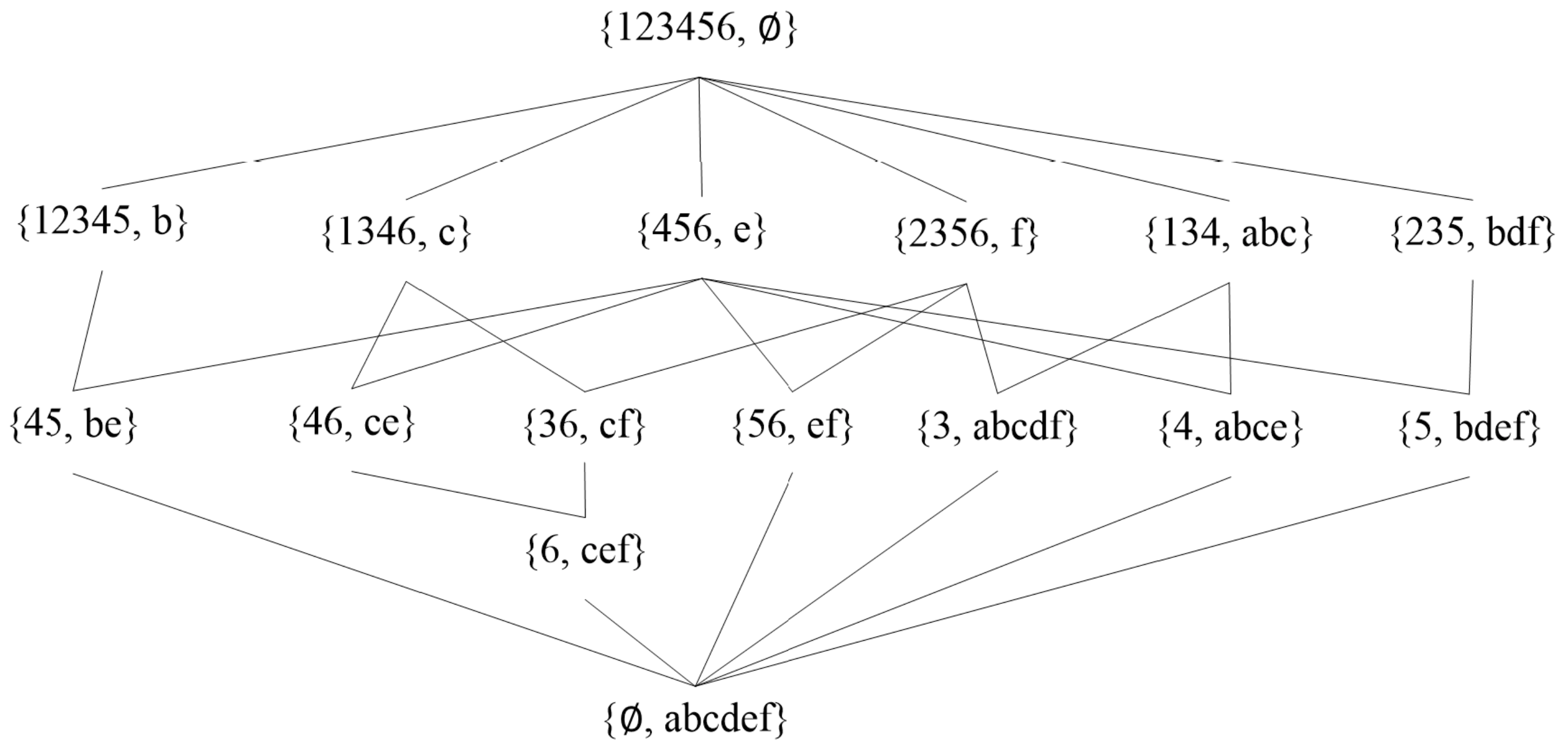
A total of 15 closed itemsets from the above definitions are obtained, the minimum support degree is also set to 0.3, and 10 frequent closed itemsets can be obtained. Along with the increase in the number, frequent closed itemsets are orders of magnitude smaller than frequent itemsets without losing all the frequency information of frequent itemsets and thus can produce spatial association rules. It is listed in detail in Figure 2 and

Table 1. Comparison table of frequent itemsets and frequent closed itemsets for Figure 1.

Frequent Itemsets						Frequent Closed Itemsets
Itemsets	Support	Itemsets	Support	Itemsets	Support	Closed Itemsets	Support	Closed Itemsets	Support
$\mathit{b}$	83	$\mathit{b},\mathit{c}$	50	$\mathit{a},\mathit{c}$	50	$\mathit{b}$	83	$\mathit{b},\mathit{e}$	33
$\mathit{c}$	67	$\mathit{b},\mathit{f}$	50	$\mathit{c},\mathit{e}$	33	$\mathit{c}$	67	$\mathit{c},\mathit{e}$	33
$\mathit{f}$	67	$\mathit{a},\mathit{b}$	50	$\mathit{d},\mathit{f}$	50	$\mathit{e}$	50	$\mathit{c},\mathit{f}$	33
$\mathit{a}$	50	$\mathit{b},\mathit{d}$	$50$	$\mathit{c},\mathit{f}$	33	$\mathit{f}$	67	$\mathit{e},\mathit{f}$	33
$\mathit{d}$	50	$\mathit{b},\mathit{e}$	33	$\mathit{a},\mathit{b},\mathit{c}$	50	$\mathit{a},\mathit{b},\mathit{c}$	50	-	-
$\mathit{f}$	50	$\mathit{c},\mathit{f}$	33	$\mathit{b},\mathit{d},\mathit{f}$	50	$\mathit{b},\mathit{d},\mathit{f}$	83	-	-

.

The frequent closed itemsets discovery algorithms have been designed based on the concept of the concept lattice and frequent closed itemsets, and the detailed algorithms are seen in Algorithm 1 and Algorithm 2. The inputs of Algorithm 1 are included: the given formal context ${\mathrm{F}}^{\mathrm{T}}$ is transposed from $\mathrm{F}$, and frequent threshold value $\mathsf{\rho }$, the outputs are all frequent closed itemsets and the partial order relationship between them, and these partial order relationships are generated by Algorithm 2. Newly added attributes will create new concepts; to guarantee the uniqueness of the new concept, Algorithm 1 introduces two conditions: 1) the extent of all concepts except concept $\mathrm{C}$ are not equal to $ℂ$; and 2) the intersection of all the extents of parent concepts and $\mathrm{E}\left(\left\{\mathrm{a}\right\}\right)$ is not equal to $ℂ$. When the two conditions are met simultaneously, the algorithm will produce a new frequent concept ${\mathrm{C}}^{*}=\left(\mathrm{C}\left(\mathrm{I}\right)\cup \left\{\mathrm{a}\right\},ℂ\right)$.

Algorithm 1.	Frequent Closed Itemsets Lattice Discovery.
Input:	Formal context $F^T=\left(A,U,R^T\right)$, frequent threshold $\rho$;
Output:	Frequent closed itemsets lattice $FL=\left(FCS\left(F\right),\le ,\rho \right)$;
1.	Let $FCS=\left\{\left(A,\varphi \right),\left(\varphi ,U\right)\right\}$;
2.	FOR (each $a\in A$ and $\frac{\left|E\left(\left\{a\right\}\right)\right|}{\left|U\right|}\ge \rho$) DO
3.	FOR (each concept $C\in FCS$) DO
4.	Let $ℂ=E\left(\left\{a\right\}\right)\cap C\left(E\right)$ s.t. $\frac{\left|ℂ\right|}{\left|U\right|}\ge \rho$;
5.	Let $C\left(I\right)=C\left(I\right) \cup \left\{a\right\}$ when $\left|ℂ\right|\mathrm{equals}\left|C\left(E\right)\right|$;
6.	IF(there is no $C’\in FCS$ s.t. $ℂ==C’\left(E\right)$) THEN
7.	IF(there is no $C^{″}>C$ s.t. $ℂ==C^{″}\left(E\right)\cap E\left(\left\{a\right\}\right)$) THEN
8.	Generate concept $C^{*}=\left(C\left(I\right) \cup \left\{a\right\},ℂ\right)$;
9.	Let $FCS=FCS\cup \left\{C^{*}\right\}$;
10.	Update-$FL\left(C^{*}\right)$; //Update the $"\le "$ relationship.
11.	ENDIF
12.	ENDIF
13.	ENDFOR
14.	ENDFOR

Algorithm 2.	Update the $"\le "$ Relationship of a New Concept.
Input:	New concept $C^{*}$;
Output:	New FL;
Method:	Update-$FL$;
1.	// Step 1. Add all candidate parents and children relationships.
2.	FOR (each concept $C\in FCS$) DO
3.	IF($C^{*}\left(E\right)\subseteq C\left(E\right)$) THEN
4.	$C$.children =$C$.children $\cup \left\{C^{*}\right\}$ and $C^{*}$.parent =$C^{*}$.parent $\cup \left\{C\right\}$;
5.	ELSE IF($C\left(E\right)\subseteq C^{*}\left(E\right)$)
6.	$C$.parent =$C$.parent $\cup \left\{C^{*}\right\}$ and $C^{*}$.children =$C^{*}$.children $\cup \left\{C\right\}$;
7.	ENDIF
8.	ENDFOR
9.	// Step 2. Remove redundant parents and children relationships.
10.	FOR(each concept $C\in C^{*}$.parent and $C^{\prime }\in C^{*}$.parent) DO
11.	Remove the edge/relationship between $C^{*}$ and $C^{\prime }$ if $C\left(E\right)\subseteq C^{\prime }\left(E\right)$;
12.	ENDFOR
13.	FOR(each concept $C\in C^{*}$.children and $C^{\prime }\in C^{*}$.children) DO
14.	Remove the edge/relationship between $C^{*}$ and $C$ if $C\left(E\right)\subseteq C^{\prime }\left(E\right)$;
15.	ENDFOR
16.	// Step 3. Remove redundant grandpas and grandchildren relationships.
17.	FOR(each concept $C\in C^{*}$.parent and $C^{\prime }\in C^{*}$.children) DO
18.	Remove the edge/relationship between $C^{\prime }$ and $C$ if $C^{\prime }\in C$.children or $C\in C^{\prime }$.parent;
19.	ENDFOR

3.2. Spatial Association Rule Discovery

Once the spatial frequent closed itemsets are mined, spatial association rules can be directly generated by these itemsets that are greater than the minimum support degree and minimum confidence degree; the specific production process is as follows:

• For each frequent closed itemset, all of the non-empty subsets $l$ are generated;
• For each non-empty subset $s$ of $l$, if $\mathrm{Conf}$ $\left(s\to l-s\right)\ge \mathrm{mincon}$, then $s\to l-s$ is exported.

The minimum support degree is 50% and the minimum confidence degree is 75% in Figure 1, and then all association rules from frequent closed itemsets can be obtained in

Table 2. Spatial association rules from frequent closed itemsets.

Rules	Support	Confidence	Rules	Support	Confidence
$\mathit{a}\to \mathit{b}$	50%	100%	$\mathit{b}\mathit{c}\to \mathit{a}$	50%	100%
$\mathit{a}\to \mathit{c}$	50%	100%	$\mathit{e}\to \mathit{b}$	33.3%	100%
$\mathit{a}\to \mathit{b}\mathit{c}$	50%	100%	$\mathit{f}\to \mathit{b}$	50%	75%
$\mathit{c}\to \mathit{a}$	50%	75%	$\mathit{f}\to \mathit{d}$	50%	75%
$\mathit{c}\to \mathit{b}$	50%	75%	$\mathit{f}\to \mathit{b}\mathit{d}$	50%	75%
$\mathit{c}\to \mathit{a}\mathit{b}$	50%	75%	$\mathit{b}\mathit{d}\to \mathit{f}$	50%	100%
$\mathit{a}\mathit{b}\to \mathit{c}$	50%	100%	$\mathit{b}\mathit{f}\to \mathit{d}$	50%	100%
$\mathit{a}\mathit{c}\to \mathit{b}$	50%	100%	$\mathit{d}\mathit{f}\to \mathit{b}$	50%	100%

. It can be seen that there are fewer redundant rules than frequent itemsets. For example, the frequent itemset $\left\{a,b\right\}$ is not a frequent closed itemset, but it appears in nodes $\left\{a,b\right\}$ and $\left\{a,b,c\right\}$, so the rule $a\to b$ will be produced by these nodes at the same time, and there are redundant rules that will increase the computational burden.

The algorithms to derive all of the spatial association rules have also been designed based on the spatial frequent closed itemset $FL$, and the detailed processes are seen in Algorithm 3 and Algorithm 4.

Algorithm 3.	Generate Association Rules.
Input:	$\mathit{F}\mathit{L}=\left(\mathbf{F}\mathbf{C}\mathbf{S}\left(\mathbf{F}\right),\le ,\mathit{\rho }\right)$, confidence threshold $\mathit{\delta }$;
Output:	The set of association rules $\mathit{𝕽}=\left\{\mathbf{r}\right|\mathbf{C}\mathbf{o}\mathbf{n}\mathbf{f}\left(\mathbf{r}\right)\ge \mathit{\delta }\}$;
Method:	GAR;
1.	Initialize $\mathit{𝕽}=\left\{\right\}$; // The set of association rules.
2.	FOR (each concept $\mathit{C}\in \mathit{F}\mathit{L}$ and $\left|\mathit{C}\right|\ge \mathit{2}$) DO
3.	${\mathit{H}}_{\mathit{1}}=\left\{\left\{{\mathit{h}}_{\mathit{1}}\right\}\right|{\mathit{h}}_{\mathit{1}}\in \mathit{C}\left(\mathit{I}\right)\}$
4.	FOR (each $\left\{{\mathit{h}}_{\mathit{1}}\right\}\in {\mathit{H}}_{\mathit{1}}$) DO
5.	$\mathbf{C}\mathbf{o}\mathbf{n}\mathbf{f}$ = $\frac{\mathbf{S}\mathbf{u}\mathbf{p}\left(\mathit{C}\right)}{\mathbf{S}\mathbf{u}\mathbf{p}\left(\mathit{C}-\left\{{\mathit{h}}_{\mathit{1}}\right\}\right)}$;
6.	IF ($\mathbf{C}\mathbf{o}\mathbf{n}\mathbf{f} \ge \mathit{\delta }$) THEN
7.	$\mathit{𝕽}=\mathit{𝕽}\cup \left\{\mathit{r}:\left\{\mathit{C}-\left\{{\mathit{h}}_{\mathit{1}}\right\}\right\}\Rightarrow \left\{{\mathit{h}}_{\mathit{1}}\right\}\right\}$;
8.	ELSE
9.	${\mathit{H}}_{\mathit{1}}={\mathit{H}}_{\mathit{1}}-\left\{{\mathit{h}}_{\mathit{1}}\right\}$;
10.	ENDIF
11.	ENDFOR
12.	Longer-Rules($\mathit{C}, {\mathit{H}}_{\mathit{1}}$);
13.	ENDFOR

The inputs include the frequent closed itemsets $FL$ and confidence threshold value $\delta$ in Algorithm 3, and a rule is confident when and only if its confidence degree is not less than $\delta$. The basic idea of the algorithm also consists of two steps, namely, it generates a confident rule with a "result" length of 1 and then generates the other rules with longer "result" lengths. First, “result” is denoted as the latter part of an association rule. Hence, they are actually the subset of an itemset. Second, the length of “result” is one means by which the corresponding itemset (i.e., the latter part of an association rule) only contains one item. Third, because the purpose of our work is to obtain the entire set of confident association rules, the size of the resulted itemset should be increased. This process is implemented by Line 2 in Algorithm 4. In detail, given two itemsets with length m-1, their previous m-2 items being the same, and their last items being different, the two itemsets can be merged into one new itemset with length k. For example, {a, b, c} and {a, b, d} can be merged into {a, b, c, d} (m = 4). For each of the frequent closed itemsets (concepts) in $FL$, there is a recursive procedure, that is, the next itemset is processed after all of the confident rules are derived from the current itemset. There is a condition $\left|\mathrm{C}\right|\ge 2$ in line 2 of Algorithm 3 because the rule cannot be generated when the number of attributes is 1.

Algorithm 4.	Generate Association Rules with Longer Result.
Input:	Concept $\mathit{C}, {\mathit{H}}_{\mathit{m}}$ the set of subset with length $\mathit{m}$;
Method:	Longer-Rules;
1.	IF($\left|\mathit{C}\left(\mathit{I}\right)\right|>\mathit{m}+\mathit{1}$) THEN
2.	${\mathit{H}}_{\mathit{m}+\mathit{1}}=$ Growth(${\mathit{H}}_{\mathit{m}}$);
3.	FOR (each ${\mathit{h}}_{\mathit{m}+\mathit{1}}\in {\mathit{H}}_{\mathit{m}+\mathit{1}}$) DO
4.	$\mathbf{C}\mathbf{o}\mathbf{n}\mathbf{f}$ = $\frac{\mathbf{S}\mathbf{u}\mathbf{p}\left(\mathit{C}\right)}{\mathbf{S}\mathbf{u}\mathbf{p}\left(\mathit{C}-\left\{{\mathit{h}}_{\mathit{m}+\mathit{1}}\right\}\right)}$
5.	IF ($\mathbf{C}\mathbf{o}\mathbf{n}\mathbf{f} \ge \mathit{\delta }$) THEN
6.	$\mathit{𝕽}=\mathit{𝕽}\cup \left\{\mathit{r}:\left\{\mathit{C}-\left\{{\mathit{h}}_{\mathit{m}+\mathit{1}}\right\}\right\}\Rightarrow \left\{{\mathit{h}}_{\mathit{m}+\mathit{1}}\right\}\right\}$;
7.	ELSE
8.	${\mathit{H}}_{\mathit{m}+\mathit{1}}={\mathit{H}}_{\mathit{m}+\mathit{1}}-\left\{{\mathit{h}}_{\mathit{m}+\mathit{1}}\right\}$;
9.	ENDIF
10.	Call Generate-Rules($\mathit{C}, {\mathit{H}}_{\mathit{1}}$);
11.	ENDFOR
12.	ENDIF

4. Case Study

4.1. Research Area and Data Sources

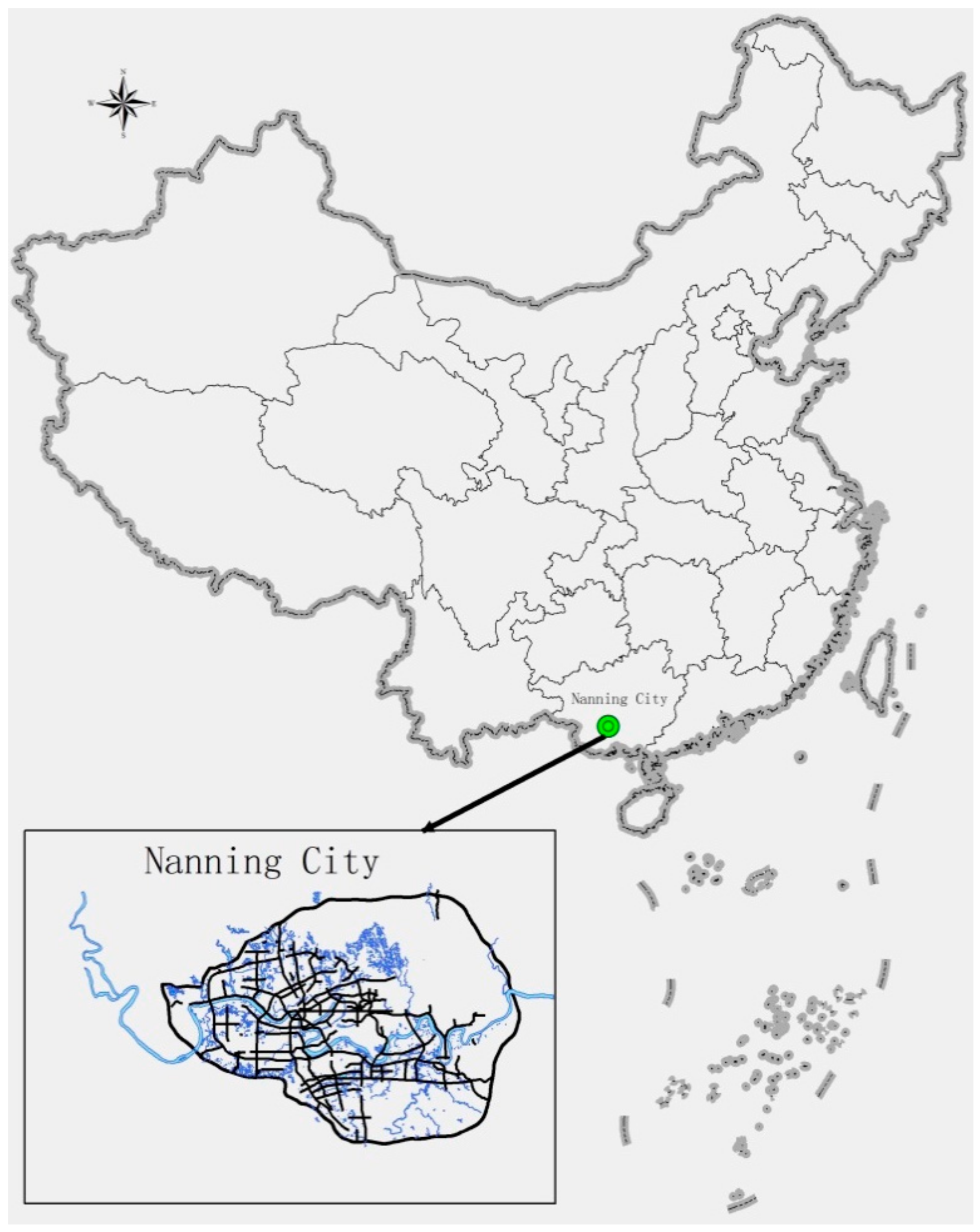
To verify the practicability of this approach, this paper studies the association and aggregation of the urban service industry in Nanning city, China. Nanning is the capital of the Guangxi Zhuang Autonomous Region of China, the specific location is seen in Figure 3. The urban service industry of Nanning is very developed. A total of five categories, 88 small departments (https://nn.nuomi.com), and more than 13,000 information records with coordinates were obtained. On this basis, those with a number of records fewer than 10 were excluded, and a total of 68 departments and 12,739 spatial service entities were obtained.

4.2. Computing Framework

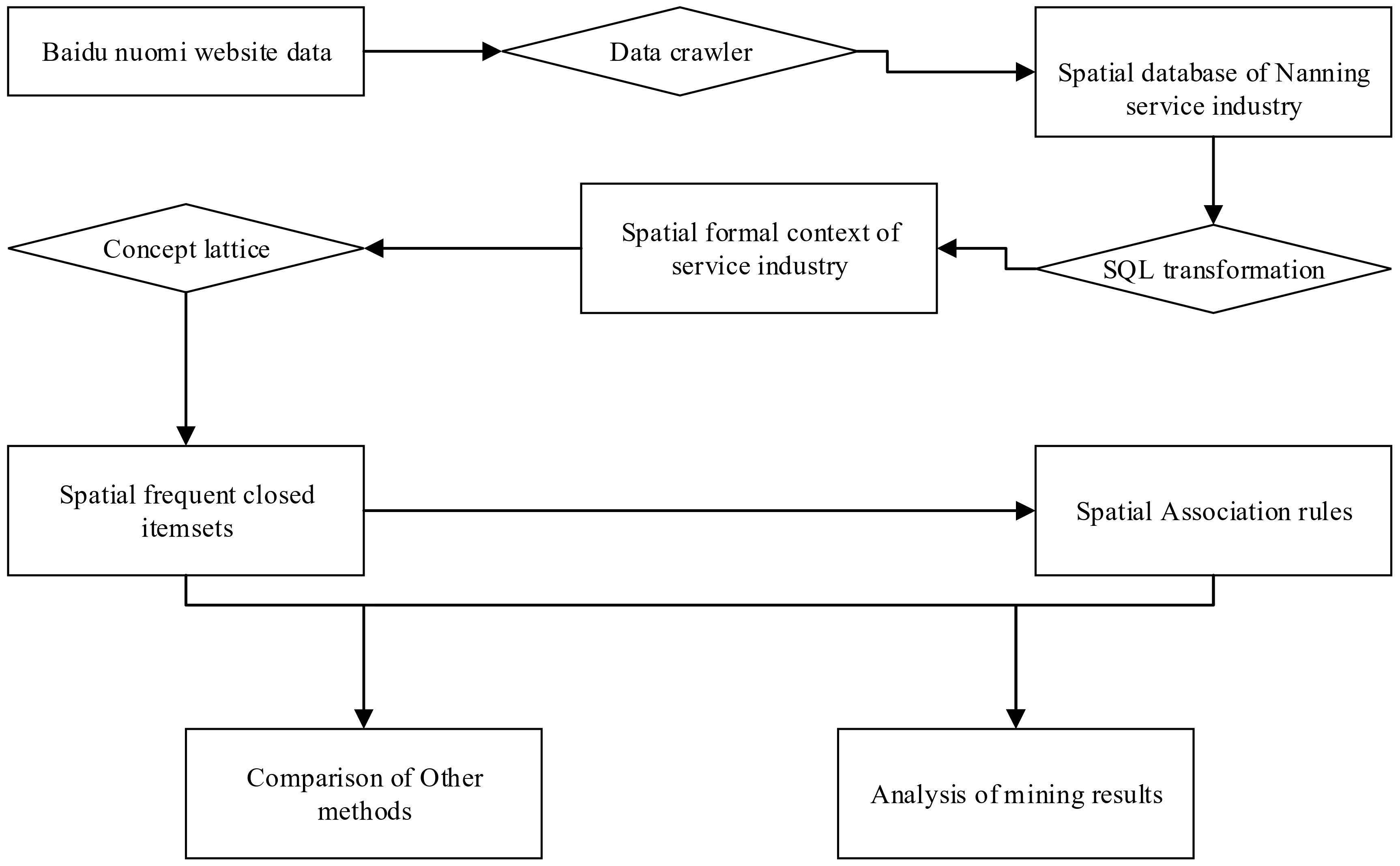
This study used Python crawler technology to obtain real-time spatial data of the urban service industry from the Baidu Nuomi website and established a spatial database of the Nanning service industry, including spatial location. In the ARC GIS platform, the spatial data of the urban service industry in the case area were converted into a neighborhood table by the near operation based on the linear distance neighborhood. To mine and calculate the concept lattice, we used SQL technology to transform the spatial neighborhood table of the service industry into the spatial formal context of the service industry composed of 0 and 1. Using Algorithms 1 and 2, the spatial association concept and frequent closed itemsets of the Nanning service industry were mined on the basis of spatial formal context. The spatial association rules of the urban service industry were mined by Algorithms 3 and 4 on the basis of frequent closed itemsets. According to the frequent closed itemsets and spatial association rules of the service industry, we analyzed the spatial association characteristics of the service industry in Nanning and compared superiority and applicability with other mining methods. The specific process is seen in Figure 4.

4.3. Results Analysis

Four distance thresholds of 10 meters, 50 meters, 100 meters, and 200 meters were tested. Due to space reasons, the following only discusses the case of the distance threshold of 100 meters. The minimum support degree for designing frequent closed itemsets was 0.1 in this study. The following Table 3 lists the top 20 frequent 2-frequent closed itemsets and frequent 3-frequent closed itemsets arranged in descending order of support.

The snack food appears in many frequent closed itemsets with high ordering, as can be seen from Table 3, and the frequency is also very high in other distance thresholds. This shows that snack food is a type of popular consumption entity store, which is distributed around various industries. The snack food industry in Nanning does not have the characteristics of being aggregated with other industries. However, through the distance threshold analysis of 10 meters, 50 meters, and 100 meters, the popular consumption hotels in Nanning have the characteristic of compact layout, which shows that the practitioners of the popular consumption type of hotel industry in Nanning are interested in the layout of the competitors, thus improving the passenger flow and forming the spatial aggregation of the regional industry brand. Similarly, many cognitive rules can be summed up; for example, we can see that the support degree of the 2-frequent closed itemset is higher than that of the 3-frequent closed itemset in the results because the probability of 2 types of industries in one place is greater than the probability of having 3 types of industries, which is also in line with our cognition.

The top 30 spatial association rules based on frequent closed itemsets in Nanning are listed in the following

Table 4. Top 20 confident association rules from Table 3.

Rules	Support	Confidence Degree
{Sweet Drinks}$\to${Snack Food}	0.470	0.901
{Snack Food}$\to${Sweet Drinks}	0.470	0.647
{Beauty}$\to${Snack Food}	0.445	0.828
{Snack Food}$\to${Beauty}	0.445	0.613
{Cake}$\to${Snack Food}	0.409	0.863
{Other Foods}$\to${Snack Food}	0.401	0.900
{Sweet Drinks}$\to${Beauty}	0.359	0.688
{Beauty}$\to${Sweet Drinks}	0.359	0.668
{Cake}$\to${Sweet Drinks}	0.350	0.739
{Sweet Drinks}$\to${Cake}	0.350	0.672
{All Chinese Food}$\to${Snack Food}	0.342	0.886
{Cake}$\to${Beauty}	0.339	0.716
{Beauty}$\to${Cake}	0.339	0.631
{Beauty, Sweet Drinks}$\to${Snack Food}	0.336	0.937
{Sweet Drinks, Snack Food}$\to${Beauty}	0.336	0.716
{Beauty, Snack Food}$\to${Sweet Drinks}	0.336	0.756
{Other Foods}$\to${Sweet Drinks}	0.327	0.733
{Sweet Drinks}$\to${Other Foods}	0.327	0.627
{Cake, Sweet Drinks}$\to${Snack Food}	0.325	0.929
{Cake, Snack Food}$\to${Sweet Drinks}	0.325	0.796

. The snack food appears in the left-hand items and right-hand items of the many rules with high support degrees, which can also be seen in Table 4, and from the other side, the snack food industry in Nanning does not have obvious spatial aggregation with a specific industry. However, for the hotel industry, it is obvious that there are two rules: {General Hotel} $\to$ {Budget Hotel} and {General Hotel} $\to$ {Budget Hotel}. The support is 0.306, and the confidence degrees are 1 and 0.764, respectively, which illustrates the compact layout of the popular consumption type hotel industry in Nanning.

5. Discussions

5.1. Methods of Evaluation

We can find the spatial association of the urban service industry using a quantitative method. Spatial association research is on the basis of frequent itemsets in the past. The frequent itemsets algorithm represented by the Apriori algorithm has already had mature computing packages in the mainstream computing languages and has many commercial applications, which proved the strong application requirement of the association problem. However, these algorithms are not designed to solve spatial problems, and each association rule-mining algorithm has its own application scope. For the mining process based on frequent itemsets, due to the number of scanning instances, the length of itemsets in the R language calculation package must be specified before it can be calculated.

The concept of frequent closed itemsets based on the concept lattice is proposed, and the concept lattice is used as the basic data structure of formal concept analysis. Each concept lattice node can be treated as a closed itemset. With the increase of the number, the frequent closed itemsets are more frequent than the frequent itemsets. The frequent closed itemsets are orders of magnitude smaller but do not lose the frequency information of all frequent itemsets, and they can also generate spatial association rules.

Four distance thresholds of 10 meters, 50 meters, 100 meters, and 200 meters were tested in the case area, and the results of various distance thresholds are similar to those of the Arules package based on the Apriori algorithm in the R language. Both the itemsets and closed itemsets based on the concept lattice are huge, and it is not necessary to calculate all closed itemsets. We carried out the calculation of all closed itemsets within six items for the case area and thus compared the results with the Apriori algorithm. The minimum support degree for designing frequent itemsets and frequent closed itemsets is 0.1, and the Apriori algorithm generates 4111 frequent itemsets, including 291 2-frequent itemsets and 882 3-frequent itemsets. This method generates 3660 frequent closed itemsets, including 264 2-frequent closed itemsets and 789 3-frequent closed itemsets. The support degree value and the order of the frequent closed itemsets in order of support of this method were consistent with the Apriori algorithm in the case study, and this method has a slight advantage over the operation time cost of the length of the specified itemsets. The spatial association rules that are generated by frequent itemsets and frequent closed itemsets are the same. The time spent on rule generation will be small only because the number of closed itemsets is reduced. The lattice miner software (https://sourceforge.net/projects/lattice-miner/) can calculate all closed itemsets, but the computation time was two weeks for the 100 meters threshold, and the rules cannot be customized. The computation time of this method is one week for all closed itemsets.

5.2. Spatial Association Discovery

Through the research of this paper, we found that the physical stores of the service industry were scattered in every corner of the city, and there was a certain spatial association between them in the spatial distribution. Through the association analysis, we can find a spatial aggregation and association between service industries. Spatial association discovery can play an important role in service industry layout, location, and location-based service store recommendation. The spatial association support degree of the service industry will decrease with the increase of the distance threshold. In the city service industry of Nanning, the hotel industry has the characteristic of a compact layout, which shows that all types of mass consumption hotels gather together to form the brand spatial aggregation effect. In different distance thresholds, as a type of mass consumption entity store, snack shops are distributed around various industries, with no clustering characteristics with other industries.

5.3. Limitations and Recommendations for Future Research

The data source in the study was the open information of the Baidu Nuomi website, which could have real-time massive data. Because the user registration was the business itself, not a qualified surveying and mapping company, the spatial coordinate accuracy of the data source was not necessarily guaranteed. Although the data of the study crawled all of the data of the case area in the website, it did not include all of the types of urban service industry and could not summarize all of the associations of the service industry in the case area. In this study, only the software and algorithm of frequent closed itemsets and association rules were implemented, and the transformation of spatial formal text was not implemented in the software.

In terms of future research needs, the software cannot achieve the generation of the association rules of the specified left-hand side item or right-hand side item, and the concise solution of the association rules based on reduction and the visual expression of the results of the itemset and association rules will be our next step.

6. Conclusions

In this paper, the authors proposed a spatial association framework for the urban service industry based on the concept lattice. The process of spatial data mining could be understood as the process of forming concepts and producing knowledge from spatial databases through the learning of large amounts of data. Based on the concept of frequent closed itemsets and the concept lattice, an incremental algorithm for spatial frequent closed sets and a spatial association rule algorithm were designed based on frequent closed itemsets. Finally, the algorithm was implemented, and the software was created. The algorithm and software verification was carried out on the problem of spatial association and aggregation of the urban service industry in Nanning, Guangxi, China. The method proposed in this paper was the extension of the concept lattice in spatial computing and urban computing. It could enrich the application scope of the concept lattice and could also consolidate the mathematical foundation of spatial computing, which was an exploration of the geospatial computing methodology.

References

- Akın, D.; Dökmeci, V. Cluster analysis of interregional migration in Turkey. J. Urban Plan. Dev. 2014, 141, 05014016. [Google Scholar] [CrossRef]
- Croitoru, A.; Wayant, N.; Crooks, A.; Radzikowski, J.; Stefanidis, A. Linking cyber and physical spaces through community detection and clustering in social media feeds. Comput. Environ. Urban Syst. 2015, 53, 47–64. [Google Scholar] [CrossRef]
- Lin, J.; Cromley, R.G. Evaluating geo-located Twitter data as a control layer for areal interpolation of population. Appl. Geogr. 2015, 58, 41–47. [Google Scholar] [CrossRef]
- Shelton, T.; Poorthuis, A.; Graham, M.; Zook, M. Mapping the data shadows of Hurricane Sandy: Uncovering the sociospatial dimensions of ‘big data’. Geoforum 2014, 52, 167–179. [Google Scholar] [CrossRef]
- Zheng, Y.; Capra, L.; Wolfson, O.; Yang, H. Urban computing: Concepts, methodologies, and applications. ACM Trans. Intell. Syst. Technol. (TIST) 2014, 5, 38–55. [Google Scholar] [CrossRef]
- Zheng, Y. Methodologies for Cross-Domain Data Fusion: An Overview. IEEE Trans. Big Data 2015, 1, 16–34. [Google Scholar] [CrossRef]
- Athey, S. Beyond prediction: Using big data for policy problems. Science 2017, 355, 483–485. [Google Scholar] [CrossRef] [Green Version]
- Agrawal, R.; Imieliński, T.; Swami, A. Mining association rules between sets of items in large databases. Proc. SIGMOD 1993, 22, 207–216. [Google Scholar] [CrossRef]
- Yu, W. Identifying and Analyzing the Prevalent Regions of a Co-Location Pattern Using Polygons Clustering Approach. ISPRS Int. J. Geo-Inf. 2017, 6, 259. [Google Scholar] [CrossRef] [Green Version]
- Zhang, B.; Lin, J.C.-W.; Shao, Y.; Fournier-Viger, P.; Djenouri, Y. Maintenance of Discovered High Average-Utility Itemsets in Dynamic Databases. Appl. Sci. 2018, 8, 769. [Google Scholar] [CrossRef] [Green Version]
- Wille, R. Restructuring lattice theory: An approach based on hierarchies of concepts. In Ordered Sets; Springer: Dordrecht, The Netherlands, 1982; pp. 445–470. [Google Scholar]
- Yen, S.J.; Lee, Y.S.; Wang, C.K. An efficient algorithm for incrementally mining frequent closed itemsets. Appl. Intell. 2014, 40, 649–668. [Google Scholar] [CrossRef]
- Kao, L.J.; Huang, Y.P.; Sandnes, F.E. Associating absent frequent itemsets with infrequent items to identify abnormal transactions. Appl. Intell. 2015, 42, 694–706. [Google Scholar] [CrossRef]
- Hamrouni, T.; Yahia, S.B.; Nguifo, E.M. Looking for a structural characterization of the sparseness measure of (frequent closed) itemset contexts. Inf. Sci. 2013, 222, 343–361. [Google Scholar] [CrossRef]
- Wang, J.; Han, J.; Pei, J. Closet+: Searching for the best strategies for mining frequent closed itemsets. In Proceedings of the Ninth ACM SIGKDD International Conference on Knowledge Discovery and Data Mining, Washington, DC, USA, August 2003; pp. 236–245. [Google Scholar]
- Grahne, G.; Zhu, J. Fast algorithms for frequent itemset mining using fp-trees. IEEE Trans. Knowl. Data Eng. 2005, 17, 1347–1362. [Google Scholar] [CrossRef]
- Zou, C.; Zhang, D.; Wan, J.; Hassan, M.M.; Lloret, J. Using concept lattice for personalized recommendation system design. IEEE Syst. J. 2017, 11, 305–314. [Google Scholar] [CrossRef]
- Kuo, R.; Hsu, C.K.; Chang, M.; Heh, J.S. A personalized webpage reconstructor based on concept lattice and association rules. J. Internet Technol. 2011, 12, 1015–1024. [Google Scholar]
- Kim, J.; Chung, H.J.; Jung, Y.; Kim, K.K.; Kim, J.H. BioLattice: A framework for the biological interpretation of microarray gene expression data using concept lattice analysis. J. Biomed. Inform. 2008, 41, 232–241. [Google Scholar] [CrossRef] [Green Version]
- Li, J.; He, Z.; Zhu, Q. An entropy-based weighted concept lattice for merging multi-source geo-ontologies. Entropy 2013, 15, 2303–2318. [Google Scholar] [CrossRef]
- Xie, J.; Yang, M.; Li, J.; Zheng, Z. Rule acquisition and optimal scale selection in multi-scale formal decision contexts and their applications to smart city. Future Gener. Comput. Syst. 2018, 83, 564–581. [Google Scholar] [CrossRef]
- Liao, W.; Hou, D.; Jiang, W. An Approach for a Spatial Data Attribute Similarity Measure Based on Granular Computing Closeness. Appl. Sci. 2019, 9, 2628. [Google Scholar] [CrossRef] [Green Version]
- Sikder, I. A variable precision rough set approach to knowledge discovery in land cover classification. Int. J. Digit. Earth 2016, 9, 1206–1223. [Google Scholar] [CrossRef]
- Zheng, D.; Li, C. Research on Spatial Pattern and Its Industrial Distribution of Commercial Space in Mianyang Based on POI Data. J. Data Anal. Inf. Process. 2020, 8, 20–40. [Google Scholar] [CrossRef] [Green Version]
- Yu, B.; Wang, Z.; Mu, H.; Sun, L.; Hu, F. Identification of Urban Functional Regions Based on Floating Car Track Data and POI Data. Sustainability 2019, 11, 6541. [Google Scholar] [CrossRef] [Green Version]
- Ganter, B.; Wille, R. Formal Concept Analysis: Mathematical Foundations; Springer: Berlin/Heidelberg, Germany, 1999. [Google Scholar]
- Tate, J. Relations between K 2 and Galois cohomology. Invent. Math. 1976, 36, 257–274. [Google Scholar] [CrossRef]
- Min, F.; Wu, Y.; Wu, X. The Apriori property of sequence pattern mining with wildcard gaps. In Proceedings of the 2010 IEEE International Conference on Bioinformatics and Biomedicine Workshops (BIBMW), Hong Kong, China, 18 December 2010; pp. 138–143. [Google Scholar]
- Li, J.; Mei, C.; Wang, J.; Zhang, X. Rule-preserved object compression in formal decision contexts using concept lattices. Knowl. Based Syst. 2014, 71, 435–445. [Google Scholar] [CrossRef]
Figure 1.
Processing diagram for transforming the spatial entity into a formal context.
Figure 2.
Concept lattice for Figure 1.
Figure 3.
Location of Nanning city, China.
Figure 4.
Computing framework for the concept lattice method of spatial association discovery in urban service industry.